A Single-Tree Processing Framework Using Terrestrial Laser Scanning Data for Detecting Forest Regeneration


Abstract
1. Introduction
2. Study Area and Data
2.1. Study Area
2.2. TLS Data
2.3. Reference Data
3. Method
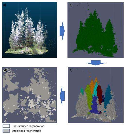
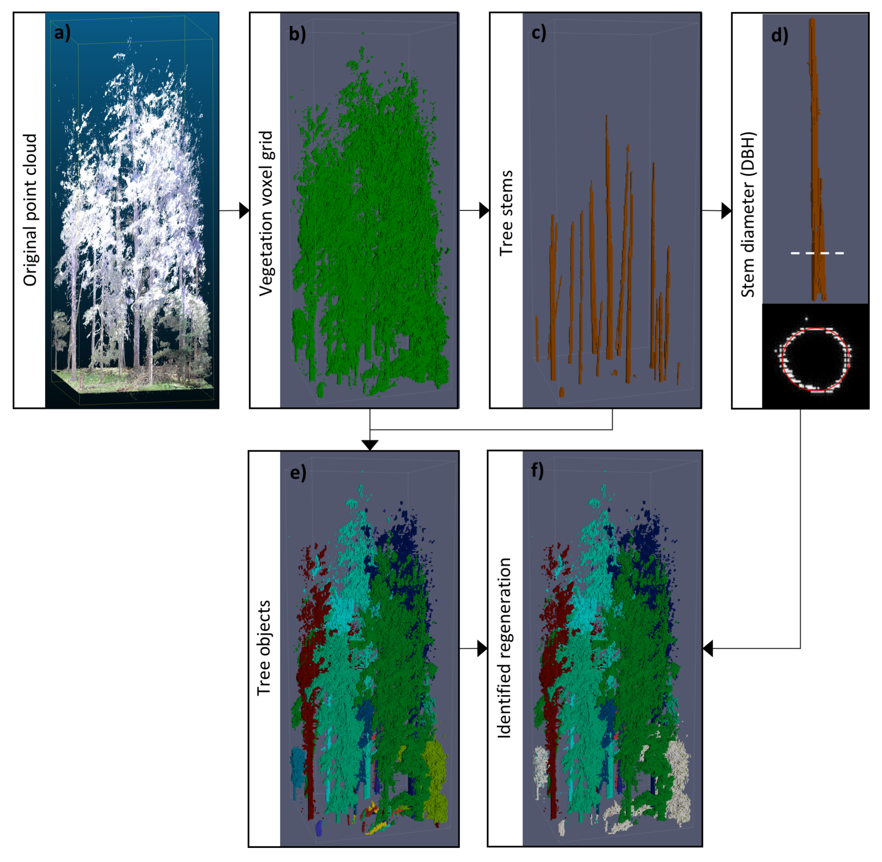
3.1. Outline
3.2. Tree Stem Detection
3.3. DBH Derivation
3.4. Individual Tree Segmentation
3.5. Regeneration Estimation
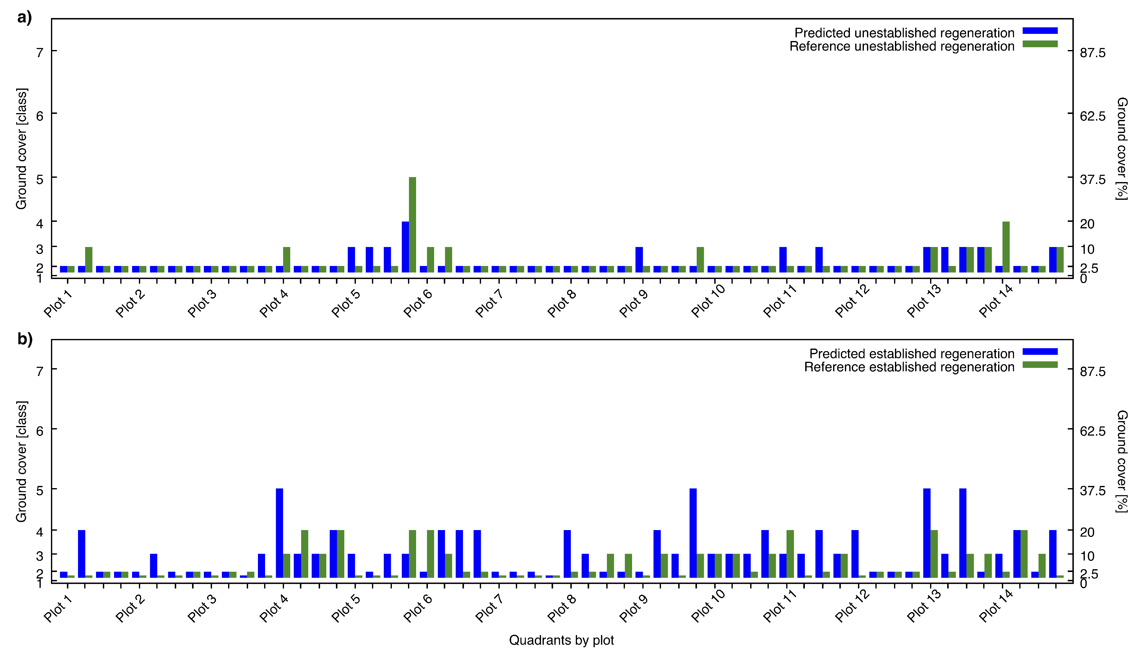
3.6. Accuracy Assessment
4. Results
5. Discussion
5.1. Methodological Approach
5.2. Interpretation of the Results
5.3. Comparison to other Studies
6. Conclusions
Author Contributions
Funding
Acknowledgments
Conflicts of Interest
Abbreviations
| ALS | airborne laser scanning |
| TLS | terrestrial laser scanning |
| MLS | mobile laser scanning |
| LiDAR | light detection and ranging |
| DBH | diameter at breast height |
| CHM | crown height model |
| DSM | digital surface model |
| NFI | national forest inventory |
| SE | structuring element |
| MRF | Markov random field |
| MAE | mean absolute error |
| MBE | mean bias error |
References
- Ishii, H.T.; Tanabe, S.I.; Hiura, T. Exploring the relationships among canopy structure, stand productivity, and biodiversity of temperate forest ecosystems. For. Sci. 2004, 50, 342–355. [Google Scholar]
- Hamraz, H.; Contreras, M.A.; Zhang, J. Vertical stratification of forest canopy for segmentation of understory trees within small-footprint airborne LiDAR point clouds. ISPRS J. Photogramm. Remote Sens. 2017, 130, 385–392. [Google Scholar] [CrossRef]
- Wing, B.M.; Ritchie, M.W.; Boston, K.; Cohen, W.B.; Gitelman, A.; Olsen, M.J. Prediction of understory vegetation cover with airborne lidar in an interior ponderosa pine forest. Remote Sens. Environ. 2012, 124, 730–741. [Google Scholar] [CrossRef]
- O’Hara, K.L. Multiaged forest stands for protection forests: concepts and applications. For. Snow Landsc. Res. 2006, 80, 45–55. [Google Scholar]
- Dorren, L.; Berger, F.; Jonsson, M.; Krautblatter, M.; Mölk, M.; Stoffel, M.; Wehrli, A. State of the art in rockfall—Forest interactions. Schweiz. Z. Forstwes. 2007, 158, 128–141. [Google Scholar] [CrossRef]
- Antos, J. Understory plants in temperate forests. In Forests and Forest Plants; Owens, J.N., Lund, H.G., Eds.; Eolss Publishers Co., Ltd.: Oxford, UK, 2009; pp. 262–279. [Google Scholar]
- Jules, M.J.; Sawyer, J.O.; Jules, E.S. Assessing the relationships between stand development and understory vegetation using a 420-year chronosequence. For. Ecol. Manag. 2008, 255, 2384–2393. [Google Scholar] [CrossRef]
- Latifi, H.; Heurich, M.; Hartig, F.; Müller, J.; Krzystek, P.; Jehl, H.; Dech, S. Estimating over- and understorey canopy density of temperate mixed stands by airborne LiDAR data. Forestry 2015, 89, 69–81. [Google Scholar] [CrossRef]
- Lin, Y.; Holopainen, M.; Kankare, V.; Hyyppa, J. Validation of Mobile Laser Scanning for Understory Tree Characterization in Urban Forest. IEEE J. Sel. Top. Appl. Earth Observ. Remote Sens. 2014, 7, 3167–3173. [Google Scholar] [CrossRef]
- Tuanmu, M.N.; Viña, A.; Bearer, S.; Xu, W.; Ouyang, Z.; Zhang, H.; Liu, J. Mapping understory vegetation using phenological characteristics derived from remotely sensed data. Remote Sens. Environ. 2010, 114, 1833–1844. [Google Scholar] [CrossRef]
- Amiri, N.; Yao, W.; Heurich, M.; Krzystek, P.; Skidmore, A.K. Estimation of regeneration coverage in a temperate forest by 3D segmentation using airborne laser scanning data. Int. J. Appl. Earth Observ. Geoinf. 2016, 52, 252–262. [Google Scholar] [CrossRef]
- Fleming, S.; Cottin, A.; Woodhouse, I. The first spectral map of a forest understory from multispectral lidar. Lidar News 2015, 5, 26–30. [Google Scholar]
- Hill, R.; Broughton, R. Mapping the understorey of deciduous woodland from leaf-on and leaf-off airborne LiDAR data: A case study in lowland Britain. ISPRS J. Photogramm. Remote Sens. 2009, 64, 223–233. [Google Scholar] [CrossRef]
- Korpela, I.; Hovi, A.; Morsdorf, F. Understory trees in airborne LiDAR data—Selective mapping due to transmission losses and echo-triggering mechanisms. Remote Sens. Environ. 2012, 119, 92–104. [Google Scholar] [CrossRef]
- Kükenbrink, D.; Schneider, F.D.; Leiterer, R.; Schaepman, M.E.; Morsdorf, F. Quantification of hidden canopy volume of airborne laser scanning data using a voxel traversal algorithm. Remote Sens. Environ. 2017, 194, 424–436. [Google Scholar] [CrossRef]
- Lindberg, E.; Olofsson, K.; Holmgren, J.; Olsson, H. Estimation of 3D vegetation structure from waveform and discrete return airborne laser scanning data. Remote Sens. Environ. 2012, 118, 151–161. [Google Scholar] [CrossRef]
- Morsdorf, F.; Mårell, A.; Koetz, B.; Cassagne, N.; Pimont, F.; Rigolot, E.; Allgöwer, B. Discrimination of vegetation strata in a multi-layered Mediterranean forest ecosystem using height and intensity information derived from airborne laser scanning. Remote Sens. Environ. 2010, 114, 1403–1415. [Google Scholar] [CrossRef]
- Singh, K.K.; Davis, A.J.; Meentemeyer, R.K. Detecting understory plant invasion in urban forests using LiDAR. Int. J. Appl. Earth Observ. Geoinf. 2015, 38, 267–279. [Google Scholar] [CrossRef]
- Duncanson, L.; Cook, B.; Hurtt, G.; Dubayah, R. An efficient, multi-layered crown delineation algorithm for mapping individual tree structure across multiple ecosystems. Remote Sens. Environ. 2014, 154, 378–386. [Google Scholar] [CrossRef]
- Ferraz, A.; Bretar, F.; Jacquemoud, S.; Gonçalves, G.; Pereira, L.; Tomé, M.; Soares, P. 3-D mapping of a multi-layered Mediterranean forest using ALS data. Remote Sens. Environ. 2012, 121, 210–223. [Google Scholar] [CrossRef]
- Hancock, S.; Anderson, K.; Disney, M.; Gaston, K.J. Measurement of fine-spatial-resolution 3D vegetation structure with airborne waveform lidar: Calibration and validation with voxelised terrestrial lidar. Remote Sens. Environ. 2017, 188, 37–50. [Google Scholar] [CrossRef]
- Gupta, V.; Reinke, K.; Jones, S.; Wallace, L.; Holden, L. Assessing Metrics for Estimating Fire Induced Change in the Forest Understorey Structure Using Terrestrial Laser Scanning. Remote Sens. 2015, 7, 8180–8201. [Google Scholar] [CrossRef]
- Xia, S.; Wang, C.; Pan, F.; Xi, X.; Zeng, H.; Liu, H. Detecting stems in dense and homogeneous forest using single-scan TLS. Forests 2015, 6, 3923–3945. [Google Scholar] [CrossRef]
- Brolly, G.; Király, G.; Czimber, K. Mapping Forest Regeneration from Terrestrial Laser Scans. Acta Silv. Lign. Hung. 2013, 9, 135–146. [Google Scholar] [CrossRef]
- FARO Technologies Inc. FARO Laser Scanner Focus3D Manual; FARO Technologies Inc.: Lake Mary, FL, USA, 2013; p. 79. [Google Scholar]
- Yao, T.; Yang, X.; Zhao, F.; Wang, Z.; Zhang, Q.; Jupp, D.; Lovell, J.; Culvenor, D.; Newnham, G.; Ni-Meister, W.; et al. Measuring forest structure and biomass in New England forest stands using Echidna ground-based lidar. Remote Sens. Environ. 2011, 115, 2965–2974. [Google Scholar] [CrossRef]
- Zande, D.V.d.; Jonckheere, I.; Stuckens, J.; Verstraeten, W.W.; Coppin, P. Sampling design of ground-based lidar measurements of forest canopy structure and its effect on shadowing. Can. J. Remote Sens. 2008, 34, 526–538. [Google Scholar] [CrossRef]
- FARO Technologies Inc. FARO SCENE 5.1 Users Manual; FARO: Lake Mary, FL, USA, 2014. [Google Scholar]
- Bienert, A.; Queck, R.; Schmidt, A.; Bernhofer, C.; Maas, H. Voxel space analysis of terrestrial laser scans in forests for wind field modelling. Int. Arch. Photogramm. Remote Sens. Spat. Inf. Sci. 2010, 38, 92–97. [Google Scholar]
- Heinzel, J.; Huber, M. Detecting Tree Stems from Volumetric TLS Data in Forest Environments with Rich Understory. Remote Sens. 2017, 9, 9. [Google Scholar] [CrossRef]
- Heinzel, J.; Huber, M. Tree Stem Diameter Estimation From Volumetric TLS Image Data. Remote Sens. 2017, 9, 614. [Google Scholar] [CrossRef]
- Heinzel, J.; Huber, M. Constrained Spectral Clustering of Individual Trees in Dense Forest Using Terrestrial Laser Scanning Data. Remote Sens. 2018, 10, 1056. [Google Scholar] [CrossRef]
- Düggelin, C.; Keller, M. (Eds.) Schweizerisches Landesforstinventar, Feldaufnahme-Anleitung 2017; Eidg. Forschungsanstalt für Wald, Schnee und Landschaft: Birmensdorf, Schweiz, 2017; p. 220. [Google Scholar]
- Braun-Blanquet, J. Pflanzensoziologie. Grundzüge der Vegetationskunde; Springer: Berlin, Germany, 1928. [Google Scholar]
- Soille, P. Morphological Image Analysis: Principles and Applications; Springer: Berlin/Heidelberg, Germany; New York, NY, USA, 2004; p. 302. [Google Scholar]
- Davies, E. A modified Hough scheme for general circle location. Pattern Recognit. Lett. 1988, 7, 37–43. [Google Scholar] [CrossRef]
- Duda, R.O.; Hart, P.E. Use of the Hough transformation to detect lines and curves in pictures. Commun. ACM 1972, 15, 11–15. [Google Scholar] [CrossRef]
- Yuen, H.K.; Princen, J.; Dlingworth, J.; Kittler, J. A Comparative Study of Hough Transform Methods for Circle Finding. In Proceedings of the Alvey Vision Conference 1989, British Machine Vision Association and Society for Pattern Recognition, Reading, UK, 25–28 September 1989. [Google Scholar] [CrossRef]
- Kamvar, K.; Sepandar, S.; Klein, K.; Dan, D.; Manning, M.; Christopher, C. Spectral learning. In Proceedings of the 18th international joint conference on Artificial Intelligence International, Acapulco, Mexico, 9–15 August 2003. [Google Scholar]
- Reitberger, J.; Schnörr, C.; Krzystek, P.; Stilla, U. 3D segmentation of single trees exploiting full waveform LIDAR data. ISPRS J. Photogramm. Remote Sens. 2009, 64, 561–574. [Google Scholar] [CrossRef]
- Von Luxburg, U. A tutorial on spectral clustering. Stat. Comput. 2007, 17, 395–416. [Google Scholar] [CrossRef]
- Hu, H.; Feng, J.; Yu, C.; Zhou, J. Multi-class constrained normalized cut with hard, soft, unary and pairwise priors and its applications to object segmentation. IEEE Trans. Image Process. 2013, 22, 4328–4340. [Google Scholar] [CrossRef]
- Komodakis, N.; Tziritas, G.; Paragios, N. Performance vs computational efficiency for optimizing single and dynamic MRFs: Setting the state of the art with primal-dual strategies. Comput. Vis. Image Underst. 2008, 112, 14–29. [Google Scholar] [CrossRef]
- Komodakis, N.; Tziritas, G. Approximate Labeling via Graph Cuts Based on Linear Programming. IEEE Trans. Pattern Anal. Mach. Intell. 2007, 29, 1436–1453. [Google Scholar] [CrossRef] [PubMed]
- Willmott, C.J.; Matsuura, K.; Robeson, S.M. Ambiguities inherent in sums-of-squares-based error statistics. Atmos. Environ. 2009, 43, 749–752. [Google Scholar] [CrossRef]
- Willmott, C.J.; Matsuura, K. Advantages of the mean absolute error (MAE) over the root mean square error (RMSE) in assessing average model performance. Clim. Res. 2005, 30, 79–82. [Google Scholar]
- Lahivaara, T.; Seppanen, A.; Kaipio, J.P.; Vauhkonen, J.; Korhonen, L.; Tokola, T.; Maltamo, M. Bayesian Approach to Tree Detection Based on Airborne Laser Scanning Data. IEEE Trans. Geosci. Remote Sens. 2014, 52, 2690–2699. [Google Scholar] [CrossRef]
- Hamraz, H.; Contreras, M.A.; Zhang, J. A robust approach for tree segmentation in deciduous forests using small-footprint airborne LiDAR data. Int. J. Appl. Earth Observ. Geoinf. 2016, 52, 532–541. [Google Scholar] [CrossRef]
- Yao, W.; Krzystek, P.; Heurich, M. Tree species classification and estimation of stem volume and DBH based on single tree extraction by exploiting airborne full-waveform LiDAR data. Remote Sens. Environ. 2012, 123, 368–380. [Google Scholar] [CrossRef]


| Plot № | General Plot Description | Regeneration Cover by Species | Total Regeneration Cover Per Quadrant | ||
|---|---|---|---|---|---|
| Tree height m | Tree height m & DBH ≤ 12 cm | Tree height m | Tree height m & DBH ≤ 12 cm | ||
| 1 | Mainly pine in the overstory, max. canopy height 21 m, very little mid layer trees | Spruce ≤ 5% Oak ≤ 5% Maple ≤ 5% Others ≤ 5% | Spruce ≤ 5% Beech ≤ 5% | Q1: ≤5% Q2: 6–15% Q3: ≤5% Q4: ≤5% | Q1: 0% Q2: 0% Q3: ≤5% Q4: ≤5% |
| 2 | Interlocking trees in the overstory and mid layers, mainly spruce and larch, max. canopy height 37 m | Spruce ≤ 5% Larch ≤ 5% Rowan ≤ 5% | Spruce ≤ 5% | Q1: ≤5% Q2: ≤5% Q3: ≤5% Q4: ≤5% | Q1: 0% Q2: 0% Q3: 0% Q4: ≤5% |
| 3 | Predominant upper and mid layers with spruce and some pine, max. canopy height 35 m | Spruce ≤ 5% Rowan ≤ 5% | Spruce ≤ 5% | Q1: ≤5% Q2: ≤5% Q3: ≤5% Q4: ≤5% | Q1: 0% Q2: ≤5% Q3: ≤5% Q4: 0% |
| 4 | Equally dense structure in all layers, mainly spruce, fir, larch, maple and beech, max. height 36 m | Maple ≤ 5% Beech ≤ 5% Ash ≤ 5% Others ≤ 5% | Beech 16–25% Spruce 16–25% | Q1: 6–15% Q2: ≤5% Q3: ≤5% Q4: ≤5% | Q1: 6–15% Q2: 16–25% Q3: 6–15% Q4: 16–25% |
| 5 | Open structure in the overstory (larch), locally dense understory, max. height 40 m | Spruce 26–50% Maple ≤ 5% Birch ≤ 5% Others ≤ 5% | Spruce 16–25% Larch ≤ 5% | Q1: ≤5% Q2: ≤5% Q3: ≤5% Q4: 26–50% | Q1: 0% Q2: 0% Q3: 0% Q4: 16–25% |
| 6 | Equally dense structure in all layers, spruce, fir and pine in the overstory, max. height 37 m | Spruce 6–15% Pine 6–15% Maple ≤ 5% Others ≤ 5% | Spruce 16–25% Pine ≤ 5% | Q1: 6–15% Q2: 6–15% Q3: ≤5% Q4: ≤5% | Q1: 16–25% Q2: 6–15% Q3: ≤5% Q4: ≤5% |
| 7 | Interlocking and high trees in upper layer (max. height 44 m, spruce and fir), sparse mid layer | Fir ≤ 5% Maple ≤ 5% Rowan ≤ 5% | Q1: ≤5% Q2: ≤5% Q3: ≤5% Q4: ≤5% | Q1: 0% Q2: 0% Q3: 0% Q4: 0% | |
| 8 | Spruce overstory (max. height 33 m), locally dense mid- and lower layers | Spruce ≤ 5% Larch ≤ 5% Rowan ≤ 5% Maple ≤ 5% | Spruce 6–15% | Q1: ≤5% Q2: ≤5% Q3: ≤5% Q4: ≤5% | Q1: ≤5% Q2: ≤5% Q3: 5–15% Q4: 5–15% |
| 9 | Equally dense structure in all layers, spruce overstory, max. canopy height 34 m | Rowan 6–15% Spruce ≤ 5% Fir ≤ 5% | Rowan 6–15% Spruce 6–15% | Q1: ≤5% Q2: ≤5% Q3: ≤5% Q4: 6–15% | Q1: 0% Q2: 6–15% Q3: 0% Q4: 6–15% |
| 10 | Spruce overstory (max. height 35 m), locally dense mid- and lower layers | Rowan ≤ 5% Spruce ≤ 5% | Spruce 6–15% Rowan ≤ 5% | Q1: ≤5% Q2: ≤5% Q3: ≤5% Q4: ≤5% | Q1: 5–15% Q2: 5–15% Q3: ≤5% Q4: 5–15% |
| 11 | Patchy stand structure with dense tree clusters of varying height (max. 31 m), spruce | Spruce ≤ 5% | Spruce 16–25% | Q1: ≤5% Q2: ≤5% Q3: ≤5% Q4: ≤5% | Q1: 16–25% Q2: 0% Q3: ≤5% Q4: 5–15% |
| 12 | Patchy structure with spaced overstory (spruce, max. 28 m), small and spread understory trees | Spruce ≤ 5% Beech ≤ 5% Rowan ≤ 5% Maple ≤ 5% | Spruce 16–25% | Q1: ≤5% Q2: ≤5% Q3: ≤5% Q4: ≤5% | Q1: 0% Q2: ≤5% Q3: ≤5% Q4: ≤5% |
| 13 | Mixed height layers, patchy structure with dense clusters, mainly spruce, max. height 36 m | Spruce ≤ 5% Larch ≤ 5% Rowan ≤ 5% | Spruce 16–25% | Q1: 6–15% Q2: ≤5% Q3: 6–15% Q4: 6–15% | Q1: 16–25% Q2: ≤5% Q3: 6–15% Q4: 6–15% |
| 14 | Mixed and dense height layers with spruce overstory (max. 41m), dense understory clusters | Rowan 16–25% Spruce ≤ 5% | Rowan 16–25% Spruce 6–15% | Q1: 16–25% Q2: ≤5% Q3: ≤5% Q4: 6–15% | Q1: ≤5% Q2: 16–25% Q3: 6–15% Q4: 0% |
| (a) Unestablished regeneration | |||||||||
| Reference Class | |||||||||
| 1 | 2 | 3 | 4 | 5 | 6 | 7 | |||
| % GC | 0 | 1–5 | 6–15 | 16–25 | 26–50 | 51–75 | 76–100 | ||
| Predicted class | 1 | 0 | 0 | 0 | 0 | 0 | 0 | 0 | 0 |
| 2 | 1–5 | 0 | 38 | 5 | 1 | 0 | 0 | 0 | |
| 3 | 6–15 | 0 | 7 | 4 | 0 | 0 | 0 | 0 | |
| 4 | 16–25 | 0 | 0 | 0 | 0 | 1 | 0 | 0 | |
| 5 | 26–50 | 0 | 0 | 0 | 0 | 0 | 0 | 0 | |
| 6 | 51–75 | 0 | 0 | 0 | 0 | 0 | 0 | 0 | |
| 7 | 76–100 | 0 | 0 | 0 | 0 | 0 | 0 | 0 | |
| (b) Established regeneration | |||||||||
| Reference Class | |||||||||
| 1 | 2 | 3 | 4 | 5 | 6 | 7 | |||
| % GC | 0 | 1–5 | 6–15 | 16–25 | 26–50 | 51–75 | 76–100 | ||
| Predicted class | 1 | 0 | 1 | 1 | 0 | 0 | 0 | 0 | 0 |
| 2 | 1–5 | 9 | 7 | 4 | 1 | 0 | 0 | 0 | |
| 3 | 6–15 | 6 | 4 | 4 | 3 | 0 | 0 | 0 | |
| 4 | 16–25 | 3 | 4 | 3 | 2 | 1 | 0 | 0 | |
| 5 | 26–50 | 0 | 0 | 3 | 1 | 0 | 0 | 0 | |
| 6 | 51–75 | 0 | 0 | 0 | 0 | 0 | 0 | 0 | |
| 7 | 76–100 | 0 | 0 | 0 | 0 | 0 | 0 | 0 | |
| (a) General differences between class centres [%] | |||||||||
| Reference Class | |||||||||
| 1 | 2 | 3 | 4 | 5 | 6 | 7 | |||
| % GC | 0 | 1–5 | 6–15 | 16–25 | 26–50 | 51–75 | 76–100 | ||
| Predicted class | 1 | 0 | 0 | −2.5 | −10 | −20 | −37.5 | −62.5 | −87.5 |
| 2 | 1–5 | 2.5 | 0 | −7.5 | −17.5 | −35 | −60 | −85 | |
| 3 | 6–15 | 10 | 7.5 | 0 | −10 | −27.5 | −52.5 | −77.5 | |
| 4 | 16–25 | 20 | 17.5 | 10 | 0 | −17.5 | −42.5 | −67.5 | |
| 5 | 26–50 | 37.5 | 35 | 27.5 | 17.5 | 0 | −25 | −50 | |
| 6 | 51–75 | 62.5 | 60 | 52.5 | 42.5 | 25 | 0 | −25 | |
| 7 | 76–100 | 87.5 | 85 | 77.5 | 67.5 | 50 | 25 | 0 | |
| (b) Differences times counts (UR) [%] | |||||||||
| Reference Class | |||||||||
| 1 | 2 | 3 | 4 | 5 | 6 | 7 | |||
| % GC | 0 | 1–5 | 6–15 | 16–25 | 26–50 | 51–75 | 76–100 | ||
| Predicted class | 1 | 0 | 0 | 0 | 0 | 0 | 0 | 0 | 0 |
| 2 | 1–5 | 0 | 0 | −37.5 | −17.5 | 0 | 0 | 0 | |
| 3 | 6–15 | 0 | 52.5 | 0 | 0 | 0 | 0 | 0 | |
| 4 | 16–25 | 0 | 0 | 0 | 0 | −17.5 | 0 | 0 | |
| 5 | 26–50 | 0 | 0 | 0 | 0 | 0 | 0 | 0 | |
| 6 | 51–75 | 0 | 0 | 0 | 0 | 0 | 0 | 0 | |
| 7 | 76–100 | 0 | 0 | 0 | 0 | 0 | 0 | 0 | |
| (c) Differences times counts (ER) [%] | |||||||||
| Reference Class | |||||||||
| 1 | 2 | 3 | 4 | 5 | 6 | 7 | |||
| % GC | 0 | 1–5 | 6–15 | 16–25 | 26–50 | 51–75 | 76–100 | ||
| Predicted class | 1 | 0 | 0 | −2.5 | 0 | 0 | 0 | 0 | 0 |
| 2 | 1–5 | 22.5 | 0 | −30 | −17.5 | 0 | 0 | 0 | |
| 3 | 6–15 | 60 | 30 | 0 | −30 | 0 | 0 | 0 | |
| 4 | 16–25 | 60 | 70 | 30 | 0 | 0 | 0 | 0 | |
| 5 | 26–50 | 0 | 0 | 82.5 | 17.5 | 0 | 0 | 0 | |
| 6 | 51–75 | 0 | 0 | 0 | 0 | 0 | 0 | 0 | |
| 7 | 76–100 | 0 | 0 | 0 | 0 | 0 | 0 | 0 | |
| (d) Normalized differences (UR) [%] | |||||||||
| Reference Class | |||||||||
| 1 | 2 | 3 | 4 | 5 | 6 | 7 | |||
| % GC | 0 | 1–5 | 6–15 | 16–25 | 26–50 | 51–75 | 76–100 | ||
| Predicted class | 1 | 0 | 0 | 0 | 0 | 0 | 0 | 0 | 0 |
| 2 | 1–5 | 0 | 0 | −30 | −14 | 0 | 0 | 0 | |
| 3 | 6–15 | 0 | 42 | 0 | 0 | 0 | 0 | 0 | |
| 4 | 16–25 | 0 | 0 | 0 | 0 | −14 | 0 | 0 | |
| 5 | 26–50 | 0 | 0 | 0 | 0 | 0 | 0 | 0 | |
| 6 | 51–75 | 0 | 0 | 0 | 0 | 0 | 0 | 0 | |
| 7 | 76–100 | 0 | 0 | 0 | 0 | 0 | 0 | 0 | |
| (e) Normalized differences (ER) [%] | |||||||||
| Reference Class | |||||||||
| 1 | 2 | 3 | 4 | 5 | 6 | 7 | |||
| % GC | 0 | 1–5 | 6–15 | 16–25 | 26–50 | 51–75 | 76–100 | ||
| Predicted class | 1 | 0 | 0 | −0.6 | 0 | 0 | 0 | 0 | 0 |
| 2 | 1–5 | 5 | 0 | −6.6 | −3.9 | 0 | 0 | 0 | |
| 3 | 6–15 | 13.3 | 6.6 | 0 | −6.6 | 0 | 0 | 0 | |
| 4 | 16–25 | 13.3 | 15.5 | 6.6 | 0 | 0 | 0 | 0 | |
| 5 | 26–50 | 0 | 0 | 18.2 | 3.9 | 0 | 0 | 0 | |
| 6 | 51–75 | 0 | 0 | 0 | 0 | 0 | 0 | 0 | |
| 7 | 76–100 | 0 | 0 | 0 | 0 | 0 | 0 | 0 | |
| (a) Results for classes | ||
| Type of Regeneration | Mean Bias Error [Classes] | Mean Absolute Error [Classes] |
| Unestablished | −0.02 | 0.27 |
| Established | 0.75 | 1.11 |
| (b) Results for percentage GC [%] | ||
| Type of Regeneration | Mean Bias Error [%] | Mean Absolute Error [%] |
| Unestablished | −0.36 | 2.23 |
| Established | 5.22 | 8.08 |
© 2018 by the authors. Licensee MDPI, Basel, Switzerland. This article is an open access article distributed under the terms and conditions of the Creative Commons Attribution (CC BY) license (http://creativecommons.org/licenses/by/4.0/).
Share and Cite
Heinzel, J.; Ginzler, C. A Single-Tree Processing Framework Using Terrestrial Laser Scanning Data for Detecting Forest Regeneration. Remote Sens. 2019, 11, 60. https://doi.org/10.3390/rs11010060
Heinzel J, Ginzler C. A Single-Tree Processing Framework Using Terrestrial Laser Scanning Data for Detecting Forest Regeneration. Remote Sensing. 2019; 11(1):60. https://doi.org/10.3390/rs11010060
Chicago/Turabian StyleHeinzel, Johannes, and Christian Ginzler. 2019. "A Single-Tree Processing Framework Using Terrestrial Laser Scanning Data for Detecting Forest Regeneration" Remote Sensing 11, no. 1: 60. https://doi.org/10.3390/rs11010060
APA StyleHeinzel, J., & Ginzler, C. (2019). A Single-Tree Processing Framework Using Terrestrial Laser Scanning Data for Detecting Forest Regeneration. Remote Sensing, 11(1), 60. https://doi.org/10.3390/rs11010060