Abstract
We evaluated the feasibility of using aerial photo-based office methods rather than field-collected data to validate Landsat-based change detection products in national parks in Washington State. Landscape change was performed using LandTrendr algorithm. The resulting change patches were labeled in the office using aerial imagery and a random sample of patches was visited in the field by experienced analysts. Comparison of the two labels and associated confidence shows that the magnitude or severity of the change is a strong indicator of whether field assessment is warranted, and that confusion about patches with lower magnitude changes is not always resolved with a field visit. Our work demonstrates that validation of Landsat-derived landscape change patches can be done using office based tools such as aerial imagery, and that such methods provide an adequate validation for most change types, thus reducing the need for expensive field visits.
1. Introduction
Background
As computing power has improved and satellite imagery has become more readily available, broad scale, moderate resolution, multi-temporal mapping, classification, and monitoring of landscape change has become increasingly feasible [1,2]. Moreover, improved algorithms provide the ability to discern among an ever larger group of change processes, including both anthropogenic and natural events. With this increasing power comes a heightened requirement for validation of landscape change detection products [3]. Field work to collect assessment or validation data is expensive and logistically challenging, particularly for large-area projects that include private land or remote and inaccessible terrain, including mountainous wilderness areas [4]. Strategies to address these challenges vary, including limiting the sample size or making use of existing field validation data collected for different projects and applications. However, small sample sizes reduce power, and external data rarely match the temporal and spatial qualities needed to align with the remote sensing products [3].
High-resolution aerial and satellite imagery offer a possible solution. As tools such as Google Earth™ and CollectEarth ease access to and use of historical aerial imagery, it has become possible for broad scale projects to use independently derived, remotely sensed datasets rather than field collected data to validate change detection and labeling results [3,5,6,7]. To create a validation dataset, a skilled analyst views the landscape using appropriately dated imagery via a desktop software package such as Google Earth™. If these methods offer information content comparable to that collected in the field, they could represent an attractive solution for landscape change projects, particularly when costs drive project planning. However, to our knowledge, studies designed to explicitly compare field and office-based validation of landscape change are lacking.
Observations of landscape change from above or from under the canopy each have strengths and weaknesses. Office-based interpretation of aerial imagery offers the opportunity to view the changed area within a broader landscape context that is not always easily viewed in the field. Aerial imagery also offers the viewing perspective similar to that of the satellite imagery, and can importantly provide the opportunity to compare conditions before and after a landscape event has occurred. However, interpretation depends on the availability of high resolution images bracketing the change events, and even with available images, some types of change may be too subtle or obscured to detect. This may be particularly challenging when the target change processes are more complex or variable in effect than on the ground. On the other hand, field visits can provide information that is difficult to see in aerial imagery, such as subtleties in vegetation vigor or the impacts of landscape change processes occurring under the forest canopy. However, field visits can only examine current conditions, and may lack the historical and landscape context to understand what happened in the past.
Resolving this issue is particularly important for natural resources agencies that must manage large land holdings with relatively modest resources. The North Coast and Cascades Inventory and Monitoring Network (NCCN) of the National Park Service (NPS) precisely faced this issue. Tasked with monitoring landscape change inside and outside several large national parks in the U.S.’s Washington State, the NCCN developed a methodology to map, label, and monitor landscape change in the large national parks of the Pacific Northwest [8]. To be cost-effective, this original monitoring protocol utilized office-based aerial photo interpretation for validation, but questions remained about the reliability of the method.
Here, we report on a study designed to evaluate the consequences of using aerial photo-based office methods rather than field-collected data to validate Landsat-based change detection products. Using a restricted random sampling approach, we identified landscape change patches across three large wilderness parks and compared interpretations derived from field versus aerial photo interpretation. Key questions included: Is office validation sufficient to replace field validation entirely, or is some combination of the two types needed? Under what situations does the office change category label differ from the field label? While focused on our own region of interest, we anticipate that our findings may guide other natural resource managers faced with similar tradeoffs between cost and validation robustness.
2. Materials and Methods
2.1. Description of the Study Area
The study area encompasses Mount Rainier (MORA, 46.860709°N; 121.703529°W), North Cascades Complex (NOCA, 48.690548°N; 121.140239°W), and Olympic (OLYM, 47.803139°N; 123.676729°W) National Parks, located in Washington State, USA (Figure 1). Over 90% of each park is designated wilderness, making them an ideal location to study natural disturbances, but also very challenging places to access due to the lack of roads and a minimal trail network. The three parks share a common mix of mountainous terrain, forested valley walls, and lower elevation riverine watersheds.
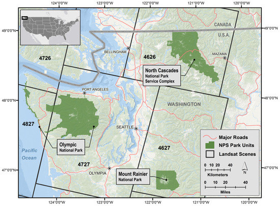
Figure 1.
Study area.
All three parks feature tall peaks or mountain ranges at their core, creating steep precipitation gradients due to the strong rainshadow effects. Annual precipitation on the West side of the parks exceeds 300 cm, decreasing to 60 cm or less to the East. Snow dominates winter precipitation above 1800 m in all the parks, with 8–10 m accumulating on average each winter. Glaciers can be found in each of the parks, forming the headwaters of regionally significant rivers including the Hoh, Skagit, and Nisqually. The Western lowlands in all parks are dominated by mesic Douglas-fir (Pseudotsuga menziesii) and Western hemlock (Tsuga heterophylla) forests which grade to Pacific silver fir (Abies amabilis) forests at middle elevations. The montane silver fir forests transition into mountain hemlock (Tsuga mertensiana) and subalpine fir (Abies lasiocarpa) woodlands and subalpine meadows as elevation increases. Above the upper limit of treeline, alpine meadows segue to rock and ice at the highest elevations. In the Eastern side of the parks, dry forests and woodlands of pine (Pinus spp), Douglas-fir, subalpine fir, and larch (Larix lyallii) predominate.
2.2. Change Detection
To identify and label landscape change, we utilized methods based on those described in Kennedy et al. [5]. The underlying change detection method was LandTrendr, a temporal segmentation algorithm that attempts to characterize durable change in the spectral trajectories of individual pixels over the entire time period of the Landsat Thematic Mapper (TM) sensors [9]. LandTrendr traces the spectral trajectory of each pixel through the time period of the Landsat imagery and uses statistical line-fitting algorithms to break the trajectory into a series of segments. Significant changes in pixel reflectance were marked as inflection points in the yearly trajectory, and from those inflection points we identified the year, magnitude, and duration of change. For this study, we used the normalized burn ratio (NBR) as the spectral index to identify change [10] and mapped change from 1985 to 2009 at North Cascades Complex (NOCA) and Mount Rainier (MORA) and 1985 to 2010 at Olympic (OLYM) National Parks. Following methods described in our original protocol [8], our workflow initially focused on pixel-level changes whose duration was four years or less and whose magnitude of change was at least 10% of the starting index value. Then, once pixels of change were identified, we grouped pixels of the same disturbance year together into disturbance patches, and removed any patches with fewer than nine pixels (less than 0.8 ha). We used Random Forest classification algorithms [11] to assign a category of change to all LandTrendr-generated patches inside the park boundaries following methods described in Kennedy et al. [5]. We summarized the classification results in a series of NPS Natural Resource Data Series reports [12,13,14]. These patches formed the basis of our comparisons.
2.3. Categories of Landscape Change Monitored
We focused on natural disturbances that significantly removed or altered vegetation. This included fires, landslides, avalanches, tree topples, river course alterations, or forest health declines (Table 1, Appendix A). Additionally, we explicitly identified a type of false positive change common in our change detection products. This type of change results when non-durable changes caused by ephemeral phenomena trigger the LandTrendr algorithm to falsely identify a pixel as change, when in fact it was merely subject to unusual phenology, changes in soil moisture, or imperfect masking of shadow or cloud. Consistently found in the subalpine zone of the study area, we labeled this type “Annual Variability.”

Table 1.
List of landscape change types and description.
2.4. Change Label Validation
2.4.1. Office Validation
Following the Random Forest classification, an NPS Geographic Information Systems (GIS) specialist reviewed all change category labels (primary label) inside the park boundaries in the office by using the time series of United States Geological Survey (USGS) and the National Agricultural Imagery Program (NAIP) orthomosaic imagery available in Google Earth™ (Figure 2). The individual park reports list the images used for office validation [12,13,14].

Figure 2.
(a) 2006 Google Earth™ aerial photo used to view pre-disturbance land cover during office validation of a landscape change patch. (b) 2009 Google Earth™ aerial photo used to view post-disturbance land cover of the same patch.
In addition to aerial photography, the analyst performing the office validation visualized the spectral trajectory of a group of pixels surrounding the center of the patch (Figure 3) and viewed the time series of Landsat image chips centered over the patch (Figure 4). The analyst also referenced US Forest Service Insect and Disease Aerial Surveys [15] as an independent data source of areas with affected vegetation.
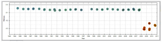
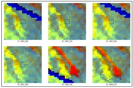
Figure 4.
Pre- and post-disturbance tasseled-cap image chips from the stack of Landsat images used in LandTrendr run. Colors are assigned to the red, green, and blue color hues are tasseled-cap Brightness, Greenness, and Wetness, respectively. Dark blue streaks correspond to Landsat 7 missing scan lines, yellows to broadleaf shrub or tree; red to open soil or rock; light blue and cyan to needle-leaf forest and mixed needle- and broad-leaf forest.
Each patch was also assigned a subjective level of “confidence” in the choice of landscape change label ranging from one (least confident) to three (most confident). In general, we assigned a confidence of three when three criteria were all consistent with expectations for that change category: the visual assessment of the patch size and shape, its spectral trajectory characteristics, and its location on the landscape. We chose a confidence of two when one of the evaluation criteria either did not match the expected pattern or could not be assessed (as with subtle spectral change). Additionally, we assigned a confidence of two when a patch appeared to be mixed: pixels of different change types were combined into the same patch because they were spatially adjacent and occurred during the same year. A confidence of one was assigned when at least two of the evaluation criteria did not match the expected pattern or could not be assessed due to lack of high resolution imagery. If a confidence of two or one was chosen, the analyst recorded a second choice for the patch label (alternative label). In the case of a mixed patch, the primary label was given to the change category that occupied more than 50% of the patch.
2.4.2. Field Validation
Random Sample
Following office labeling, a subset of the patches in each park from the years 2006–2010 was randomly chosen for field validation using the Alaska Pak tool in ArcGIS [17]. Most patches were located within a 500 m buffer of accessible trails and roads and within 5 km of a trailhead. Our previous work has demonstrated that this restricted area of inference is representative of the larger study area. Some change types such as Mass Movements, occurred infrequently during our analysis period. For these rare change types, we expanded the sample further than 500 meters from trails and roads in order to have a minimum of five patches. Fire patches were not included in the field validation of randomly selected patches because we could use existing NPS data to identify them reliably [18]. While the map dataset went back to 1985, we only selected patches from the most recent years for two reasons: (1) vegetation recovery since the time of disturbance can make it difficult to assess the original change agent, and (2) our long-term monitoring protocol repeats periodically, allowing us to evaluate landscape changes every 3–5 years. In 2011–2016 NPS ecologists and/or GIS specialists visited 132 randomly selected patches in the field in all three parks (Figure 5), including 25 patches in MORA, 54 in NOCA, and 53 in OLYM. Field crews were only provided information about the location and the year of the disturbance. A Garmin GPS unit was used to navigate to a Landsat pixel near the center of the patch. In cases where distance or barriers such as streams or steep slopes prevented a field visit, but the patch could be accurately located on the landscape from a nearby vantage point, the field team collected data from a distance. Twenty-eight (21.3 %) of patches were assessed from a distance. Photos were taken of each patch. Confidence in the type was recorded using the same scale as the office validation. Patches with a single, clear change category were assigned a confidence of three. Mixed patches, where evidence of more than one change type was present, and patches where the field team was not sure if the observed change on the ground would have been picked up by satellite overhead because of canopy cover, were assigned a confidence of two. Patches with more than two change types present were assigned a confidence of one. An alternative label was recorded for patches with lower confidence levels. In the case of a mixed patch, the primary label was given to change category that occupied more than 50% of the patch.
Incidental Field Observations
As field sampling is expensive and time consuming, during field-work, we opportunistically extended our dataset by sampling any change patch from 2006–2010 that was accessible on the route to the target random sample. Through this process, we added another 134 patches that we named “incidental samples” (Figure 5). While the incidental samples do not meet requirements for design-based sampling, their selection depended entirely on the random arrangement of change patches along access routes and was not affected by human preference. Given the cost in reaching the randomly-selected plots, the addition of these plots provided an opportunity to double our dataset size. In our later analysis, we treat these samples both separately and combined, and allow the reader to judge the degree to which they add useful information.
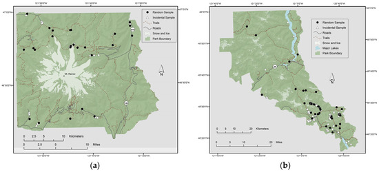
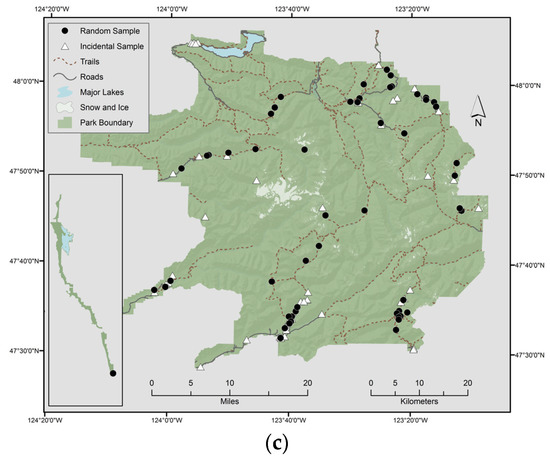
Figure 5.
Selected landscape change patches visited at (a) Mount Rainier National Park, WA, (b) North Cascades National Park Service Complex, WA, and (c) Olympic National Park, WA. Target patches were chosen at random from patches that were up to 500 m from roads or trails. Incidental samples were encountered while accessing the random samples.
See Appendix A for examples of field photos and corresponding office validation materials for each landscape change type.
2.5. Data Analysis
We used a series of agreement matrices to assess how frequently the office label differed from the field label for each of the change categories and sample types. We first compared the office and field labels for the random sample using only primary labels from both field and office, i.e. the alternative label was not considered. We then repeated the process for a dataset that included both random and incidental observations to determine if the general patterns noted for the random plots held. A second matrix was generated for randomly-selected plots that considered both primary and alternative labels to determine a label match. In this case, if one of the primary or alternative office labels matched one of the primary or alternative field labels, the combination was considered a match. While the agreement matrix uses the same format as a contingency matrix, one significant difference in this application is that one view is not considered “truth” and the other the “observation”; therefore, we do not apply labels like “user’s accuracy” and “producer’s accuracy.”
Finally, we examined agreement matrices with respect to confidence values of office and field labels to determine how confidence was distributed between the two validation types and among change categories.
3. Results and Discussion
3.1. Random sample
Office- and field-assigned change category labels for randomly selected patches had an overall agreement of 88.5% (Table 2). Most change categories had a high degree of agreement (> 85%) between office and field labels. The Riparian category had the highest agreement, likely because this category has the most spatially and spectrally discrete signal and a clear landscape context. The Annual Variability, Avalanche, and Mass Movement categories all had levels of agreement above 85%, with Annual Variability showing agreement above 90%. Avalanche and Mass Movement patches were easily recognizable in the field and in the office based on landscape position and the quality of vegetation disturbance associated with them (see Table 1). Annual Variability was unique among the change categories because it denoted a lack of lasting change on the ground. It was most often identified in the field by eliminating all other categories.
Table 2.
Agreement matrix comparing primary labels assigned in office and field for the random sample only.
Tree Toppling and Progressive Defoliation labels had the lowest agreement and were often confused with each other. Five out of seven patches with a primary field label of Tree Toppling and primary office label of Progressive Defoliation had a secondary field label of Progressive Defoliation. Only one office patch out of seven had Tree Toppling as a second option, but Annual Variability was listed four times. This suggests that the office analyst had difficulty interpreting mild Tree Toppling on aerial photography, but did see subtle change in the spectral signal of the pixel trajectory that signified some type of change in forest canopy.
Detailed evaluation of individual cases of disagreement between the office and field labels for the random sample of patches showed three general patterns.
1. Timing of field visit
We found several instances where the field visit occurred after a later disturbance event had superseded the disturbance event of interest, resulting in the field crew evaluating the wrong event. This was the case for one disagreement in the Riparian category, with Fire occurring after the change was detected by the mapping algorithm, but before the field sampling occurred. The sequence of disturbance could easily be discerned when looking at the time series of aerial photos, but was not evident in the field. A similar scenario took place where an Avalanche path was later covered by debris from a Mass Movement, confusing identification in the field.
2. Labeling of process as opposed to result
This category of disagreement includes patches where there may have been some confusion between identifying the cause and effect of landscape change being labeled. From the office view, the analyst usually only sees the effect of change: reduced canopy vigor (Progressive Defoliation), for example, or fallen trees (Tree Topple). During field sampling, however, one might be able to more readily identify the cause of change by looking at what happened under the canopy: reduced canopy vigor having been caused by a small debris flow that covered the base of trees with mud (Mass Movement); or Tree Toppling having been caused by water inundation, killing and toppling the trees (Riparian). The field calls in these cases recorded the cause of change and not the effect as it was visible to the satellite and the analyst in the office. Patches labeled as Progressive Defoliation in the office were most frequently found to have some other disturbance under the canopy. Both cause and effect were often labeled in the field using confidence of two and an alternate agent.
3. Mixed change
This category of disagreement includes patches that had two or more categories of change evident during the field and/or office labeling. Occurrence of several landscape altering events within one year is not distinguishable when using the LandTrendr algorithms, as these utilize a single image per year for change detection, and patches are delineated by combining adjacent pixels labeled with the same year. Therefore, if two separate weather events in the same year caused different categories of change to be adjacent to each other, the resulting patch would contain the effects of both events. Similarly, a single weather event could cause two or more categories of change to occur next to each other if the landscape context was different. This was seen frequently at OLYM and MORA along river corridors after a 2007 winter windstorm event, when riparian flooding and debris flows were seen alongside windthrow patches that caused tree toppling. In both field and office evaluation, such mixed patches were usually labeled with the confidence of two and an alternate category was recorded. When evaluating such labels for agreement, we often found that even though the same categories of change were present in both types of labeling, their order of priority was switched. This was in part caused by different perspectives of field vs. office analysis, where one category appeared to be more prominent under the canopy vs. above, but we also found it difficult to assess the extent of each category of change on the ground when the entire patch was not visible. Indeed, when given the opportunity, we found it easier to label patches in the field when surveying them from afar, especially for certain categories, particularly Progressive Defoliation and Annual Variability.
To determine how the degree of agreement would change if alternative labels were taken into account, we generated a second matrix where labels were considered to be in agreement if either the primary or alternative office label matched either the primary or alternative field label (Table 3). While the disagreement resulting from the timing of the field visit was not improved by this approach, we saw a few of the patches in the other two categories switch to being considered as having a matching label, with the overall agreement increasing to 96.9%. This indicated that the same two categories of change were consistently chosen in office and field, but a different order was used.
Table 3.
Agreement matrix comparing primary and secondary labels assigned in office and field for the random sample only.
3.2. Random and Incidental Sample
We repeated our evaluation using both random and incidental samples and only the primary labels for each patch, and found that the patterns remained largely consistent in this larger dataset (Table 4). Avalanche, Annual Variability, and Mass Movement categories showed agreements similar to that of the random sample. Fire also had a high degree of agreement, with labeling being more confused in the office in cases of lower intensity fires. The accuracy of Progressive Defoliation and Tree Toppling categories improved, with the majority of newly added incidental patches having agreement between office and field labels in these two categories. The Riparian category remained clearly labeled in the field, but slightly less clear in office, with a few patches labeled Avalanche and Tree Toppling.
Table 4.
Agreement matrix comparing primary labels assigned in office and field for both random and incidental samples.
3.3. Evaluation of Confidence Rankings
For the random sample using primary labels only, we evaluated the distribution of the confidence in the labeling (Table 5a,b). For more than 50% of the patches, the field and office analysts shared high confidence. Rarely was the separation of confidence extreme: Only in 4.6% of the patches did the office analyst have lowest confidence and the field analyst highest confidence, and only 1% of the time was the reverse the case. However, there were several areas where confidence scores were close, but not matching: in 12% of the cases, field confidence was lower than in the office, and in 16% of the cases, the reverse was true.
Table 5.
Agreement matrix comparing agreement between office and field confidence levels for primary labels assigned in office and field for the random sample only: (a) raw numbers and (b) percent of sample.
Dissecting these areas of disagreement in confidence paints a more nuanced picture of the relative strengths of the field and the office-based assessments (Table 6 and Figure 6). Progressive Defoliation, Avalanche, and Annual Variability categories had higher percentage of high confidence labels in the office, where Tree Toppling and Mass Movement patches were labeled with more confidence in the field (Table 6). Field analysts had difficulty labeling Annual Variability in the field, with several patches having a confidence of one, largely because the category can only be labeled by eliminating all other categories first, often leaving uncertainty in the choice selection and possibility of other choices (Figure 6). In contrast, the office analyst can utilize landscape position and highly variable spectral trajectory to assign the label of Annual Variability.
Table 6.
Comparison of high and medium confidence levels by change category.
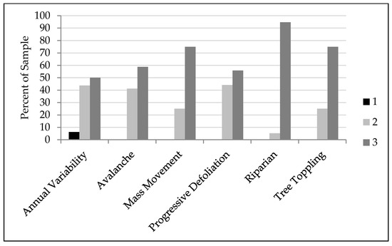
Figure 6.
Distribution of confidence values among change categories for labels assigned in the field for randomly selected patches.
Progressive Defoliation had relatively lower percentage of high confidence labels in both office and field, with a number of plots having the lowest confidence level in the office (Figure 7). Progressive Defoliation is difficult to assess from the office because of the quality and resolution of the one meter NAIP imagery typically used. Orthorectification errors, color balancing, and variable acquisition times all degrade the image quality and make it difficult to visualize the subtle changes in canopy condition detected by LandTrendr for this change type. While assigning labels in the office, altered canopy condition, such as clusters of red needles, are difficult to see in the NAIP. This might encourage the analyst to look for evidence—even subtle or on a fine scale—of any other change spotted in the image, such as broken trees. As with Annual Variability, consulting the spectral trajectory is often helpful, although less so if the change is subtle. In the field, Progressive Defoliation is often hard to see in dense forest where the condition of the canopy is difficult to assess from below and there is no strong evidence of insect or disease.
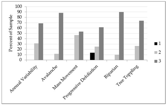
Figure 7.
Distribution of confidence values among change categories for labels assigned in the office for randomly selected patches.
Mass Movements were harder to identify in the office (lower confidence scores), possibly because smaller Mass Movements under canopies were not visible or because the change resulted in secondary change that was visible. Evidence of Mass Movements, such as scattered rock and debris, is easier to see in the field.
While Tree Toppling had a similar distribution of confidence levels in the office and in the field, the reasons for assigning a confidence of two were quite different. In the office, a minor Tree Toppling, with only a few trees down, was hard to identify on aerial photos, and Progressive Defoliation was often assigned as an alternative label. In the field, the Tree Toppling was often seen together with another change category and the confidence of two was assigned because the patch was “mixed.”
4. Conclusions and Recommendations
As computational and algorithmic advances improve our ability to map natural change processes over broad landscapes, the assessment datasets used to evaluate the maps must similarly improve. The cost of conducting field visits to build reference or validation datasets can limit sample size, making methods that are based on aerial photo interpretation conducted in an office setting attractive. This is particularly the case in the large wilderness parks of Washington state, U.S.A., where access for field visitation is time consuming and costly, but where inventories of natural disturbance processes are important to understand landscape dynamics inside and outside protected areas. In order to optimize our validation effort, we compared the relative strengths of field versus office-based validation of landscape change in Mount Rainier, North Cascades Complex, and Olympic National Parks.
In general, we found that the office and field labels strongly agreed. For five of the seven landscape change types we evaluated (Annual Variability, Avalanche, Fire, Mass Movement, and Riparian), the office and field labels had high degree of agreement. For two remaining categories (Progressive Defoliation and Tree Toppling), office-based evaluation of aerial photos was slightly less effective at identifying change, in larger part due to inadequate image resolution. These findings generally held true both for the sample dataset that included only random samples as well as the expanded dataset that included opportunistically acquired samples. Thus, even though we limited our random samples to areas within realistic access from trails and roads, we argue that the underlying change processes represented in our sample form a reasonable representation of the conditions operating more broadly in these parks.
As we explicitly recognized that all interpretation is subject to some uncertainty, we included methods to capture ambiguity and could use those observations to gain a more nuanced understanding of the conditions under which agreement was weaker. Confidence scoring showed that office interpreters had difficulty confidently identifying Tree Toppling and Progressive Defoliation, while field interpreters had difficulty confidently identifying Annual Variability. This is encouraging as these were indeed the categories where those respective interpreters had greater disagreement, suggesting that actual error is related to uncertainty. This is corroborated by the observations of primary and secondary labels: by aggregating primary and secondary labels, the disagreement among these types diminished.
Case by case evaluation of individual plots of disagreement provided further insight into the causes of disagreement. Some errors were introduced in the field sample due to the delay in the time since disturbance and the field visit, emphasizing the importance of doing the field work soon after the disturbance occurred. Some errors were introduced because of the inevitable mismatch between the ground perspective and the office (aerial photograph) perspective. In general, field observations allowed greater understanding of the complexities of the change processes, as could be expected. Indeed, some disagreement occurred when field observers were able to observe the process itself, rather than simply the manifestation of that process visible at the top of the canopy from an aerial photo. However, field observations underneath a canopy may not be able to understand what is occurring at the top of the canopy that could be detectable by the satellite imagery.
Indeed, this raises an important issue to consider whenever designing a validation study. For certain change processes, field visits will be more able to understand the processes involved. However, the downward-looking view afforded by high resolution imagery provides the same perspective as that of the satellite imagery on which the landscape maps are made, and indeed might be more appropriate as a means of corroborating the detection noted by the sensors. When a subtle mass movement under a canopy causes trees to topple, it may be just as appropriate to document the impact as the potential underlying cause. Moreover, it appears that even the cases of disagreement are relatively minor.
In general, we conclude that the magnitude or severity of change is a better indicator of whether or not a field assessment is warranted. More damaging and abrupt categories of change, especially those that remove canopy cover, are more suitable for labeling in the office. More subtle changes and changes in forests that do not remove canopy, such as Progressive Defoliation or a minor Tree Topple, could potentially be checked in the field. However, our results suggest that a field visit may not entirely resolve uncertainty about these subtle types of change.
Our work demonstrates that validation of Landsat-derived landscape change patches can be done using office based tools such as aerial imagery, and that such methods provide an adequate validation for most change-types, thus reducing the need for expensive field visits.
Author Contributions
Conceptualization, N.A., C.C. and R.K.; methodology, C.C.; software, R.K.; validation, C.C. and N.A.; formal analysis, C.C.; investigation, N.A. and C.C.; resources, R.K.; data curation, N.A.; writing—original draft preparation, C.C.; writing—review and editing, N.A and R.K.; visualization, N.A.; supervision, C.C..; project administration, C.C.; funding acquisition, C.C, N.A and R.K.
Funding
This research was funded by the National Park Service Inventory and Monitoring program. Kennedy was funded through task agreement J8W07110003 to Cooperative Ecosystem Study Unit agreement H8W07110001.
Acknowledgments
Shelby Clary assisted with office validation and John Boetsch and Katherine Beirne helped with field sampling.
Conflicts of Interest
The authors declare no conflict of interest. The funders had no role in the design of the study; in the collection, analyses, or interpretation of data; in the writing of the manuscript, or in the decision to publish the results.
Appendix A. Field and Office Validation Examples of Seven Landscape Change Types Assessed in this Study
1. Annual Variability
Annual Variability category was created to be able to model and remove polygons detected by LandTrendr that do not capture change of interest to the NCCN. Usually, these changes are associated with variability in snow cover, clouds, terrain shadows, or vegetation phenology that is not removed in the image processing steps and is of great enough magnitude to pass through filtering. Annual variability patches are generally only found in high elevations areas with subalpine vegetation, such as above the tree line. The interpreter must exercise care in determining a polygon of this class truly shows no change. The TimeSync trajectories of these changes usually show high degree of variability throughout the time period being examined and are dominated by red, brown and orange hues. Figure A1 shows an example of a 2008 patch in Mount Rainier National Park that would be placed in the Annual Variability category. Landsat tasseled-cap image chips between 2006 and 2009 are not significantly different, except for slight variation in hues most likely related to differences in timing of snowmelt and soil moisture during the image acquisition dates.
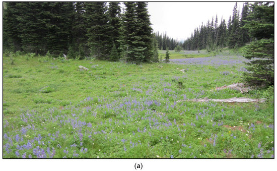
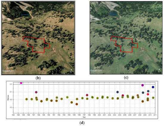
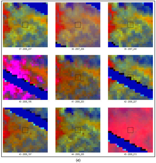
Figure A1.
A 2008 Annual Variability patch generated by LandTrendr at Mount Rainier National Park. (a) Photo collected during field validation. Photo credit: NPS/Catharine Copass (2016). (b) Pre-disturbance 2006 aerial photo as viewed in Google Earth™. (c) Post-disturbance 2009 aerial photo as viewed in Google Earth™. (d) TimeSync spectral trajectory of nine pixels around patch centroid. (e) Part of the series of tasseled-cap image chips covering pre- and post-disturbance years as viewed in TimeSync. Dark blue streaks in (e) correspond to Landsat 7 missing scan lines, magenta colors correspond to snow and bright red colors denote clouds.
2. Avalanche
Avalanches originate in snow receiving zones on ridges or high on the valley wall. They are typically long, linear patches, although some events can be broken up into multiple smaller patches depicting areas of greatest removal of vegetation. If the avalanche occurred in an existing avalanche chute, the TimeSync trajectory usually starts in bright greens and yellows, which are representative of low statured, mostly broadleaf vegetation—small conifers, deciduous shrubs and herbs. If swaths of forest were removed, the TimeSync trajectory will start as greenish blue, representative of mature conifer forest. As avalanches typically remove some but not all of the vegetation, the trajectory after the event is typically shown in hues of red, brown and tan. Higher magnitude avalanches occasionally traverse the valley floor and leave a large pile of downed trees in their wake, which can usually be seen in the aerial photography. Figure A2 shows field and office validation components for a large avalanche that occurred at North Cascades National Park in 2008.
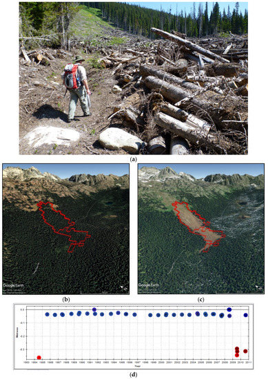
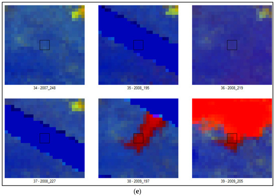
Figure A2.
A 2008 Avalanche patch generated by LandTrendr at North Cascades National Park. (a) Photo collected during field validation. Photo credit: NPS/ Chris Lauver (2011). (b) Pre-disturbance 2006 aerial photo as viewed in Google Earth™. (c) Post-disturbance 2009 aerial photo as viewed in Google Earth™. (d) TimeSync spectral trajectory of nine pixels around patch centroid. (e) Part of the series of tasseled-cap image chips covering pre- and post-disturbance years as viewed in TimeSync. Dark blue streaks in (e) correspond to Landsat 7 missing scan lines and bright red (as opposed to darker red) color in the last image chip denotes clouds.
3. Fire
Figure A3 shows a 2004 fire at Mount Rainier National Park. Fires tend to leave standing trees with no foliage, which can be seen in the aerial photography as thin shadows. Fire polygons are often large. Some lower intensity fires leave behind a mix of dead and singed trees. Sometimes active burning and smoke can been seen in the aerial photography, since the aerial photos in the Pacific Northwest are usually taken in August. The trajectory in the TimeSync usually shows changing from blue and green of conifers to a mix of brighter colors where the vegetation has been completely burned, to orange for shrubby new growth (Figure A3c).
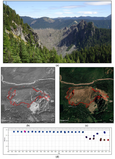
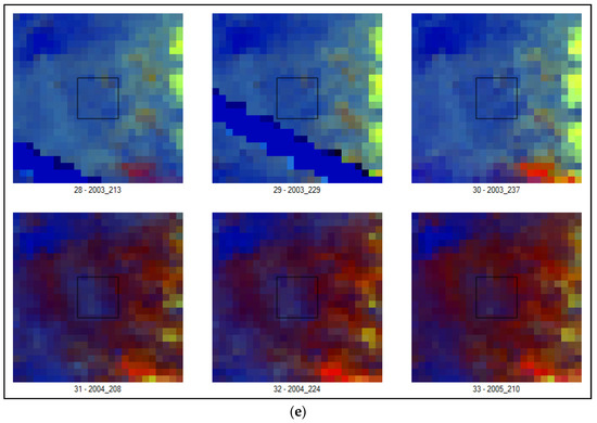
Figure A3.
A 2004 Fire patch generated by LandTrendr at Mount Rainier National Park. (a) Photo collected during field validation. Photo credit: NPS/ Natalya Antonova (2016). (b) Pre-disturbance 2003 aerial photo as viewed in Google Earth™. (c) Post-disturbance 2006 aerial photo as viewed in Google Earth™. (d) TimeSync spectral trajectory of thirty six pixels around patch centroid. (e) Part of the series of tasseled-cap image chips covering pre- and post-disturbance years as viewed in TimeSync. Dark blue streaks in (e) correspond to Landsat 7 missing scan lines.
4. Mass Movement
This category includes a variety of vegetation-removing changes that expose rock or bare ground. Larger events are typically called landslides, and are found on valley walls away from streams or creeks. Most landslides totally remove vegetation and are often persistent, such as the 2004 Goodell Creek landslide shown in Figure A4. Some rare events, however, are better described as “soil creeps” or “slumps” and are characterized by only partial removal of vegetation. Debris flows are mass movements associated with water discharge, such as streams. Mass movements are distinguished from the riparian category in that they occur on valley walls, perpendicular to the valley floor. Riparian category is associated with changes found on the valley floor, along low gradient rivers. Mass movements are distinguished from avalanches by the magnitude of change: mass movement leaves little to no vegetation; and by shape and context. The interpreters usually look for persistent red and orange colors in the TimeSync trajectory following the event (Figure A4c).
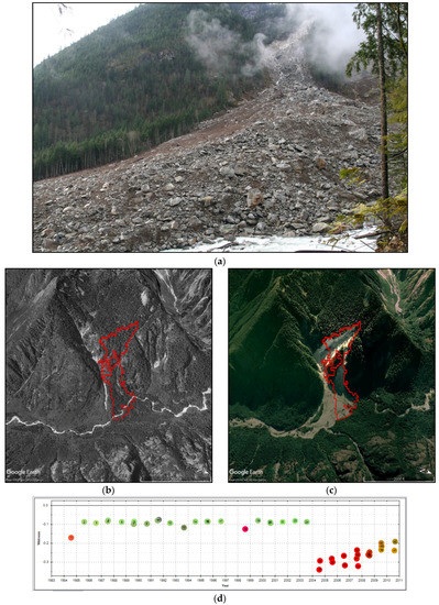
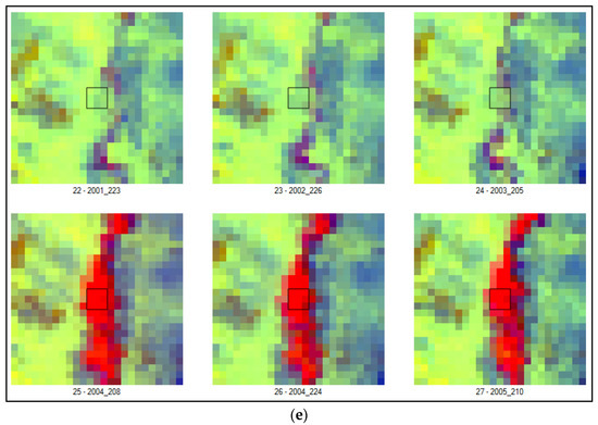
Figure A4.
A 2004 Mass Movement patch generated by LandTrendr at North Cascades National Park. (a) Photo collected during field validation. Photo credit: NPS/ Jon Riedel (2004). (b) Pre-disturbance 1998 aerial photo as viewed in Google Earth™. (c) Post-disturbance 2006 aerial photo as viewed in Google Earth™. (d) TimeSync spectral trajectory of nine pixels around patch centroid. (e) Part of the series of tasseled-cap image chips covering pre- and post-disturbance years as viewed in TimeSync.
5. Progressive Defoliation
Figure A5 shows components of field and office validation for 2003 North Cascades National Park patch that falls into the Progressive Defoliation category. This category is usually assigned to landscape change polygons where forest cover still remains but has undergone slow changes in spectral values that represent a loss of greenness and wetness (Figure A5c). Interpreting the color change in TimeSync is therefore more challenging. The interpreter usually sees a very slight dip in the trajectory with decrease in blueness and greenness. However, the decrease is not big enough to suggest change from conifer to broadleaf vegetation or bare earth (Figure A5).
The decreasing greenness of the forest can be difficult to discern in the aerial photography. In some stands the decline is due to LandTrendr detecting individual trees which have completely died. These dead trees appear in the aerial photos as bright red or yellow. In some stands the decline is due to the tip and top limbs of a significant proportion of the trees succumbing to some pathogen. This type of decline shows up as a subtle greying of the canopy in the aerial photos and can be hard to discern if the color balance of the photos is poor. In addition, change polygons in this category can have both types of declining trees.
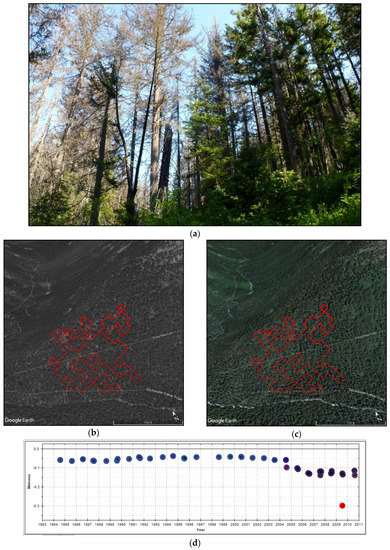
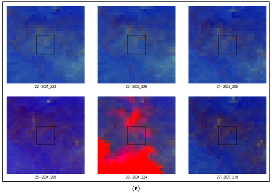
Figure A5.
A 2003 Progressive Defoliation patch generated by LandTrendr at North Cascades National Park. (a) Photo collected during field validation. Photo credit: NPS/ Chris Lauver (2011). (b) Pre-disturbance 1998 aerial photo as viewed in Google Earth™. (c) Post-disturbance 2013 aerial photo as viewed in Google Earth™. (d) TimeSync spectral trajectory of thirty six pixels around patch centroid. (e) Part of the series of tasseled-cap image chips covering pre- and post-disturbance years as viewed in TimeSync. Bright red color in (e) the last image chip corresponds to clouds.
6. Riparian
Riparian patches are restricted to the valley floor where the gradient is much lower and the valley floor is wider. Typical riparian patches show areas where either conifer or broadleaf vegetation previously existed and have been converted to either active river channel, with water, or river bank, with gravel and sediment. Figure A6 shows a 2006 Riparian landscape patch from Mount Rainier National Park with evident tree mortality and gravel and sediment depositions. The spectral trajectories of these changes show either sudden increase in wetness or brightness, depending on the resulting cover type. These changes are usually easily identified on aerial photos and Landsat image chips (Figure A6b–d).
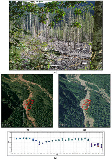
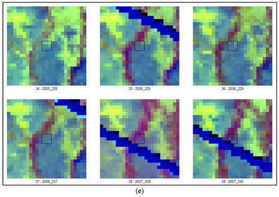
Figure A6.
A 2007 Riparian patch generated by LandTrendr at Mount Rainier National Park. (a) Photo collected during field validation. Photo credit: NPS/ Natalya Antonova (2016). (b) Pre-disturbance 2006 aerial photo as viewed in Google Earth™. (c) Post-disturbance 2009 aerial photo as viewed in Google Earth™. (d) TimeSync spectral trajectory of nine pixels around patch centroid. (e) Part of the series of tasseled-cap image chips covering pre- and post-disturbance years as viewed in TimeSync. Dark blue streaks in (e) correspond to Landsat 7 missing scan lines.
7. Tree Toppling
The Tree Toppling category primarily includes forest areas where the trees have been both broken off and toppled to the ground in major wind events. This category is rare at NOCA and MORA. It is more common at OLYM, especially in the Quinault, Hoh, and Queets River valleys on the west side of the park and also in the northeast corner of the park. Figure A7 shows a large 2008 Tree Toppling patch that resulted from the December 2007 Great Coastal Gale [19]. This category also includes areas where the Tree Toppling is due to root rot - the structural outcome is similar and the agent is typically hard to determine just from the imagery. Large Tree Toppling events can build on themselves, with subsequent events occurring in the vicinity of the original patch. TimeSync trajectory of these events often shows some green vegetation remaining after the toppling, either because some of the trees are still standing or the foliage of the downed trees is not completely dead (Figure A7d). Down tree trunks are often visible on the aerial photograph. Windthrow events usually occur in areas on the landscape that are exposed to wind, either on top of ridges and knolls or along rivers.
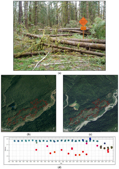
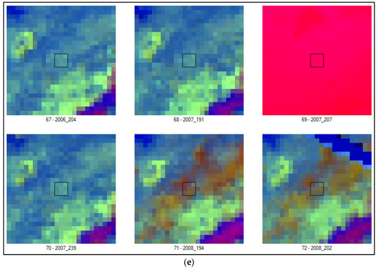
Figure A7.
A 2008 Tree Toppling patch generated by LandTrendr at Olympic National Park. (a) Photo collected during field validation. Photo credit: NPS (2008). (b) Pre-disturbance 2006 aerial photo as viewed in Google Earth™. (c) Post-disturbance 2009 aerial photo as viewed in Google Earth™. (d) TimeSync spectral trajectory of nine pixels around patch centroid. (e) Part of the series of tasseled-cap image chips covering pre- and post-disturbance years as viewed in TimeSync. Dark blue streaks in (e) correspond to Landsat 7 missing scan lines and bright red color corresponds to clouds.
References
- Hansen, M.C.; Potapov, P.V.; Moore, R.; Hancher, M.; Turubanova, S.A.; Tyukavina, A.; Thau, D.; Stehman, S.V.; Goetz, S.J.; Loveland, T.R.; et al. High-Resolution Global Maps of 21st-Century Forest Cover Change. Science 2013, 342, 850–853. [Google Scholar] [CrossRef] [PubMed]
- Masek, J.G.; Goward, S.N.; Kennedy, R.E.; Cohen, W.B.; Moisen, G.G.; Schleeweis, K.; Huang, C. United States forest disturbance trends observed using Landsat time series. Ecosystems 2013, 16, 1087–1104. [Google Scholar] [CrossRef]
- Cohen, W.B.; Yang, Z.; Kennedy, R.E. Detecting trends in forest disturbance and recovery using yearly Landsat time series: 2. TimeSync—Tools for calibration and validation. Remote Sens. Environ. 2010, 114, 2911–2924. [Google Scholar] [CrossRef]
- McDermid, G.J.; Franklin, S.E.; LeDrew, E.F. Remote sensing for large-area habitat mapping. Prog. Phys. Geogr. 2005, 29, 449–474. [Google Scholar] [CrossRef]
- Kennedy, R.E.; Yang, Z.; Braaten, J.; Copass, C.; Antonova, N. Attribution of disturbance change agent from Landsat time-series in support of habitat monitoring in the Puget Sound region, USA. Remote Sens. Environ. 2015, 166, 271–285. [Google Scholar] [CrossRef]
- Kirschbaum, A.A.; Pfaff, E.; Gafvert, U.B. Are U.S. national parks in the Upper Midwest acting as refugia? Inside vs. outside park disturbance regimes. Ecosphere 2016, 7, 1–15. [Google Scholar] [CrossRef]
- Bey, A.; Diaz, A.S.P.; Maniatis, D.; Marchi, G.; Mollicone, D.; Ricci, S.; Bastin, J.F.; Moore, R.; Federici, S.; Rezende, M.; et al. Collect Earth: Land Use and Land Cover Assessment through Augmented Visual Interpretation. Remote Sens. 2016, 8, 807. [Google Scholar] [CrossRef]
- Antonova, N.; Copass, C.; Kennedy, R.K.; Yang, Z.; Braaten, J.; Cohen, W. Protocol for Landsat-Based Monitoring of Landscape Dynamics in North Coast and Cascades Network Parks: Version 2; Natural Resource Report NPS/NCCN/NRR—2012/601; National Park Service: Fort Collins, CO, USA, 2012.
- Kennedy, R.E.; Yang, Z.; Cohen, W.B. Detecting trends in forest disturbance and recovery using yearly Landsat time series: 1. LandTrendr—Temporal segmentation algorithms. Remote Sens. Environ. 2010, 114, 2897–2910. [Google Scholar] [CrossRef]
- Key, C.H.; Benson, N.C. Landscape assessment: Remote sensing of severity, the Normalized Burn Ratio. In FIREMON: Fire Effects Monitoring and Inventory System; Lutes, D.C., Ed.; USDA Forest Service, Rocky Mountain Research Station: Ogden, UT, USA, 2005. [Google Scholar]
- Breiman, L. Random forests. Mach. Learn. 2001, 45, 5–32. [Google Scholar] [CrossRef]
- Antonova, N.; Copass, C.; Clary, S. Landsat-Based Monitoring of Landscape Dynamics in the North Cascades National Park Service Complex: 1985–2009; Natural Resource Data Series; NPS/NCCN/NRDS—2013/532; National Park Service: Fort Collins, CO, USA, 2013.
- Antonova, N.; Copass, C.; Clary, S. Landsat-Based Monitoring of Landscape Dynamics in Mount Rainier National Park: 1985–2009; Natural Resource Data Series; NPS/NCCN/NRDS—2014/637; National Park Service: Fort Collins, CO, USA, 2014.
- Copass, C.; Antonova, N.; Clary, S. Landsat-Based Monitoring of Landscape Dynamics in Olympic National Park: 1985–2010; Natural Resource Data Series; NPS/NCCN/NRDS—2016/1053; National Park Service: Fort Collins, CO, USA, 2016.
- United States Forest Service (USFS). Insect and Disease Aerial Detection Surveys. Geospatial Dataset. Available online: https://www.fs.usda.gov/detail/r6/forest-grasslandhealth/insects-diseases/?cid=stelprdb5286951 (accessed on 18 September 2018).
- Crist, E.P.; Cicone, R.C. A physically-based transformation of Thematic Mapper data—The TM tasseled cap. IEEE Trans. Geosci. Remote Sens. 1984, GE22, 256–263. [Google Scholar] [CrossRef]
- Sarwas, R. NPS AlaskaPak 3.0 Software. National Park Service, 2011. Available online: https://irma.nps.gov/DataStore/Reference/Profile/2176910 (accessed on 7 December 2018).
- National Park Service (NPS). NPS—Wildland Fire Map Service. Geospatial Dataset; National Park Service and Sundance Consulting Inc.—National Interagency Fire Center: Boise, ID, USA, 2018.
- Read, W. The Great Coastal Gale of 2007. Available online: http://www.climate.washington.edu/stormking/December2007.html (accessed on 18 August 2018).
© 2018 by the authors. Licensee MDPI, Basel, Switzerland. This article is an open access article distributed under the terms and conditions of the Creative Commons Attribution (CC BY) license (http://creativecommons.org/licenses/by/4.0/).