Laplacian Regularized Spatial-Aware Collaborative Graph for Discriminant Analysis of Hyperspectral Imagery

Abstract

Dimensionality Reduction (DR) models are of significance to extract low-dimensional features for Hyperspectral Images (HSIs) data analysis where there exist lots of noisy and redundant spectral features. Among many DR techniques, the Graph-Embedding Discriminant Analysis framework has demonstrated its effectiveness for HSI feature reduction. Based on this framework, many representation based models are developed to learn the similarity graphs, but most of these methods ignore the spatial information, resulting in unsatisfactory performance of DR models. In this paper, we firstly propose a novel supervised DR algorithm termed Spatial-aware Collaborative Graph for Discriminant Analysis (SaCGDA) by introducing a simple but efficient spatial constraint into Collaborative Graph-based Discriminate Analysis (CGDA) which is inspired by recently developed Spatial-aware Collaborative Representation (SaCR). In order to make the representation of samples on the data manifold smoother, i.e., similar pixels share similar representations, we further add the spectral Laplacian regularization and propose the Laplacian regularized SaCGDA (LapSaCGDA), where the two spectral and spatial constraints can exploit the intrinsic geometric structures embedded in HSIs efficiently. Experiments on three HSIs data sets verify that the proposed SaCGDA and LapSaCGDA outperform other state-of-the-art methods.

1. Introduction

As one of the most significant remote sensing techniques, Hyperspectral Images (HSIs) captured by modern remote sensors have been successfully applied in real-world tasks, such as target detection, and crop yield estimation, etc. [1,2,3]. Typically, each pixel in HSIs consists of hundreds of spectral bands/features, which means that HSIs can provide more abundant information about remote sensing objects than multispectral and typical color images with few bands/features, thus HSI classification has attracted much attention in the last several decades. Although many classification models have been introduced, such as Support Vector Machine (SVM), Deep Learning (DL), and Representation based Classification [4,5,6,7], etc., the curse of dimensionality problem stemming from the high-dimensional features/bands could largely compromise the performance of various classification algorithms, especially when there are only small number of labeled training data. Therefore, many Dimensionality Reduction (DR) methods have been introduced to preprocess the HSI data so that the noisy and redundant features can be removed and the discriminative features can be extracted in low-dimensional subspace. To some extent, DR has become fundamental for HSI data analysis [8,9,10,11,12].

Generally speaking, all DR models for HSIs can be divided into two categories: bands selection and feature extraction [8,12]. The former focuses on choosing representative subset from original spectral bands with physical meanings by some criteria, while the latter tries to learn new features by transforming observed high-dimensional spectral bands/features to the low-dimensional features with discriminative and structural information. As stated in [8], discovering optimal bands from enormous numbers of possible band combinations by feature selection methods is typically suboptimal, thus in this paper we only focus on feature extraction based DR methods for HSIs instead of feature selection.

The past decades have witnessed that various feature extraction algorithms have been introduced for HSI data analysis. There are roughly two major classes of DR techniques for feature extraction, the linear and nonlinear DR models. Principal Components Analysis (PCA) may be the most classic linear DR method, which tries to linearly project observed data into the low-dimensional subspace where the data variance is maximized. To further extend PCA into the Bayesian framework, Probabilistic PCA (PPCA) [13] was also proposed. Other PCA extensions include Kernel PCA (KPCA), Robust PCA, Sparse PCA, and Tensor PCA, etc. [14,15,16,17,18]. However, the linear assumption in PCA indicates that PCA and its extensions could fail when there are nonlinear structures embedded into the high-dimensional observations. Thus, many nonlinear DR models have been developed, among which DR models based on manifold learning could be representative because they could be able to capture the intrinsic nonlinear structures (e.g., multiple clusters, subspace structure and manifolds) in observed data with high dimensionality [12,19,20].

Most manifold learning based DR techniques try to model the local geometric structures of data based on graph theory [19,21]. The performance of these manifold learning based methods mainly depends on the following two aspects: (i) the design of the similarity graphs, and (ii) the embedding of new test data—the out-of-sample problem. For the first factor, different methods have distinct ideas to construct similarity graph matrices, such as Local Linear Embedding (LLE), Laplace Eigenmap (LE), Neighborhood Preserving Embedding (NPE), and Locality Preserving Projection (LPP) [19,22], etc. In [19], a general Graph Embedding (GE) framework was introduced to unify these existing manifold learning algorithms where various methods to construct different similarity graph matrices were compared. Lunga et al. [20] also reviewed typical manifold learning based DR methods for HSI classification. Recently, the representation based approaches have also been introduced to manifold learning framework to constitute the similarity graphs [12]. For example, Sparse Representation (SR), Collaborative Representation (CR) and Low Rank Representation (LRR) [7] were utilized to construct the sparse graph (${\ell }_1$ graph), collaborative graph (${\ell }_1$ graph) and low-rank graph, giving rise to Sparsity Preserving Projection (SPP) [23], Collaborative Representation based Projection(CRP) [24] and Low Rank Preserving Projections (LRPP) [25], respectively. For the second aspect, in order to address the out-of-sample problem encountered by many manifold learning models, extra mappings that project new samples to low-dimensional manifold subspace were added into existing manifold learning algorithms, where linear mapping was typically utilized like LPP and NPE [19].

The aforementioned techniques are unsupervised DR models, which means that extra labels cannot be utilized even if they are available in HSIs data where we are typically given some labels. By making use of these label information, the unsupervised DR methods can be extended to the supervised settings, which could improve the discriminating power of DR models. Linear Discriminant Analysis (LDA) can be representative in the line. Compared to its linear counterpart PCA, LDA performs DR by maximizing the between-class scatter and minimizing the within-class scatter simultaneously, leading to more discriminative dimensionality-reduced features than PCA. However, LDA and its extensions including Generalized Discriminant Analysis (GDA) suffer from the limitation of extracting maximum $C-1$ features with C being the number of label classes [8] and the Small-Sample-Size (SSS) problem. Nonparametric Weighted Feature Extraction (NWFE) and its kernel extension Kernel NWFE address these issues by using the weighted means to evaluate the nonparametric scatter matrices, resulting in more than $C-1$ features being learned [8]. Other LDA extensions include Regularized LDA (RLDA) [26] and Modified FLDA (MFLDA) [27].

PCA was also extended to supervised versions to handle the extra labels such as Supervised PPCA (SPPCA) [16]. However, these methods are most likely incapable of discovering complex nonlinear geometric structure in numerous HSIs spectral features, which could deteriorate the performance of DR models. Therefore, many supervised manifold learning models which are capable of capturing the local geometric structure of neighboring pixels have been developed, such as Supervised LPP (SLPP) [19], Local Fisher Discriminant Analysis (LFDA) [28] and local graph discriminant embedding (LGDE) [29]. The most easy way to realize supervised manifold learning models is to construct the similarity graph matrices based on neighboring samples belonging to the same class. Alternatively, representation based models have been extended into the supervised settings, such as Sparse Graph-based Discriminate Analysis (SGDA) [30], Weighted Sparse Graph-based Discriminate Analysis (WSGDA) [31], Collaborative Graph-based Discriminate Analysis (CGDA) [32], Laplacian regularized CGDA (LapCGDA) [7], Discriminant Analysis with Graph Learning (DAGL) [33] and Sparse and Low-Rank Graph-based Discriminant Analysis (SLGDA) [34], etc.

To further add nonlinearity to the supervised manifold models, kernel tricks are also utilized, resulting into Kernel LFDA (KLFDA) [28], Kernel CGDA (KCGDA) [32] and Kernel LapCGDA (KLapCGDA) [7], etc. A recent survey in [12] termed these kind of techniques Graph-Embedding Discriminant Analysis, where the basic idea behind these models is to construct various discriminative intrinsic graphs with different criterions, such as ${\ell }_1$ and ${\ell }_2$ graphs employed in SGDA and CGDA, respectively. Although their models have demonstrated the effectiveness for extracting discriminative HSI features in terms of classification accuracy, their performance could become unsatisfactory because of the lack of considering spatial information.

Recently, some researchers have shown that spatial information in HSIs could be efficiently utilized to boost the DR models, leading to the joint spectral-spatial DR techniques where most of these kinds of models can be roughly divided into two classes as stated in [35]:

(i)

Spectral-Spatial information can be used as a preprocessing. For example, Gaussian weighted local mean operator was employed to extract spectral-spatial feature in Composite Kernels Discriminant Analysis (CKDA) [36]. A robust spectral-spatial distance rather than simple spectral distance was adopted in Robust Spatial LLE (RSLLE) [37]. A local graph-based fusion (LGF) [38] method was proposed to conduct DR by simultaneously considering the spectral information and the spatial information extracted by morphological profiles (MPs). Recently, Tensor PCA (TPCA) [18], deep learning based models [5], superpixels [29,39] and propagation filter [40] techniques were also successfully utilized to extract the spectral-spatial features.

(ii)

Spectral-spatial information can be used as a spatial constraint/regularization. For instance, the authors of [41] proposed a Spatial and Spectral Regularized Local Discriminant Embedding (SSRLDE) where the local similarity information was encoded by a spectral-domain regularized local preserving scatter matrix and a spatial-domain local pixel neighborhood preserving scatter matrix. Spectral-Spatial LDA (SSLDA) [42] made use of a local scatter matrix constructed from a small neighborhood as a regularizer which makes the samples approximate the local mean in the low-dimensional feature space among the small neighborhood. The Spectral-Spatial Shared Linear Regression (SSSLR) [35] made use of a convex set to describe the spatial structure and a shared structure learning model to learn a more discriminant linear projection matrix for classification. Spatial-spectral hypergraph was used in Spatial-Spectral Hypergraph Discriminant Analysis (SSHGDA) [43] to construct complex intraclass and interclass scatter matrices to describe the local geometric similarity of HSI data. Superpixel-level graphs and local reconstruction graphs were constructed to be the spatial regularization in Spatial Regularized LGDE (SLGDE) [29] and Local Geometric Structure Fisher Analysis (LGSFA) [44], respectively. Recently, He et al. [45] reviewed many state-of-the-art spectral-spatial feature extraction and classification methods, which demonstrates that spatial information could be beneficial to HSI feature extraction and classification.

In this paper, we focus on the Graph-Embedding Discriminant Analysis framework because of its outstanding performance and low complexity. Although some progress has been made based on this framework, such as SGDA, CGDA, LapCGDA, and SLGDA, etc., the performance of these models could be further improved by efficiently incorporating the spatial information into the framework. Motivated by recently introduced Joint CR (JCR) [46] and Spatial-aware CR (SaCR) [10] algorithms, in this paper, we propose the Spatial-aware Collaborative Graph-based Discriminate Analysis (SaCGDA) where spatial-spectral features are firstly preprocessed by the average filtering in JCR and then the spatial information is encoded as a spatial regularization item in CR to construct the spectral-spatial similarity graph in an easy and efficient way. To further improve the performance of the model, inspired by LapCGDA, the spectral Laplacian regularization item is also introduced into SaCGDA, giving rise to the Laplacian regularized SaCGDA (LapSaCGDA) which makes use of the spectral-spatial information more effectively.

The rest of the paper is organized as follows. In Section 2, we briefly review the related works, including the Collaborative Representation(CR) and the Graph-Embedding Discriminant Analysis framework. The proposed SaCGDA and LapSaCGDA will be introduced in Section 3. Then, three HSI datasets are used to evaluate the effectiveness of the newly proposed algorithms in Section 4. Finally, the concluding remarks and comments will be given in Section 5.

2. Related Works

In this section, we will review some related works, including the typical CR models and its variants JCR and SaCR, plus the Graph-Embedding Discriminant Analysis framework.

For the sake of consistency, we make use of the following notations throughout this paper: $X=[{\mathit{x}}_1,\dots ,{\mathit{x}}_N]$ are observed (inputs) data with each sample ${\mathit{x}}_n$ in a high-dimensional space ${\mathcal{R}}^D$; $\mathit{y}=[y_1,\dots ,y_N]$ are observed (outputs or labels) data with each point $y_n$ being discrete class label in $\{1,2,\dots ,C\}$, where C is the number of the classes; $Z=[{\mathit{z}}_1,\dots ,{\mathit{z}}_N]$ are the dimensionality-reduced variables/features in a low-dimensional space ${\mathcal{R}}^d$ ($d\ll D$) with each ${\mathit{z}}_n$ corresponding to ${\mathit{x}}_n$ and/or ${\mathit{y}}_n$. For the sake of convenience, we further denote X as an $D\times N$ matrix, $\mathit{y}$ an $N\times 1$ vector and Z an $d\times N$ matrix, so the training data can be defined as $\mathcal{D}={\left\{({\mathit{x}}_n,y_n)\right\}}_{n=1}^N$. Let $n_l$ be the number of training data from l-th class and ${\sum }_{l=1}^C{n}_l=N$. Similar to LDA, the goal of discriminant analysis based DR models is to find the low-dimensional projection Z with typical linear mapping

$$\begin{array}{c}\hfill Z=P^{T}X,\end{array}$$

(1)

where the transformation matrix $P\in {\mathcal{R}}^{D\times d}$ linearly projects each sample ${\mathit{x}}_n$ to the low-dimensional subspace.

2.1. Collaborative Representation (CR)

The representation based models such as Sparse Representation (SR), Collaborative Representation (CR) and Low-Rank Representation(LRR) have been successfully applied in many tasks [7]. Compared to the computationally expensive SR, CR can provide comparative classification performance with very efficient closed-form solution to learn the model parameters. Given a test sample ${\mathit{x}}^{*}$, all the training data are employed to represent it by

$$\begin{array}{c}\hfill L\left(\mathit{w}\right)=\left|\right|{\mathit{x}}^{*}-X\mathit{w}{\left|\right|}_2^2+\alpha \mathsf{\Omega }\left(\mathit{w}\right),\end{array}$$

(2)

where the the regularization parameter $\alpha$ balances the trade-off between the reconstruction residual and the regularization of the representation coefficients. Typically, ${\ell }_2$ norm is used with $\mathsf{\Omega }\left(\mathit{w}\right)={\left|\right|\mathit{w}\left|\right|}_2^2$. However, other regularization methods can also be adopted [47,48]. For example, ${\ell }_1$ instead of ${\ell }_2$ norm brings the sparsity of the coefficient, resulting in SR. A locality regularization [49] $\mathsf{\Omega }\left(\mathit{w}\right)={\left|\right|\mathsf{\Gamma }\mathit{w}\left|\right|}_2^2$ provides different freedom to training data according to the Euclidean distances from ${\mathit{x}}^{*}$, where each diagonal entry in the diagonal matrix $\mathsf{\Gamma }$ is defined by

$$\begin{array}{c}\hfill {\mathsf{\Gamma }}_{ii}=\left|\right|{\mathit{x}}^{*}-{\mathit{x}}_i{\left|\right|}_2,(i=1,2,\dots ,N).\end{array}$$

(3)

For classic CR model, be solving the the least-squares problem, the optimal representation coefficients ${\mathit{w}}^{*}$ can be easily obtained with closed-form solution

$$\begin{array}{c}\hfill w^{*}={(X^{T}X+\alpha I)}^{-1}{X}^T{x}^{*}\end{array}$$

(4)

and then the class label of test sample ${\mathit{x}}^{*}$ can be predicted according to the minimum residual

$$\begin{array}{c}\hfill label\left({\mathit{x}}^{*}\right)=\underset{l=1,2,\dots ,C}{argmin}{\parallel {\mathit{x}}^{*}-X_l{\mathit{w}}_l^{*}\parallel }_2^2,\end{array}$$

(5)

where $X_l$ and ${\mathit{w}}_l^{*}$ are the subsets of X and ${\mathit{w}}^{*}$ corresponding to specific class label l, respectively.

As we have mentioned that spatial information is significant for HSI data analysis. Two simple but efficient CR models have been recently developed. The first one termed by Joint CR (JCR) makes use of the spatial information as a preprocessing based on the fact that the neighboring pixels usually share similar spectral characteristics with high probability. Thus, the spatial correlation across neighboring pixels could be indirectly incorporated by a joint model, where each training and testing sample is represented by spatially averaging its neighboring pixels that is similar with the convolution operation in Convolution Neural Network (CNN). Another model called joint Spatial-aware CR (JSaCR) further utilizes the spatial information as a spatial constraint in a very easy and effective way

$$\begin{array}{c}\hfill L\left(\mathit{w}\right)=\parallel {\tilde{\mathit{x}}}^{*}-\tilde{X}{\mathit{w}\parallel }_2^2+\alpha \parallel \tilde{\mathsf{\Gamma }}{\mathit{w}\parallel }_2^2+\beta {\parallel \mathrm{diag}\left(\mathit{s}\right)\mathit{w}\parallel }_2^2,\end{array}$$

(6)

where ${\tilde{\mathit{x}}}^{*}$ and each element in $\tilde{X}$ are the average spectral features for the test sample ${\mathit{x}}^{*}$ and each training point ${\mathit{x}}_n^{*}$ centered in a small window with m neighbors, respectively, $\tilde{\mathsf{\Gamma }}$ is similarly defined by $\widetilde{{\mathsf{\Gamma }}_{ii}}=\left|\right|{\tilde{\mathit{x}}}^{*}-{\tilde{\mathit{x}}}_i{\left|\right|}_2(i=1,2,\dots ,N)$, each element in $s=[s_1,s_2,\dots ,s_N]$ is associated with each training sample, which encourages that representation coefficients $\mathit{w}$ are spatially coherent w.r.t. the training data, $\mathrm{diag}\left(\mathit{s}\right)$ is a square diagonal matrix with the elements of vector $\mathit{s}$ on the main diagonal. To further explain the spatial constraint in the third term in Equation (6), let us firstly denote the pixel coordinate of the testing sample ${\mathit{x}}^{*}$ and each training pixel ${\mathit{x}}_n$ by $(p_{*},q_{*})$ and $(p_n,q_n)$, respectively. The spatial relationship between them can be simply measured by smooth parameter t

$$\begin{array}{c}\hfill {\mathit{s}}_n={\left[\mathrm{dist}((p_n,q_n),(p_{*},q_{*}))\right]}^t,\end{array}$$

(7)

where $\mathrm{dist}(·,·)$ represents the Euclidean distance with smooth parameter t adjusting the distance decay speed for the spatial constraint. Actually, the normalized element $s\in (0,1]$ is obtained by dividing $max\left(\mathit{s}\right)$ from $\mathit{s}$. A large value of t implicitly means that pixels that are spatially far away from the test sample will be penalized by assigning coefficients close to 0. As can be seen from the JSaCR formulation, the locality constraint (second term) and spatial constraint (third term) are controlled by the regularization parameters $\alpha$ and $\beta$, respectively.

2.2. Graph-Embedding Discriminant Analysis

Graph-Embedding Discriminant Analysis [12] seeks to learn the projection matrix P based on the linear model assumption ${\mathit{z}}_n=P^T{\mathit{x}}_n$ by preserving the similarities of samples in the original observation space. Many manifold learning models and discriminant analysis based methods can be unified into this framework, such as LPP, NPE, LDA and recently proposed SGDA, CGDA, etc.

Typically, a general Graph-Embedding Discriminant Analysis model can be formulated by finding a low-dimensional subspace where the local neighborhood relationships in the high-dimensional observations can be retained. Based on typical linear mapping ${\mathit{z}}_n=P^T{\mathit{x}}_n$, the objective function of Graph-Embedding Discriminant Analysis is

$$\begin{array}{cc}\hfill \tilde{P}& =\underset{P}{argmin}\sum _{i\ne j}\parallel {\mathit{z}}_i-{\mathit{z}}_j\parallel W_{ij}=\underset{P}{argmin}\sum _{i\ne j}\parallel P^T{\mathit{x}}_i-P^T{\mathit{x}}_j\parallel W_{ij}\hfill \\ & =\underset{P}{argmin}trace\left(P^{T}XL{X}^{T}P\right),s.t.P^{T}X{L}_P{X}^{T}P=I,\hfill \end{array}$$

(8)

where the similarity graph matrix W is built on pairwise distances between observed samples to represent local geometry with each $W_{ij}$ being the similarity/affinity between samples ${\mathit{x}}_i$ and ${\mathit{x}}_j$, $L=T-W$ is the Laplacian matrix of graph G, T is the diagonal matrix with nth diagonal element being $T_{ii}={\sum }_{j=1}^N{W}_{ij}$ and $L_p$ is a sample scale normalization constraint or some Laplacian matrix of penalty $G_p$. By simply re-formulating the objective function as

$$\begin{array}{c}\hfill \tilde{P}=\underset{P}{argmin}\frac{|P^{T}XL{X}^{T}P|}{|P^{T}X{L}_p{X}^{T}P|}.\end{array}$$

(9)

The optimal projection matrix P can be obtained by solving a generalized eigenvalue decomposition problem

$$\begin{array}{c}\hfill XL{X}^{T}P=\lambda X{L}_p{X}^{T}P,\end{array}$$

(10)

where $P\in {\mathcal{R}}^{D\times d}$ is constructed by the d eigenvectors corresponding to the d smallest nonzero eigenvalues. As can be seen from the formulations, the performance of Graph-Embedding Discriminant Analysis algorithms largely depends on the construction methods of the similarity/affinity matrix.

Let’s firstly take the unsupervised LPP model as the classic example where the similarity between two samples ${\mathit{x}}_i$ and ${\mathit{x}}_j$ is typically measured by the heat kernel if they are the neighbors

$$\begin{array}{c}\hfill W_{ij}=e^{-\frac{\parallel {\mathit{x}}_i-{\mathit{x}}_j{\parallel }^2}{r}},\end{array}$$

(11)

with a pre-specified parameter r.

Compared to unsupervised LPP, supervised discriminant analysis models like LDA, SGDA and CGDA construct the similarity matrix in the supervised manner, which could provide better discriminant ability. For example, W in LDA, SGDA or CGDA is typically expressed by a block-diagonal matrix

$$\begin{array}{c}\hfill \left[\begin{array}{cccc}{W}^1& & & \\ & W^2& & \\ & & \ddots & \\ & & & W^C\end{array}\right],\end{array}$$

(12)

where each ${\left\{W^l\right\}}_{l=1}^C$ is the within-class similarity matrix of size $n_l\times n_l$ based on $n_l$ training samples only from the l-th class. Different strategies have been applied to construct the within-class similarity matrix. As can be seen from Equation (13) ${\ell }_1$, ${\ell }_2$, $nuclear+{\ell }_1$ and $manifold+{\ell }_2$ norms are adopted in SGDA, CGDA, SLGDA and LapCGDA, respectively, using the representation based algorithms to construct the similarity matrix $W^l=[{\mathit{w}}_1^l;{\mathit{w}}_2^l;\dots ;{\mathit{w}}_{n_l}^l]\in {\mathcal{R}}^{n_l\times n_l}$ with each $n_l$ being the number of training data only from l-th class:

$$\begin{array}{c}\mathrm{SGDA}:\underset{{\mathit{w}}_n^l}{argmin}\parallel {\mathit{x}}_n^l-X_n^l{\mathit{w}}_n^l{\parallel }_2^2+\alpha {\parallel {\mathit{w}}_n^l\parallel }_1,\hfill \end{array}$$

(13)

$$\begin{array}{c}\mathrm{CGDA}:\underset{{\mathit{w}}_n^l}{argmin}\parallel {\mathit{x}}_n^l-X_n^l{\mathit{w}}_n^l{\parallel }_2^2+\alpha {\parallel {\mathit{w}}_n^l\parallel }_2,\hfill \end{array}$$

(14)

$$\begin{array}{c}\mathrm{SLGDA}:\underset{{\mathit{w}}_n^l}{argmin}\parallel {\mathit{x}}_n^l-X_n^l{\mathit{w}}_n^l{\parallel }_2^2+\alpha \parallel {\mathit{w}}_n^l{\parallel }_{*}+\beta {\parallel {\mathit{w}}_n^l\parallel }_1,\hfill \end{array}$$

(15)

$$\begin{array}{c}\mathrm{LapCGDA}:\underset{{\mathit{w}}_n^l}{argmin}\parallel {\mathit{x}}_n^l-X_n^l{\mathit{w}}_n^l{\parallel }_2^2+\alpha {\parallel {\mathit{w}}_n^l\parallel }_2+\beta {\mathit{w}}_{\mathit{n}}^{\mathit{l}}T{H}_n{\mathit{w}}_n^l,\hfill \end{array}$$

(16)

where ${\mathit{x}}_n^l$ is a training sample from l-th class, $X_n^l$ denotes all training samples from l-th class but excluding ${\mathit{x}}_n$, ${\parallel ·\parallel }_{*}$ in SLGDA indicates the nuclear norm, and $H_n$ in LapCGDA is the Laplacian matrix constructed by Equation (11).

Although these models have demonstrated their effectiveness, their performance could be unsatisfactory because the spatial information in HSIs is not utilized. Compared to the spatial constraints like local reconstruction points, superpixel and hypergraph based spatial regularization models in LGSFA [44], SLGDE [29] and SSHGDA [43], the simple spatial prior in JSaCR has been proven to be fast and efficient. Therefore, in this paper, we introduce the spatial prior into CGDA model because of its outstanding performance and low complexity.

3. Laplacian Regularized Spatial-Aware CGDA

In this section, motivated by JSaCR and LapCGDA, we propose Laplacian regularized Spatial-Aware CGDA (LapSaCGDA) by simultaneously introducing spatial prior and spectral manifold regularization into CGDA which will significantly increase the discriminant ability of the learnt similarity/affinity matrix and then boost the performance of the DR model.

Firstly, based on the fact that the average filtering in JCR could smooth the random noises in HSI data, we similarly preprocess all the HSI data, which leads to the new notations such as ${\tilde{\mathit{x}}}_n$ and $\tilde{X}$, meaning a training sample and all training data after the preprocessing, respectively.

Then, based on the JSaCR model in Equation (6), it is straightforward to make use of JSaCR instead of typical CR in CGDA to construct the within-class similarity matrix ${\left\{W^l\right\}}_{l=1}^C$ for $n_l$ labeled samples belonging to l-th class by

$$\begin{array}{c}\hfill \underset{{\mathit{w}}_n^l}{argmin}\parallel {\tilde{\mathit{x}}}_n^l-\widetilde{X_n^l}{\mathit{w}}_n^l{\parallel }_2^2+\alpha \parallel \tilde{\mathsf{\Gamma }}{\mathit{w}}_n^l{\parallel }_2^2+\beta {\parallel \mathrm{diag}\left({\mathit{s}}_n\right){\mathit{w}}_n^l\parallel }_2^2,\end{array}$$

(17)

where ${\tilde{\mathit{x}}}_n^l$ is a preprocessed training sample from l-th class, $X_n^l$ are all preprocessed training samples from l-th class but excluding ${\tilde{\mathit{x}}}_n$, $\tilde{\mathsf{\Gamma }}$ and $\mathit{s}$ are similarly defined by $\widetilde{{\mathsf{\Gamma }}_{ii}}={\parallel {\tilde{\mathit{x}}}_n^l-{\tilde{\mathit{x}}}_i^l\parallel }_2$ and ${\mathit{s}}_n={\left[\mathrm{dist}((p_n,q_n),(p_i,q_i))\right]}^t$ with the pixel coordinate $(p_i,q_i)$ for samples in l-th class $(i=1,2,\cdots ,n_l)$, respectively.

It is easy to obtain the closed-form solution for the optimization problem in Equation (17) by

$$\begin{array}{c}\hfill {\mathit{w}}_n^l={({\widetilde{X_n^l}}^T\widetilde{X_n^l}+\alpha \tilde{\mathsf{\Gamma }}+\beta \mathrm{diag}\left({\mathit{s}}_n\right))}^{-1}{\widetilde{X_n^l}}^T{\tilde{\mathit{x}}}_n^l.\end{array}$$

(18)

As stated in JSaCR, the locality prior (second term) and spatial prior (third term) in Equation (17) can be efficient to extract the spectral-spatial structure in HSI data. However, the simple locality prior w.r.t. the second term in Equation (17) could be inefficient to exploit the intrinsic geometric information compared to manifold priors like the Laplacian regularization used in LapCGDA. Hence, we further propose the Laplacian regularized Spatial-Aware CGDA (LapSaCGDA) by introducing the Laplacian regularization into SaCGDA. In order to compare the two spectral priors, we simply add the spectral Laplacian constraint into SaCGDA as the third regularization instead of replacing the spectral locality constraint in SaCGDA with the spectral Laplacian constraint.

Similar to SaCGDA, the within-class similarity matrix ${\left\{W^l\right\}}_{l=1}^C$ of LapSaCGDA can be constructed by solving the following optimization problem:

$$\begin{array}{c}\hfill \underset{{\mathit{w}}_n^l}{argmin}{\parallel {\tilde{\mathit{x}}}_n^l-\widetilde{X_n^l}{\mathit{w}}_n^l\parallel }_2^2+\underset{\mathrm{spectral}\mathrm{locality}\mathrm{constraint}}{\underbrace{\alpha \parallel \tilde{\mathsf{\Gamma }}{\mathit{w}}_n^l{\parallel }_2^2}}+\underset{\mathrm{spatial}\mathrm{constraint}}{\underbrace{\beta \parallel \mathrm{diag}\left({\mathit{s}}_n\right){\mathit{w}}_n^l{\parallel }_2^2}}+\underset{\mathrm{spectral}\mathrm{Laplacian}\mathrm{constraint}}{\underbrace{\gamma {\mathit{w}}_{\mathit{n}}^{\mathit{l}}T{H}_n{\mathit{w}}_n^l}},\end{array}$$

(19)

where $H_{ni}=e^{-\frac{\left|\right|{\tilde{\mathit{x}}}_n^l-{\tilde{\mathit{x}}}_i^l{\left|\right|}^2}{r}}$ with a pre-specified parameter r.

Mathematically, the closed-form solution for this optimization can be obtained by

$$\begin{array}{c}\hfill {\mathit{w}}_n^l={({\widetilde{X_n^l}}^T\widetilde{X_n^l}+\alpha \tilde{\mathsf{\Gamma }}+\beta \mathrm{diag}\left(\mathit{s}\right)+\gamma H_n)}^{-1}{\widetilde{X_n^l}}^T{\tilde{\mathit{x}}}_n^l.\end{array}$$

(20)

It is worth noting that LapSaCGDA could reduce to SaCGDA when $\gamma =0$, to LapCGDA when $\beta =0$ or to CGDA when $\beta =0$ and $\gamma =0$, thus the proposed LapSaCGDA model is very general and can unify the three models with different regularization parameters’ configurations.

After obtaining all the within-class similarity matrix ${\left\{W^l\right\}}_{l=1}^C$ by SaCGDA or LapSaCGDA, the block-diagonal similarity matrix $W=diag(W^1,W^2,\dots ,W^C)$ can be simply constructed like Equation (12). Finally, based on the Graph-Embedding Discriminant Analysis framework, it is easy to evaluate the optimal projection matrix P by solving the eigenvalue decomposition in Equation (10).

The complete LapSaCGDA algorithm is outlined in Algorithm 1.

Algorithm 1 LapSaCGDA for HSIs Dimensionality Reduction and Classification

Input:  High-dimensional training samples $X\in {\mathcal{R}}^{D\times N}$, training ground truth $y\in {\mathcal{R}}^N$, pre-fixed latent dimensionality d, and testing pixels $X^{*}\in {\mathcal{R}}^{D\times M}$, testing ground truth $y^{*}\in {\mathcal{R}}^M$, a pre-specified regularization parameters $\alpha ,\beta ,\gamma$. Output:  s = {$Acc$, P}.  1: Preprocess all the training and testing data by average filtering;  2: Evaluate the similarity matrix W by solving Equation (20);  3: Evaluate the optimal projection matrix P by solving the eigenvalue decomposition in Equation (10);  4: Evaluate low-dimensional features for all the training and testing data by ${\mathit{z}}_n=P^T{\mathit{x}}_n$;  5: Perform KNN and/or SVM in low-dimensional feature space and return classification accuracy $Acc$;  6: returns

As for the model complexity, Algorithm 1 tells us that, compared to other contrastive models like CGDA and LapCGDA, the proposed SaCGDA and LapSaCGDA do not increase the complexity except the average filtering preprocessing step, which could be conducted before the algorithm starts.

4. Experiments

In this section, we will validate the effectiveness of the proposed SaCGDA and LapSaCGDA for HSI feature reduction and classification. The novel model is compared to the classic supervised DR models NWFE [8], SPPCA [16], plus recently developed DR techniques LapCGDA [7], SLGDA [34], and LGSFA [44] based on the Graph-Embedding Discriminant Analysis framework in three typical HSI datasets in terms of classification accuracy. In addition, the classic SVM is also applied in the original high-dimensional spectral feature space for comparison. Since all the HSIs datasets are initially preprocessed by the average filtering, the original spectral features can be regarded as the spectral-spatial features as well.

For a fair comparison, firstly all the data will be preprocessed by average filtering with a $7\times 7$ spatial window, and then K-Nearest Neighbors (KNN) with Euclidean distance and SVM with Radial Basis Function (RBF) kernel are chosen as the classifiers in the dimensionality-reduced space for verifying all the DR models in terms of the classification Overall Accuracy (OA), the classification Average Accuracy (AA) and the Kappa Coefficient (KC) as well as the True Positive Rate (TPR) and False Positive Rates (FPR). The parameter K in KNN is set to be 5, and the optimal parameters of kernel in SVM are selected by the tenfold cross-validation with a given set $\{0.001,0.01,0.1,1,10,100,1000,10000\}$. The regularization parameters such as $\alpha ,\beta ,\gamma$ in LapCGDA, SLGDA, and the proposed SaCGDA and LapSaCGDA will be chosen by the grid search with a given set $\{{10}^{-6},{10}^{-5},\dots ,{10}^4\}$ firstly. Then, as the optimal projection dimensionality for each DR model has to be pre-specified before model optimization, for each piece of HSI data, where the same training and testing data are randomly picked, we compare and choose the best dimensionality of each DR model in the range of 1–30 in terms of the classification accuracy based on KNN in the projected low-dimensional feature space. Finally, with the selected optimal dimensionality for each piece of HSI data and each DR algorithm, we further compare all the DR techniques as the number of training data increases. Classification maps are also compared when limited training data are available. All the experiments are repeated ten times and the averaged results are reported with standard deviation (STD).

4.1. Data Description

Three HSIs datasets including Pavia University scene, Salinas scene and Indian Pines scene from [50] are employed in our experiments.

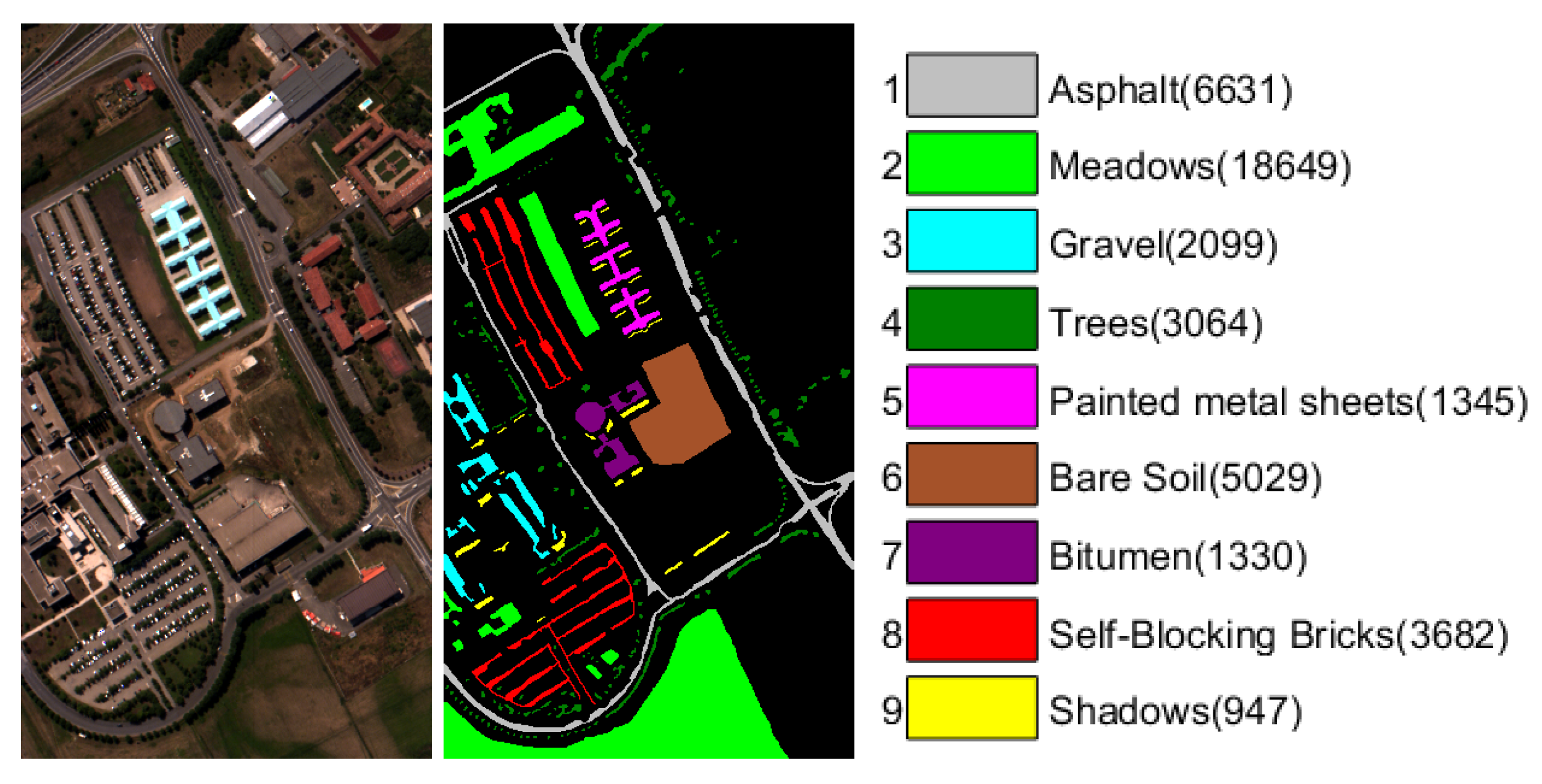
The Pavia University scene (PaviaU) is captured by the sensor known as the Reflective Optics System Imaging Spectrometer (ROSIS-3) over the Pavia University, Italy in 2002. The number of spectral bands is 103 with the image resolution of $610\times 340$ pixels after removing some pixels without information and noise bands. The geometric resolution is $1.3$ m. The data set contains nine land cover types, and the False Color Composition (FCC) and Ground Truth (GT) are shown in Figure 1.

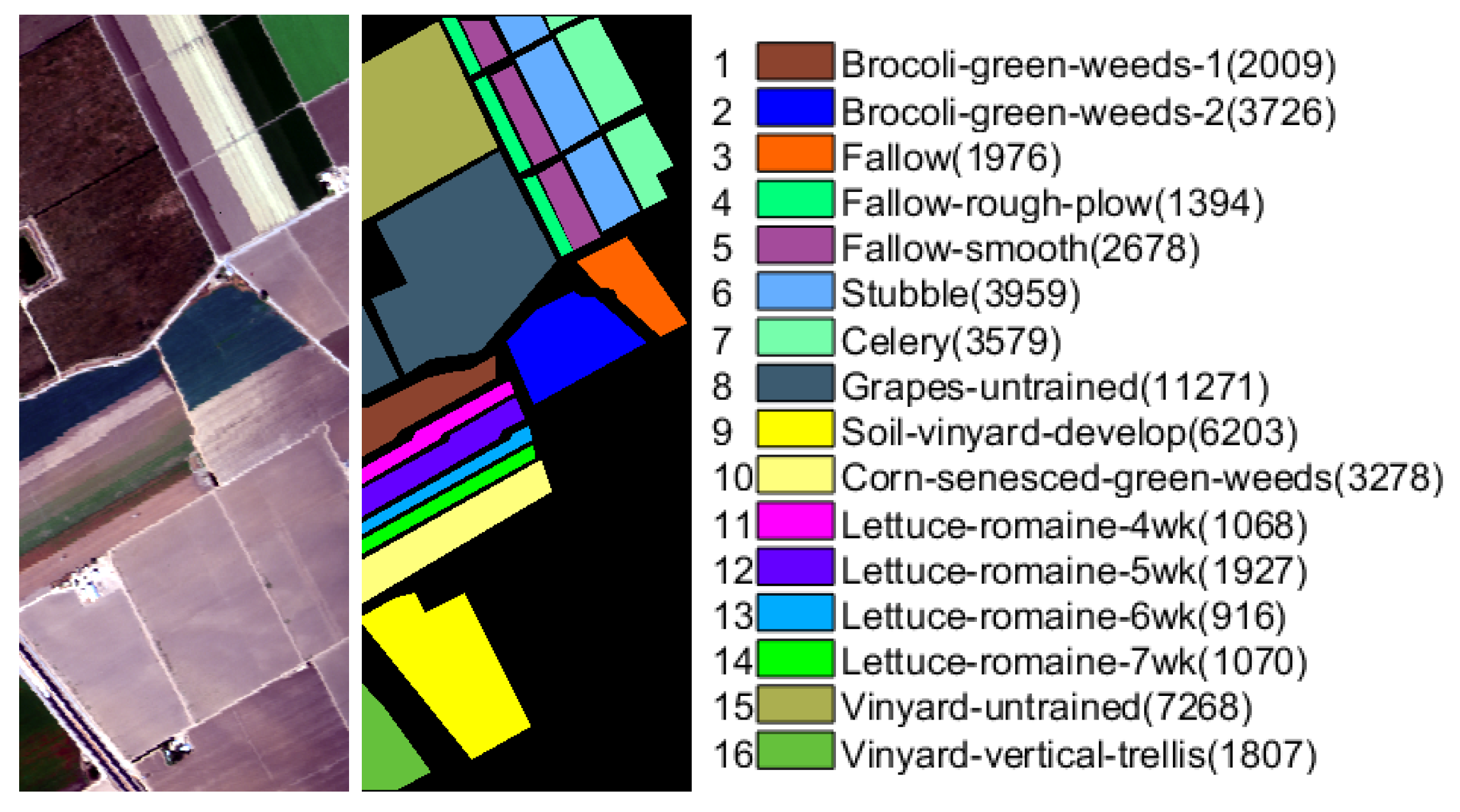
The Salinas scene (Salinas) was collected by an Airborne Visible/Infrared Imaging Spectrometer (AVIRIS) sensor over Salinas Valley, California in 1998 with the geometric resolution of $3.7$ m. The spatial size of this data is $512\times 217$ pixels with 224 spectral bands. After removing 20 water absorption and atmospheric effects bands, the number of spectral band becomes 204. Sixteen ground truth classes are labeled in this data set, and the false color composition and ground truth are shown in Figure 2.

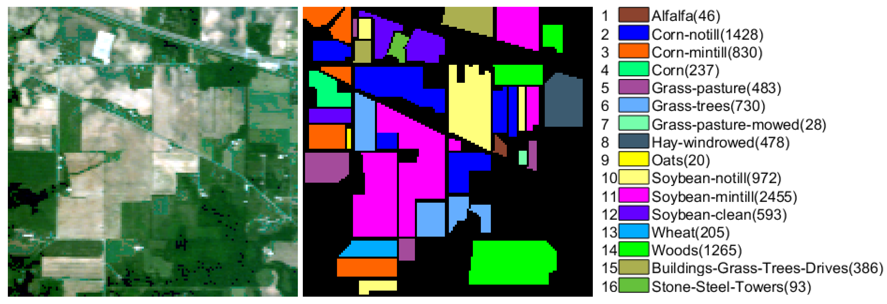
The Indian Pines data (IndianPines) is a scene from Northwest Indiana captured by the AVIRIS sensor in 1992, which consists of $145\times 145$ pixels and 200 spectral bands after removing bands with noise and water absorption phenomena. Sixteen ground truth classes are considered in this data set, and the false color composition and ground truth are shown in Figure 3.

4.2. Experiments on the Pavia University Data

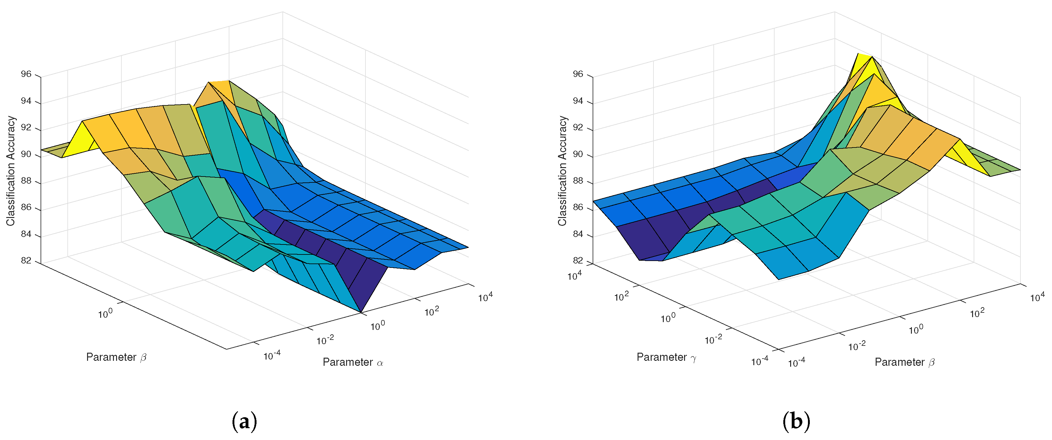
In order to demonstrate the effectiveness of the proposed models, initially, we analyze the parameters’ sensitivity and select optimal parameters for each DR model because the regularization parameters such as $\alpha ,\beta ,\gamma$ in LapCGDA, SLGDA, and the proposed SaCGDA and LapSaCGDA significantly affect the performance of the DR models. In addition, for the proposed SaCGDA and LapSaCGDA, the smooth parameter t in the spatial prior is also optimally searched in the set $\{2,4,6,8\}$. In the experiment, 30 samples are randomly picked from each class as training data and the projection dimensionality is fixed to 30 so that the parameters’ sensitivity analysis can be conducted.

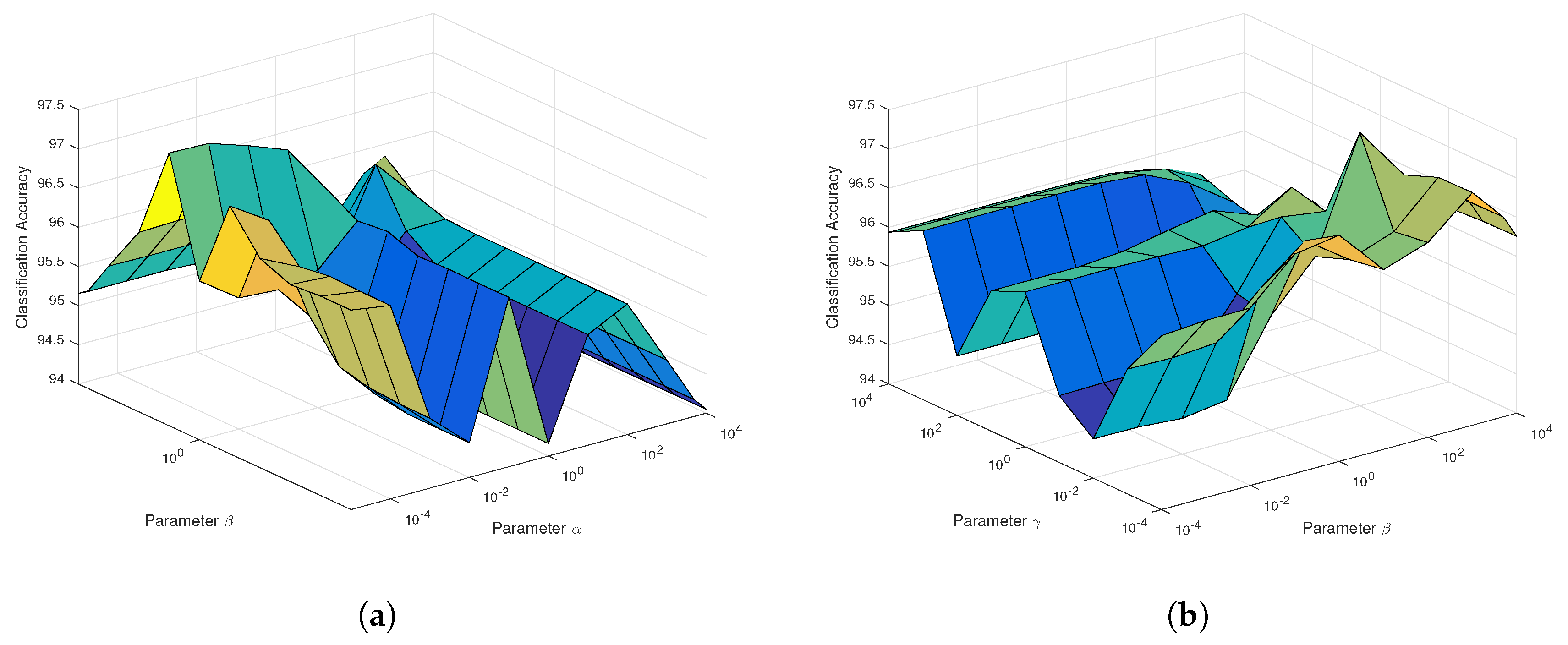
As can be seen from Figure 4a for SaCGDA, the optimal parameter $\beta$ w.r.t. the spatial prior significantly affects the OAs compared to the parameter $\alpha$ w.r.t. the spectral locality prior, and the best smooth parameter t in the spatial prior is 2 in our experiment. Similar results can also be found in the parameters’ sensitivity experiment for LapSaCGDA, which are not completely shown in Figure 4b because it is difficult to plot the 4D figure w.r.t. three parameters. Here, we simply set the parameter $\alpha =0.0001$ w.r.t. the spectral locality prior for both SaCGDA and LapSaCGDA because OAs are insensitive to parameter $\alpha$ based on the experimental results of parameters’ sensitivity. The best regularization parameters for LapCGDA, SLGDA, SaCGDA and LapSaCGDA are listed in

Table 1. Optimal parameters settings for LapCGDA, SLGDA, SaCGDA and LapSaCGDA on the Pavia University data.

Model	$\mathit{\alpha }$	$\mathit{\beta }$	$\mathit{\gamma }$
LapCGDA	0.1	100	—
SLGDA	10	10	—
SaCGDA	0.0001	100	—
LapSaCGDA	0.0001	1000	0.01

, which will be used in the following experiments. In addition, what can be found from Figure 4b and Table 1 is that the best parameter $\gamma$ w.r.t. the spectral manifold prior in LapSaCGDA is larger than the optimal parameter $\alpha$ w.r.t. the spectral locality prior, meaning that the manifold prior has more influence on the DR model than the simple locality prior.

Based on these optimal parameters selected by the grid search, we further choose the best dimensionality of the projection space in terms of the OAs based on KNN and SVM performed in the low-dimensional projection space. The best number of dimensionality of the embedding space will be chosen from the range of 1–30.

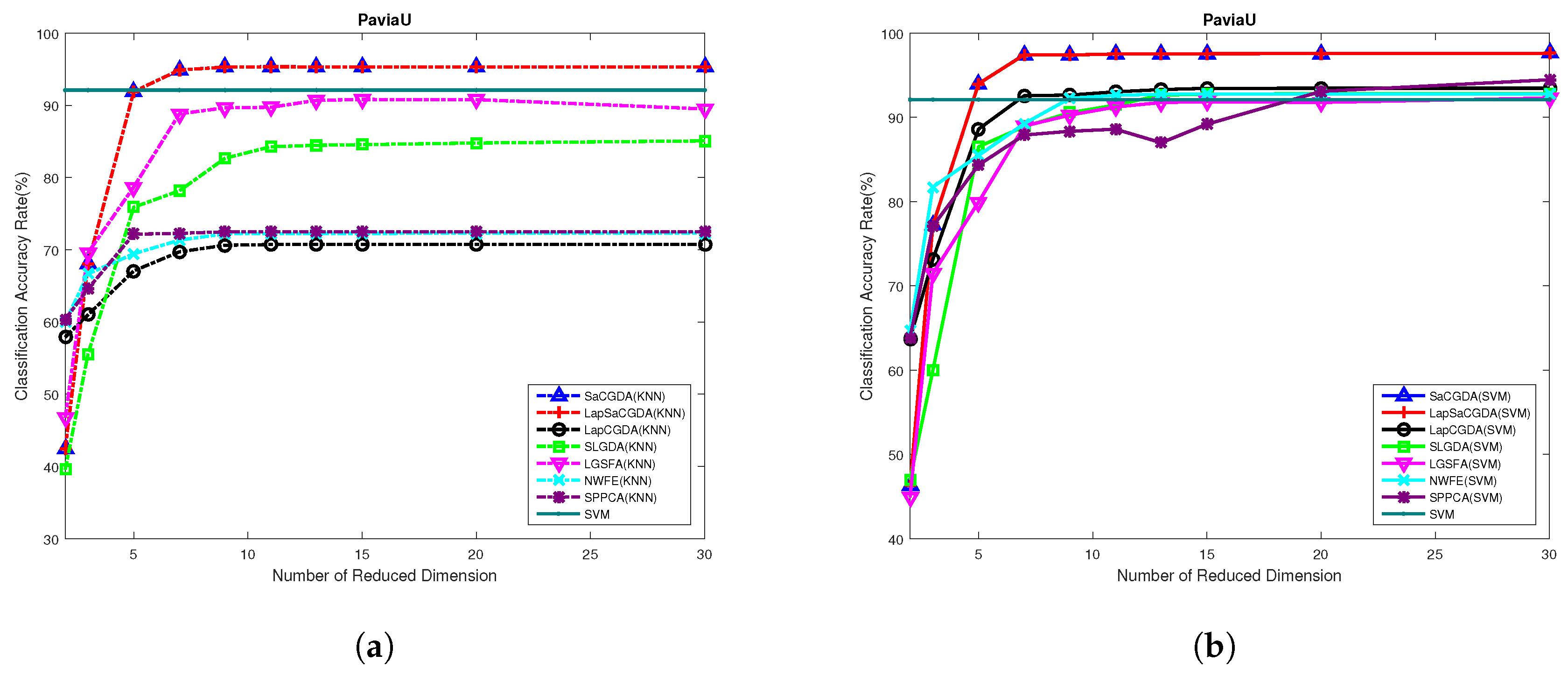
What can be seen from Figure 5 is that the proposed SaCGDA and LapSaCGDA outperform other DR models in almost all low-dimensional projection spaces, and the optimal number of dimensionality for each DR model in this HSI data is 30. It also should be highlighted that, in the low-dimensional projection space, the OAs based on KNN from the proposed SaCGDA and LapSaCGDA outperform SVM based on original high-dimensional features significantly, meaning the that the learned low-dimensional features are very discriminatory.

Furthermore, we also show the experimental results when different numbers of training data are randomly chosen. In addition, 20–80 samples are randomly chosen from each class, and the remainder are for testing. It can be viewed from

Table 2. Classification results with different amounts of training data on the Pavia University data (OA ± STD (%)).

Classifier	DR Model	${\mathit{n}}_{\mathit{l}}=20$	${\mathit{n}}_{\mathit{l}}=40$	${\mathit{n}}_{\mathit{l}}=60$	${\mathit{n}}_{\mathit{l}}=80$
KNN	SPPCA	69.58 ± 1.79	76.67 ± 3.27	81.53± 2.57	84.34 ± 2
	NWFE	69.18 ± 3.34	75.87 ± 2.55	80.93 ± 2.25	83.64 ± 1.32
	SLGDA	78.56 ± 7.05	86.45 ± 1.32	88.73 ± 2.36	91.13 ± 1.45
	LapCGDA	71.74 ± 4.98	78.65 ± 3.75	84.16 ± 1.87	86.32 ± 1.73
	LGSFA	81.8 ± 3.68	89.57 ± 1.32	92.98 ± 0.99	94.67 ± 0.82
	SaCGDA	87.73 ± 4.38	94.81 ± 1.21	96.44 ± 0.78	97.35 ± 0.57
	LapSaCGDA	90.29 ± 1.11	95.23 ± 0.55	96.52 ± 0.37	97.63 ± 0.4
SVM	SPPCA	90.39 ± 2.46	93.33 ± 1.06	94.6± 0.75	95.4 ± 0.36
	NWFE	89.65 ± 1.94	92.55 ± 1.04	94.24 ± 0.75	95.37 ± 0.38
	SLGDA	89.03 ± 2.32	92.19 ± 1.37	93.65 ± 0.71	95.01 ± 0.66
	LapCGDA	90.47 ± 1.78	92.94 ± 0.91	94.84 ± 0.49	95.82 ± 0.4
	LGSFA	85.76 ± 2.09	92.84 ± 1.18	95.32 ± 0.34	96.5 ± 0.34
	SaCGDA	95.62 ± 0.96	97.25 ± 0.95	98.08 ± 0.71	98.68 ± 0.33
	LapSaCGDA	95.69 ± 1.05	97.57 ± 1.07	98.56 ± 0.47	98.86 ± 0.26

that the proposed SaCGDA and LapSaCGDA outperform other state-of-the-art DR techniques and SVM significantly. In addition, based on the fact that LapSaCGDA is superior to SaCGDA in terms of KNN and SVM OAs, we can demonstrate that the spectral Laplacian prior can improve the performance of SaCGDA.

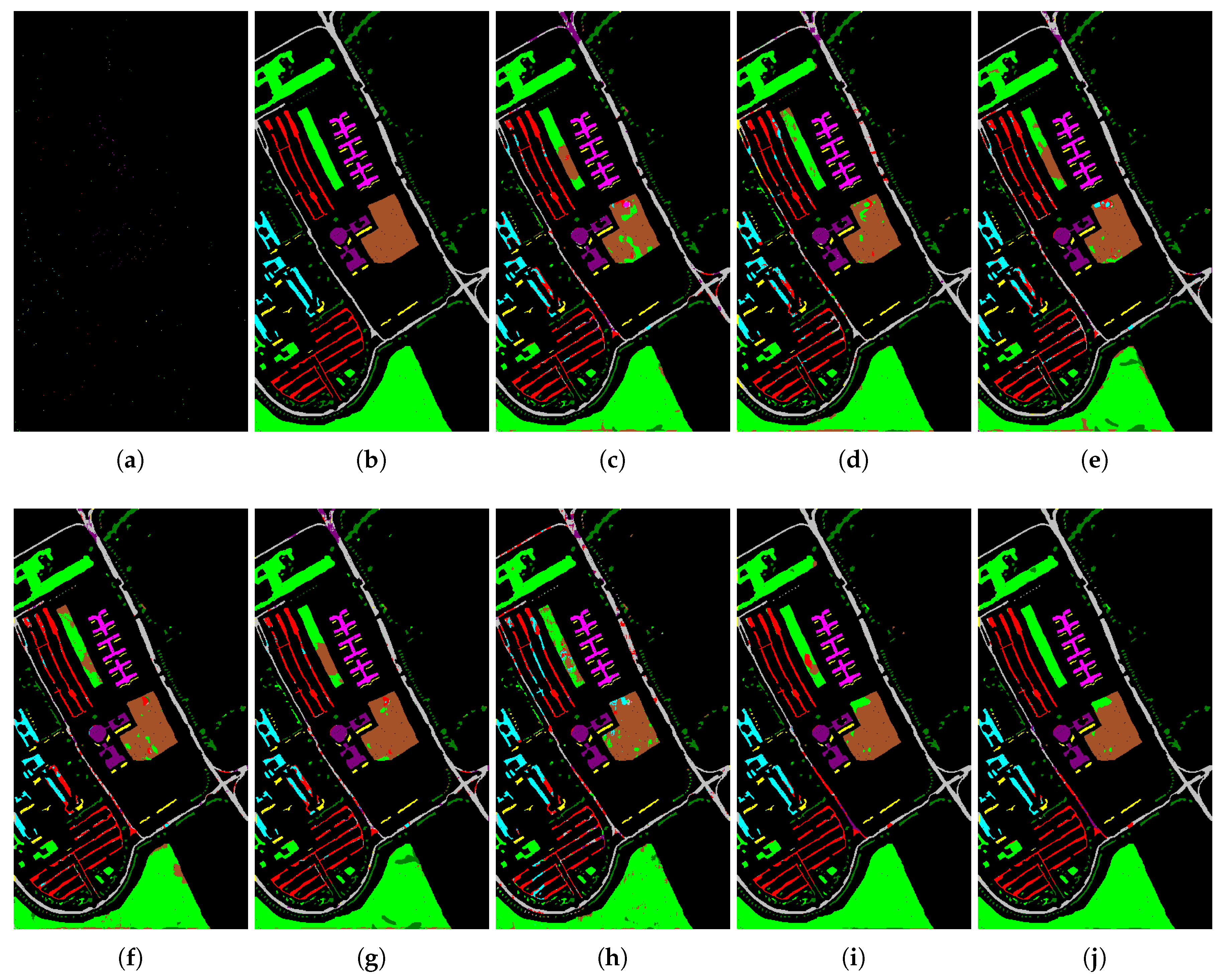
Finally, in order to show the classification results of different methods for each class when limited training data are available, we randomly select 20 samples from each class to compare eight algorithms. The results from different algorithms are objectively and subjectively shown in

Table 3. Classification results of different DR methods based on SVM on the Pavia University data (the TPR and FPR of each class are displayed in the left and right sides of the vertical line, respectively).

Class	Samples		DR Models
	Train	Test	SVM	SPPCA	NWFE	SLGDA	LapCGDA	LGSFA	SaCGDA	LapSaCGDA
1	20	6611	83.6 | 93.9	83.6 | 96.2	89.3 | 92.7	89.3 | 95.1	85.3 | 96.0	80.8 | 92.3	91.6 | 97.1	91.1 | 97.7
2	20	18,629	92.6 | 95.3	95.9 | 96.4	88.6 | 97.9	91.6 | 97.9	90.7 | 97.5	92.9 | 96.3	96.8 | 96.9	98.8 | 97.0
3	20	2079	79.6 | 87.3	78.3 | 83.0	81.0 | 84.5	75.6 | 91.3	79.8 | 91.5	83.5 | 63.3	92.5 | 98.9	93.2 | 98.7
4	20	3044	90.5 | 90.4	85.4 | 94.0	90.6 | 80.0	92.1 | 92.1	88.6 | 77.6	80.3 | 93.5	90.8 | 92.4	90.6 | 91.7
5	20	1325	99.6 | 96.1	100.0 | 99.8	100.0 | 99.6	100.0 | 99.6	100.0 | 99.8	98.4 | 100.0	100.0 | 99.8	100.0 | 99.9
6	20	5009	82.2 | 77.0	93.0 | 86.4	91.0 | 73.9	93.1 | 76.8	94.5 | 81.4	90.3 | 80.7	92.2 | 94.4	92.5 | 99.7
7	20	1310	97.0 | 66.2	98.5 | 83.0	98.3 | 82.8	98.6 | 83.4	98.7 | 71.8	98.1 | 77.3	98.3 | 87.7	98.5 | 84.8
8	20	3662	88.7 | 78.8	86.7 | 76.7	85.2 | 79.4	91.6 | 78.2	91.8 | 80.6	72.9 | 67.0	96.5 | 85.1	96.5 | 89.3
9	20	927	94.6 | 97.2	97.3 | 76.1	94.9 | 93.3	96.2 | 93.3	95.6 | 90.2	95.8 | 94.6	95.9 | 91.5	97.1 | 87.0
AA(%)			86.9	88.0	87.1	89.7	87.4	85.0	93.7	94.0
OA(%)			89.3	91.5	89.3	91.2	90.4	88.0	94.9	95.8
KC			0.9	0.9	0.9	0.9	0.9	0.8	0.9	0.9

and Figure 6, respectively. What can be seen from Table 3 is that the proposed SaCGDA and LapSaCGDA outperform other models in terms of the AA, OA, KC as well as TPR and FPR in most classes, and LapSaCGDA achieves higher accuracy than SaCGDA, which clearly indicates that the Laplacian regularization in LapSaCGDA is beneficial to the DR model. Accordingly, Figure 6 subjectively tells us that classification maps from the proposed methods w.r.t. the testing data are more accurate than other contrastive approaches.

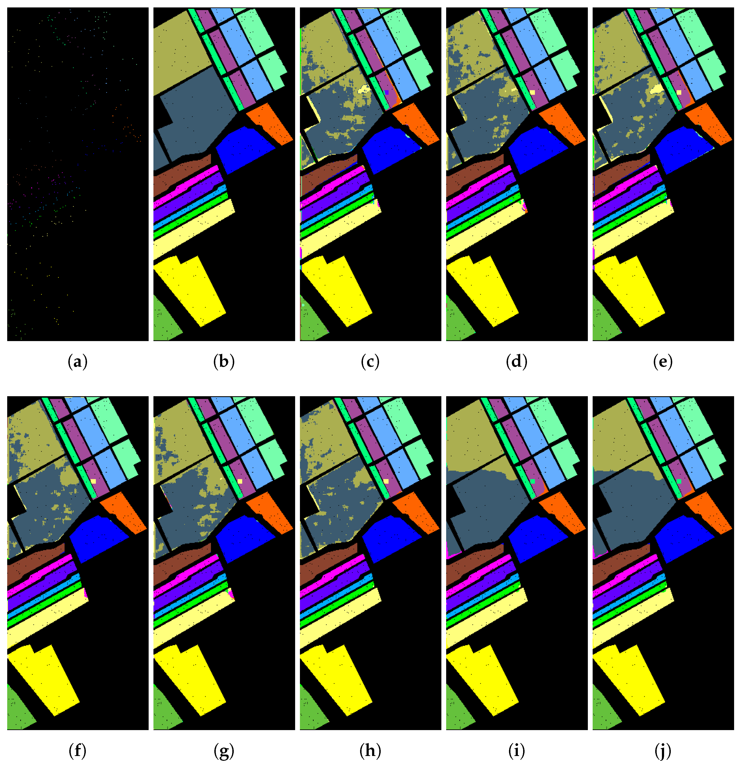
4.3. Experiments on the Salinas Data

To further verify the proposed models on HSIs data from different HSIs sensors, we utilize Salinas data captured by AVIRIS sensor to demonstrate the effectiveness of the novel methods. Similarly, we firstly select the optimal regularization parameters such as $\alpha ,\beta ,\gamma$ in LapCGDA, SLGDA, and, in addition to the regularization parameters, the smooth parameter t in the spatial prior for the proposed SaCGDA and LapSaCGDA by the grid search. The embedding dimensionality is set 30 and 30 training samples are randomly picked from each class so that the parameter sensitivity can be compared.

According to Figure 7a, the regularization parameter $\alpha$ in SaCGDA becomes sensitive to the OA, but the optimal value is still less than 0.001. Thus, we set $\alpha =0.0001$ for both SaCGDA and LapSaCGDA. In addition, it can be viewed from Figure 7b that the optimal parameter $\gamma$ w.r.t. the spectral manifold prior in LapSaCGDA is 0.1, which means that this manifold prior affects the DR model largely compared to the parameter $\alpha$ w.r.t. the spectral locality prior. Additionally, for this dataset, the best smooth parameter t in the spatial prior in SaCGDA and LapSaCGDA is 4 by grid search.

Table 4. Optimal parameters settings for LapCGDA, SLGDA, SaCGDA and LapSaCGDA on the Salinas data.

Model	$\mathit{\alpha }$	$\mathit{\beta }$	$\mathit{\gamma }$
LapCGDA	0.01	1	—
SLGDA	10	10	—
SaCGDA	0.0001	1000	—
LapSaCGDA	0.0001	1000	0.1

displays the best parameters obtained from the parameter sensitivity experiments, which will be used in the following experiments.

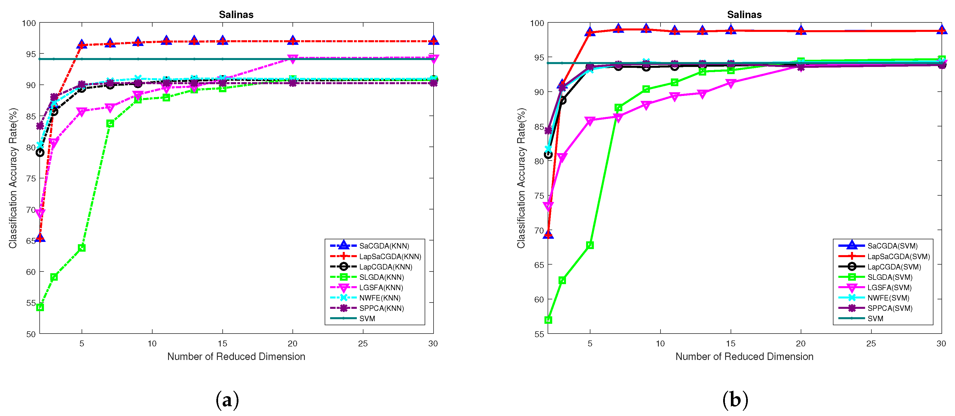
Once these optimal parameters are selected by the grid search, we should choose the best dimensionality of the projection space in terms of the OAs based on KNN and SVM performed in the low-dimensional projection space. What can be seen from Figure 8 is that the proposed SaCGDA and LapSaCGDA outperform other DR models almost in all low-dimensional projection space again, and the optimal number of dimensionality for each DR model in this HSIs data is 30.

Furthermore, based on the optimal projection dimensionality, we also objectively show the experimental results as the amount of training data increases. In addition, 20–80 samples are randomly picked from all the labeled data, and the rest of the samples are for testing. We can conclude from

Table 5. Classification results with different numbers of training data on the Salinas data (OA ± STD (%)).

Classifier	DR Model	${\mathit{n}}_{\mathit{l}}=20$	${\mathit{n}}_{\mathit{l}}=40$	${\mathit{n}}_{\mathit{l}}=60$	${\mathit{n}}_{\mathit{l}}=80$
KNN	SPPCA	89.47 ± 5.9	92.08 ± 3.35	92.74 ± 2.03	94.36 ± 2.13
	NWFE	88.57 ± 1.81	91.08 ± 0.61	92.24 ± 0.58	93.36 ± 0.54
	SLGDA	89.53 ± 1.85	92.7 ± 0.62	93.67 ± 0.71	94.44 ± 0.79
	LapCGDA	88.39 ± 2.25	91.76 ± 1.1	92.71 ± 1.48	93.52 ± 0.78
	LGSFA	92.56 ± 1.53	95.16 ± 0.55	95.76 ± 0.51	96.36 ± 0.32
	SaCGDA	97.34 ± 0.65	98.29 ± 0.43	98.69 ± 0.49	98.93 ± 0.31
	LapSaCGDA	97.29 ± 0.43	98.58 ± 0.34	98.7 ± 0.15	98.92 ± 0.19
SVM	SPPCA	92.92 ± 0.96	95.06 ± 0.53	95.91 ± 0.37	96.47 ± 0.42
	NWFE	92.85 ± 1.01	94.62 ± 0.56	95.31 ± 0.67	96.32 ± 0.26
	SLGDA	92.9 ± 1.25	95.25 ± 0.6	96.02 ± 0.34	96.35 ± 0.41
	LapCGDA	92.66 ± 1.25	94.98 ± 0.87	95.65 ± 0.91	96.58 ± 0.15
	LGSFA	92.46 ± 1.37	95.06 ± 0.56	96.08 ± 0.43	96.85 ± 0.43
	SaCGDA	99.05 ± 0.31	99.44 ± 0.15	99.41 ± 0.35	99.62 ± 0.21
	LapSaCGDA	99.04 ± 0.24	99.38 ± 0.28	99.48 ± 0.11	99.61 ± 0.15

that the proposed SaCGDA and LapSaCGDA achieve the best OAs, especially when only a few pieces of training data are available.

Finally, we select 20 samples from each class to compare all the models in terms of the classification accuracy for each class. As can be viewed from

Table 6. Classification results of different DR methods based on SVM on the Salinas data (the TPR and FPR of each class are displayed in the left and right sides of the vertical line, respectively).

Class	Samples		DR Models
	Train	Test	SVM	SPPCA	NWFE	SLGDA	LapCGDA	LGSFA	SaCGDA	LapSaCGDA
1	20	1989	92.2 | 96.1	100.0 | 99.2	94.0 | 100.0	99.5 | 98.5	99.9 | 100.0	100.0 | 100.0	99.6 | 100.0	99.6 | 100.0
2	20	3706	99.3 | 96.8	99.9 | 100.0	98.8 | 97.0	99.9 | 99.7	99.9 | 100.0	100.0 | 100.0	100.0 | 99.8	100.0 | 99.8
3	20	1956	99.5 | 90.3	99.8 | 98.5	99.8 | 92.6	100.0 | 99.9	100.0 | 99.0	100.0 | 99.3	100.0 | 95.6	100.0 | 94.7
4	20	1374	97.1 | 95.6	96.7 | 99.0	97.3 | 99.3	97.2 | 99.0	98.0 | 98.5	97.7 | 99.8	97.7 | 92.6	98.0 | 91.6
5	20	2658	88.2 | 95.7	97.8 | 97.1	92.0 | 95.7	97.4 | 97.6	97.9 | 98.0	97.3 | 97.7	94.4 | 98.7	93.9 | 99.3
6	20	3939	99.2 | 100.0	99.8 | 100.0	99.5 | 100.0	99.6 | 100.0	99.9 | 100.0	100.0 | 100.0	100.0 | 100.0	100.0 | 100.0
7	20	3559	98.3 | 98.0	99.9 | 99.9	98.7 | 98.6	100.0 | 99.8	99.5 | 99.9	100.0 | 100.0	100.0 | 100.0	99.9 | 100.0
8	20	11,251	71.7 | 86.6	82.7 | 84.6	81.9 | 93.4	83.8 | 87.6	75.7 | 90.8	85.5 | 89.0	91.1 | 95.8	91.9 | 96.1
9	20	6183	99.6 | 99.8	99.9 | 99.6	99.7 | 99.7	99.8 | 99.7	99.9 | 99.8	99.8 | 100.0	100.0 | 99.6	100.0 | 99.5
10	20	3258	96.4 | 82.1	96.3 | 89.0	96.7 | 81.2	98.1 | 91.9	96.9 | 91.9	99.9 | 93.1	98.9 | 99.7	98.6 | 99.6
11	20	1048	95.9 | 93.6	99.9 | 96.7	96.6 | 92.8	100.0 | 96.3	98.8 | 94.3	99.5 | 100.0	98.7 | 89.5	99.6 | 92.1
12	20	1907	97.2 | 95.7	99.0 | 99.6	98.1 | 97.3	99.0 | 99.9	99.7 | 98.8	100.0 | 99.9	99.8 | 99.6	99.7 | 99.7
13	20	896	94.5 | 95.1	98.0 | 98.2	96.0 | 97.9	99.1 | 100.0	97.0 | 99.2	99.9 | 100.0	99.3 | 99.9	99.7 | 100.0
14	20	1050	97.2 | 79.0	99.0 | 92.9	98.8 | 75.5	100.0 | 97.3	99.9 | 96.2	99.5 | 99.0	99.0 | 98.5	99.4 | 98.2
15	20	7248	80.1 | 69.5	74.7 | 75.8	86.8 | 82.1	80.6 | 78.0	85.9 | 70.6	83.2 | 80.4	93.3 | 88.4	93.4 | 89.2
16	20	1787	94.0 | 95.9	97.8 | 100.0	99.3 | 97.5	99.3 | 100.0	99.1 | 96.4	99.2 | 99.8	100.0 | 100.0	100.0 | 100.0
AA(%)			91.9	95.6	93.8	96.6	95.8	97.4	97.4	97.5
OA(%)			89.4	92.3	93.0	93.5	92.5	94.4	96.8	96.9
KC			0.9	0.9	0.9	0.9	0.9	0.9	1.0	1.0

, the proposed two models obtain the highest accuracy in almost every class, and LapSaCGDA is slightly superior to SaCGDA due to the Laplacian prior in LapSaCGDA. The classification maps in Figure 9 give a similar conclusion.

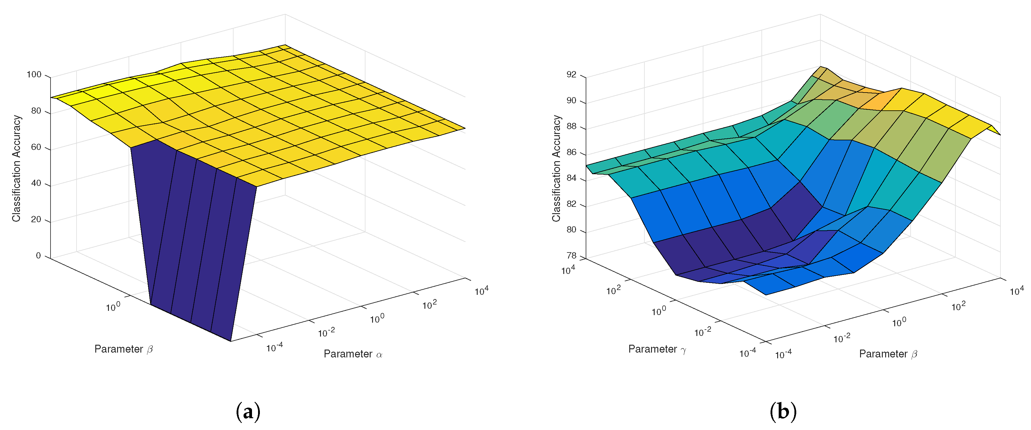
4.4. Experiments on the Indian Pines Data

Another challenging HSIs data is the Indian Pines Data, also captured by the AVIRIS sensor. The optimal regularization parameters such as $\alpha ,\beta ,\gamma$ in the proposed SaCGDA and LapSaCGDA can be observed from the parameters’ sensitivity analysis experiments in Figure 10, and the best smooth parameter t in the spatial prior is 2. Thirty training samples are randomly picked from each class in these experiments, and the projecting dimensionality is also fixed to 30 so that the parameter sensitivity analysis can be demonstrated.

What can be viewed from Figure 10a is that the OAs are not sensitive to the parameter $\alpha$ w.r.t. the spectral locality prior in SaCGDA because the optimal parameter $\beta =5000$ which dominates the model is so large that other constraints are ignored. For the LapSaCGDA, the best parameter $\gamma$ w.r.t. the manifold prior is also small according to Figure 10b. The best regularization parameters for LapCGDA, SLGDA, SaCGDA and LapSaCGDA are listed in

Table 7. Optimal parameters settings for LapCGDA, SLGDA, SaCGDA and LapSaCGDA on the Indian Pines data.

Model	$\mathit{\alpha }$	$\mathit{\beta }$	$\mathit{\gamma }$
LapCGDA	0.01	100	—
SLGDA	100	1	—
SaCGDA	0.0001	5000	—
LapSaCGDA	0.0001	5000	0.0001

for the following experiments.

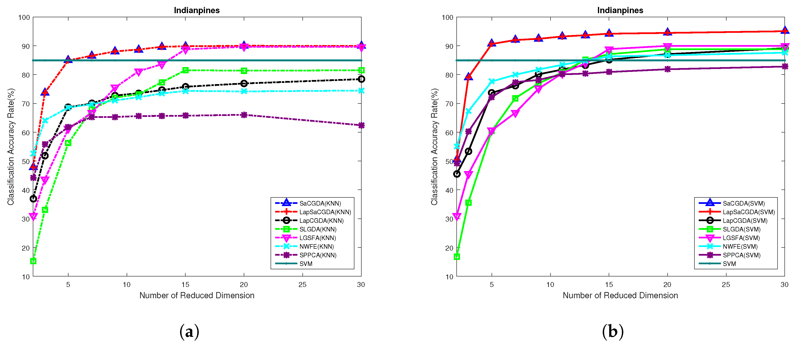
Based on these optimal parameters selected by the grid search, the best dimensionality of the projection space for each DR models can be obtained from Figure 11 in terms of the OAs based on KNN and SVM performed in the low-dimensional projection space. Once again, the optimal number of dimensionality for almost each DR model in this HSI data is 30, and the proposed SaCGDA and LapSaCGDA are the best among all models although LGSFA shows comparative OAs in high-dimensional embedding space based on KNN.

Moreover, we also show the experimental results when different amounts of training data are selected. In addition, 20–80 samples are randomly picked from all the labeled data, and the other samples become the testing data. For those classes where there are less samples available, no more than $60\%$ samples out of all data belonging to some classes will be randomly chosen. It can be seen from

Table 8. Classification results with different amounts of training data on the Indian pines data (OA ± STD (%)).

Classifier	DR Model	${\mathit{n}}_{\mathit{l}}=20$	${\mathit{n}}_{\mathit{l}}=40$	${\mathit{n}}_{\mathit{l}}=60$	${\mathit{n}}_{\mathit{l}}=80$
KNN	SPPCA	66.04 ± 1.42	76.35 ± 1.3	81.18 ± 0.89	84.35±1.05
	NWFE	69.5 ± 1.75	77.93 ± 1.55	81.3 ± 1.06	83.33 ± 1.09
	SLGDA	76.75 ± 1.33	84.59 ± 1.37	88.28 ± 0.98	89.6 ± 1.15
	LapCGDA	67.31 ± 2.68	81.09 ± 1.35	83.9 ± 1.44	85.66 ± 0.85
	LGSFA	84.34 ± 1.62	92.63 ± 1.17	95.15 ± 0.75	95.54 ± 0.85
	SaCGDA	84.97 ± 0.99	91.67 ± 0.5	93.91 ± 0.6	95.45 ± 0.37
	LapSaCGDA	84.97 ± 0.99	91.67 ± 0.49	93.91 ± 0.6	95.45 ± 0.37
SVM	SPPCA	79.26 ± 1.51	85.89 ± 1.12	89.3 ± 0.73	90.92 ± 0.56
	NWFE	83.35 ± 1.49	89.9 ± 0.82	92.37 ± 0.83	93.79 ± 0.9
	SLGDA	85.17 ± 1.39	91.23 ± 0.94	94.17 ± 0.62	95.16 ± 0.99
	LapCGDA	77.18 ± 2.91	91.04 ± 0.9	93.61 ± 0.77	94.66 ± 0.72
	LGSFA	84.05 ± 1.94	92.59 ± 1.15	95.37 ± 0.5	95.74 ± 0.59
	SaCGDA	91.43 ± 0.86	95.36 ± 0.77	96.98 ± 0.54	97.85 ± 0.28
	LapSaCGDA	91.43 ± 0.86	95.36 ± 0.77	96.98 ± 0.54	97.85 ± 0.28

that LGSFA demonstrates comparative OAs based on KNN compared to the proposed SaCGDA and LapSaCGDA while the two novel models outperform LGSFA and other methods in terms of the SVM classification accuracy. As the spatial prior with large regularization parameter $\beta =5000$ dominates LapSaCGDA, LapSaCGDA shows the same results compared to SaCGDA because the two spectral constraints in LapSaCGDA are ignored and LapSaCGDA reduces to SaCGDA in this case.

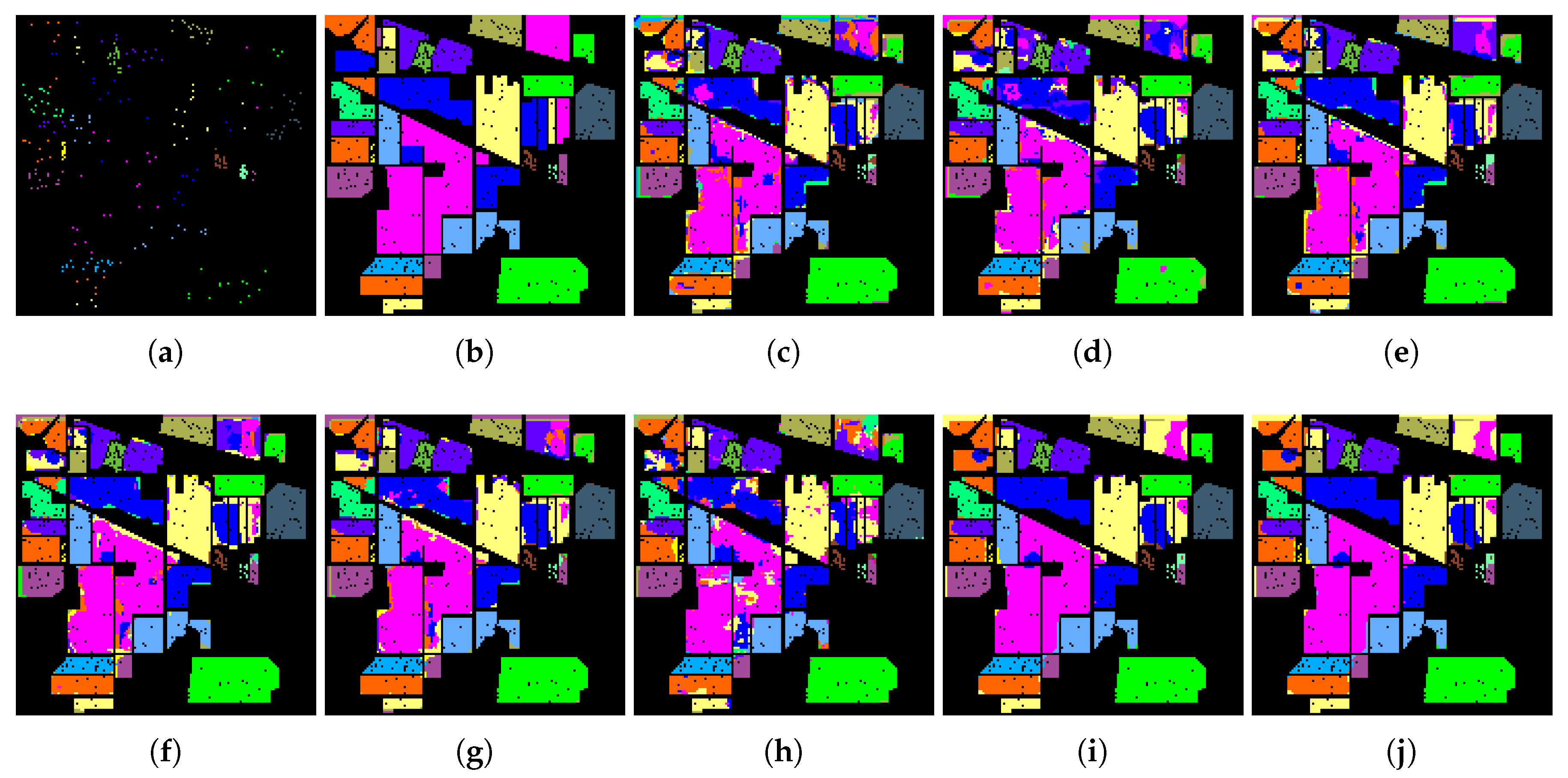
Finally, 20 samples are randomly selected to similarly show the classification accuracy for each class based on SVM. It can be seen from

Table 9. Classification results of different DR methods based on SVM on the Indian pines data (the TPR and FPR of each class are displayed in the left and right sides of the vertical line, respectively).

Class	Samples		DR Models
	Train	Test	SVM	SPPCA	NWFE	SLGDA	LapCGDA	LGSFA	SaCGDA	LapSaCGDA
1	20	26	100.0 | 47.3	100.0 | 43.3	100.0 | 65.0	100.0 | 72.2	100.0 | 59.1	100.0 | 47.3	100.0 | 54.2	100.0 | 54.2
2	20	1408	71.9 | 83.8	63.8 | 77.2	79.0 | 87.4	79.0 | 87.7	75.6 | 92.1	75.5 | 85.3	81.9 | 97.5	81.9 | 97.5
3	20	810	80.5 | 66.1	78.9 | 85.7	82.6 | 86.1	84.6 | 83.2	85.2 | 81.8	80.5 | 73.1	86.7 | 80.8	86.7 | 80.8
4	20	217	96.8 | 73.2	94.5 | 75.9	96.8 | 68.9	95.9 | 73.0	96.3 | 75.5	96.8 | 70.9	98.2 | 95.9	98.2 | 95.9
5	20	463	76.5 | 87.6	76.9 | 100.0	86.4 | 80.8	82.5 | 83.2	86.4 | 72.9	87.3 | 99.5	86.6 | 100.0	86.6 | 100.0
6	20	710	92.4 | 91.4	95.4 | 98.3	96.9 | 94.4	97.0 | 97.5	98.0 | 98.7	94.9 | 90.7	98.0 | 96.4	98.0 | 96.4
7	17	11	100.0 | 30.6	100.0 | 37.9	100.0 | 28.2	100.0 | 78.6	100.0 | 61.1	100.0 | 84.6	100.0 | 33.3	100.0 | 33.3
8	20	458	98.7 | 100.0	99.6 | 100.0	99.6 | 100.0	100.0 | 100.0	99.6 | 100.0	99.6 | 100.0	100.0 | 100.0	100.0 | 100.0
9	12	8	100.0 | 6.5	100.0 | 19.0	100.0 | 8.2	100.0 | 9.9	100.0 | 14.8	100.0 | 26.7	100.0 | 26.7	100.0 | 26.7
10	20	952	82.8 | 71.9	85.4 | 62.0	86.6 | 67.0	91.2 | 69.7	90.8 | 67.9	89.0 | 63.1	96.3 | 62.4	96.3 | 62.4
11	20	2435	67.9 | 92.4	69.7 | 85.1	71.8 | 95.8	71.7 | 96.3	70.4 | 95.1	64.3 | 91.6	83.1 | 97.5	83.1 | 97.5
12	20	573	90.2 | 67.7	82.5 | 52.4	93.4 | 64.0	92.0 | 67.6	94.6 | 64.5	88.0 | 66.9	95.3 | 95.0	95.3 | 95.0
13	20	185	89.2 | 59.8	99.5 | 99.5	97.3 | 92.3	97.8 | 97.8	98.9 | 98.9	100.0 | 98.9	99.5 | 97.9	99.5 | 97.9
14	20	1245	91.8 | 94.5	93.3 | 98.0	92.7 | 99.7	97.8 | 97.6	96.1 | 99.7	96.5 | 98.8	99.4 | 99.7	99.4 | 99.7
15	20	366	77.3 | 62.6	81.1 | 62.9	79.2 | 70.7	92.3 | 73.2	85.2 | 67.7	97.8 | 69.4	89.1 | 93.1	89.1 | 93.1
16	20	73	100.0 | 88.0	100.0 | 97.3	100.0 | 96.1	100.0 | 94.8	100.0 | 94.8	97.3 | 86.6	100.0 | 96.1	100.0 | 96.1
AA(%)			70.2	74.7	75.3	80.1	77.8	78.3	82.9	82.9
OA(%)			80.5	80.2	84.4	85.8	85.0	82.8	90.3	90.3
KC			0.8	0.8	0.8	0.8	0.8	0.8	0.9	0.9

that the proposed SaCGDA and LapSaCGDA are superior to other models when only the spatial prior is utilized, which demonstrates the effectiveness of the spatial prior once again. Accordingly, Figure 12 shows that the classification maps from the proposed SaCGDA and LapSaCGDA are more accurate than other approaches.

4.5. Discussion

Based on above experimental results, we can provide the following discussions,

(i)

The proposed SaCGDA significantly outperforms SVM, SPPCA, NWFE, SLGDA, LapCGDA and LGSFA in terms of OA, AA, KC, TPR and FPR in most scenarios, and accordingly the classification maps based on the new model are smoother and more accurate than results from other supervised DR algorithms. These results clearly demonstrate that the introduced spatial constraint is very efficient to model the spatial relationship between pixels.

(ii)

The Laplacian regularized SaCGDA (LapSaCGDA) could be superior to SaCGDA by further introducing Laplacian constraint into SaCGDA, which makes similar pixels share similar representations. The experimental results verify that LapSaCGDA achieves higher accuracy than SaCGDA in most cases because LapSaCGDA could reveal the intrinsic manifold structures of HSI data more efficiently.

(iii)

It is also worth pointing out that the SVM classifier always provides better classification results than KNN classifiers. However, if we compare the OAs of KNN based on the proposed two models to OAs of SVM based on other DR techniques like NWFE, SLGDA, LapCGDA and LGSFA, what we can find is that the KNN classification results are better than SVM, which further proves that the proposed two algorithms are more effective to extract discriminative low-dimensional features than other contrastive approaches.

5. Conclusions

This paper presents two novel supervised dimensionality reduction models for HSI data, SaCGDA and LapSaCGDA, based on the Graph-Embedding Discriminant Analysis framework. The proposed SaCGDA constructs the intrinsic graph by CR with spatial constraint introduced by JSaCR, and then, in order to consider the complex data manifold structure embedded into the high-dimensional spectral features, Laplacian constraint is further introduced into SaCGDA, leading to the LapSaCGDA with efficient spectral and spatial regularizations. To further improve the performance of DR models, each sample in HSIs is initially preprocessed by spatially averaging its neighboring pixels, which brings the spectral-spatial features before performing DR. Consequently, various experiments demonstrate that the discriminating features for classification can be effectively extracted based on the new models.

For future works, various spatial constraints such as local reconstruction points, superpixel and hypergraph based spatial regularization models in LGSFA [44], SLGDE [29] and SSHGDA [43] can also be introduced into CGDA, and it is also promising to add penalty graphs to the proposed LapSaCGDA, which could further boost the performance.