Potential of Cost-Efficient Single Frequency GNSS Receivers for Water Vapor Monitoring

Abstract

Dual-frequency Global Navigation Satellite Systems (GNSSs) enable the estimation of Zenith Tropospheric Delay (ZTD) which can be converted to Precipitable Water Vapor (PWV). The density of existing GNSS monitoring networks is insufficient to capture small-scale water vapor variations that are especially important for extreme weather forecasting. A densification with geodetic-grade dual-frequency receivers is not economically feasible. Cost-efficient single-frequency receivers offer a possible alternative. This paper studies the feasibility of using low-cost receivers to increase the density of GNSS networks for retrieval of PWV. We processed one year of GNSS data from an IGS station and two co-located single-frequency stations. Additionally, in another experiment, the Radio Frequency (RF) signal from a geodetic-grade dual-frequency antenna was split to a geodetic receiver and two low-cost receivers. To process the single-frequency observations in Precise Point Positioning (PPP) mode, we apply the Satellite-specific Epoch-differenced Ionospheric Delay (SEID) model using two different reference network configurations of 50–80 km and 200–300 km mean station distances, respectively. Our research setup can distinguish between the antenna, ionospheric interpolation, and software-related impacts on the quality of PWV retrievals. The study shows that single-frequency GNSS receivers can achieve a quality similar to that of geodetic receivers in terms of RMSE for ZTD estimations. We demonstrate that modeling of the ionosphere and the antenna type are the main sources influencing the ZTD precision.

1. Introduction

Water vapor plays an important role for atmospheric processes. It is the most abundant greenhouse gas [1] and is spatially and temporally highly variable [2]. Atmospheric water vapor is essential for convection in the lower atmosphere and hence crucial for the generation of clouds and rainfall. A relationship between water vapor fields and severe weather events has been observed, e.g., by Seko et al. [3]. With regard to a warming climate, the amount of water vapor in the atmosphere increases and causes additional absorption of long-wave radiation and reflects it back to the ground [4]. Water vapor also transports latent heat through the atmosphere. Distribution of atmospheric water vapor is an important factor for weather models, and its monitoring is crucial for weather research. The traditional method to measure water vapor in the air is by releasing radiosonde balloons. However, the releases are typically only performed a few times per week and are characterized by distances often greater than 100 km.

Another approach is to determine Precipitable Water Vapor (PWV) from the observed delay in Global Navigation Satellite System (GNSS) transmitted signals. The estimated Zenith Tropospheric Delay (ZTD) is the driving factor to obtain PWV, and uncertainties in ZTD dominate the error budget of PWV [5]. Monitoring local inhomogeneities of water vapor that may be associated with deep convection is important for the prediction of severe weather events. One should note that existing weather radars can only detect clouds after the start of precipitation. Currently, PWV derived from globally, nationally, and regionally distributed networks of dual-frequency receivers is used to improve existing numerical weather models [6]. The networks were originally designed for geodetic applications and are characterized by an inhomogeneous distribution and inter-station distances in the order of tens of kilometers or above. Due to their high inter-station distances, these networks are often not sufficiently dense to monitor small-scale water vapor fluctuations ([7,8]). Real-Time Kinematic (RTK) networks are already characterized by station distances below 30 km (e.g., Netherlands or Germany). Some networks, such as the Japanese GEONET, even reach inter-station distances of about 20 km [9]. In our study, networks with average station distances of around 30 km are considered as dense. Regional networks in Europe with station distances between 70 and 100 km are considered as low-density networks. However, even networks with inter-station distances of 20 km are not dense enough to properly detect water vapor variations associated with localized convective phenomena [10]. The cost of dual-frequency receivers exceeds several thousands dollars. Driven by these economic reasons, the use of dual-frequency receivers for water vapor monitoring is not feasible at high density. Instead, inexpensive single-frequency receivers already available at a cost of a hundred to a few hundred dollars offer an interesting alternative. Having been designed to be embedded into mass-market devices such as car navigation equipment and smartphones, these inexpensive receiver modules and antennas are more economical than their dual-frequency geodetic counterparts in terms of both money and power consumption (in case of off-grid application).

Currently, widespread application of single-frequency GNSS is limited by errors introduced by the ionosphere. Different strategies exist to obtain ZTD estimations, e.g., the network approach based on double differences or the Precise Point Positioning (PPP) based on undifferenced observations. A comprehensive analysis using different mapping functions, cutoff angles, and positioning methods has been performed by Baldysz et al. [11]. In that study, the PPP performed better than the differential approach for PWV linear trend analysis. To account for the error caused by the ionosphere, we apply the Satellite-specific and Epoch-differenced Ionospheric Delay (SEID) model as proposed by Deng et al. [12]. This allows us to treat the single-frequency data as dual-frequency data and process it with well known PPP software [13]. The primary goal of this study is to investigate the feasibility of low-cost single-frequency receivers to densify existing dual-frequency networks and examine the error sources that the receivers are prone to. The research is a first step to examine the potential wide-spread deployment of low-cost GNSS receivers in data sparse regions with limited investment budgets. It aims to highlight the trade-off between using cost-efficient devices compared to their expensive, geodetic-grade dual-frequency counterparts for water vapor monitoring. For this purpose, we conducted a monitoring experiment alongside an International GNSS Service (IGS) station and compared our results with available reference datasets. Earlier studies, e.g., by Deng et al. [12], Deng et al. [14], and Realini et al. [8] demonstrated the feasibility of applying single-frequency GNSS in PPP mode. In our study, we used two different types of low-cost on-site single-frequency receivers and investigated their performance for monitoring water vapor. Durable, weather-proof stations incorporating low-cost GNSS receivers are a recent development and were not available on the market before 2015. Even today only a few startup and small- and medium-sized enterprises produce them. One of the low-cost single-frequency stations used in this study is the GeoGuard Monitoring Unit (GMU) designed by the Italian company GReD [15]. All components are Ingress Protection (IP) 66 or 67 certified and the first units operate since November 2015. Currently 70 GMU stations are continuously monitored by GeoGuard from which some are also deployed in harsh conditions, such as mountainous areas above 2000 m and near the sea. Even though our experimental setup could make use of an already dense RTK network for the ionospheric interpolation, we selected more challenging station distances and only a minimum of SEID reference stations. The study uses exclusively open-source models and publicly available datasets to support the applicability of the setup to other locations. By co-locating multiple different sensors and splitting the antenna signal of a calibrated geodetic-grade antenna to a geodetic-grade receiver, low-cost single- and dual-frequency devices, we were able to make statements about the impact of receiver-and antenna-related errors. The study is organized as follows: Section 2 describes the basics of the GNSS meteorology, the SEID algorithm, and the experimental setup and data processing methods. Section 3 illustrates the ZTD reference comparison, the experimental setup results using two different SEID constellations, and the split antenna experiment results. Section 4 and Section 5 contain the discussion and conclusions, respectively.

2. Methodology

2.1. Water Vapor from GNSS Measurements

Traditional GNSS geodesy aims to obtain precise positioning information from the signal delay between a GNSS receiver and satellites in sight. The delay is affected by several error sources such as clock errors, antenna phase center variations, and tropospheric and ionospheric delays. The tropospheric delay is further separated into a dry (hydrostatic) delay and a wet delay as a result of atmospheric water vapor. The Slant Total Delays (STDs) along each satellite-receiver line of sight are mapped to the zenith direction in order to estimate the ZTD. In GNSS meteorology, the ZTD can be directly assimilated in numerical weather models, or the ZTD can be converted into PWV using surface pressure data and a simple model of the atmosphere.

According to Thayer [16], the refractivity in the troposphere can be considered as the sum of a dry (hydrostatic) and wet component, which can be related to the atmospheric temperature and partial pressure of water vapor and dry gases:

$$N=N_{dry}+N_{wet}=k_1\frac{p_d}{T}+k_2\frac{e}{T}+k_3\frac{e}{T^2}$$

(1)

where $k_1\frac{p_d}{T}$ accounts for the dry part and the last two terms for the wet part. $p_d$ is the combined partial pressure of dry gases in mbar, T the temperature in degree Kelvin, and e the partial pressure of water vapor in mbar. The empirical constants $k_1=(77.604\pm 0.014)K$ mbar${}^{-1}$, $k_2=(64.79\pm 0.08)K$ mbar${}^{-1}$ and $k_3=(3.776\pm 0.004){10}^5{K}^2$ mbar${}^{-1}$ were determined by Thayer [16]. The integrals of the refractivity N in the zenith direction are referred to as Zenith Hydrostatic Delay (ZHD) and Zenith Wet Delay (ZWD). The ZHD can be estimated using the Saastamoinen model [17]:

$$\mathrm{ZHD}=\frac{0.0022768P_0}{1-0.00266cos\left(2\mathrm{\Phi }\right)-0.00028H}$$

(2)

where $P_0$ is the total atmospheric pressure in mbar expected to be observed at the receiver position, $\mathrm{\Phi }$ is the latitude in radians and H the orthometric height (i.e., above the reference geoid) in kilometers.

Since the wet delay is much more variable than the hydrostatic delay and its predictive value is poor in comparison to the ZHD estimation, the difference between the ZTD and the modeled ZHD is used to obtain the ZWD. The authors of Bevis et al. [18] demonstrate how the ZTD observed from GPS measurements can be used to derive PWV with given pressure and temperature data. Using the ZWD, the PWV can be estimated with a non-dimensional ratio $\mathrm{\Pi }$:

$$\mathrm{\Pi }=\frac{{10}^6}{\rho R_v[\left(\frac{k_3}{T_m}\right)+k_2^{\prime }]}$$

(3)

with $T_m$ being the weighted mean temperature of the atmosphere in degree Kelvin, $\rho$ the density of liquid water in kg m${}^{-3}$, $R_v$ the specific gas constant of water vapor in J (kg K)${}^{-1}$, and $k_2^{\prime }$ defined as $k_2^{\prime }=k_2-m{k}_1$ with m being the ratio of molar masses of water vapor (18.015 g mol ${}^{-1}$) and dry air (28.964 g mol${}^{-1}$). The constants $k_1$, $k_2$, and $k_3$ are the same as proposed by Thayer [16]. The weighted mean temperature of the atmosphere $T_m$ is computed based on radiosonde measurements. However, a simplified model using surface temperature measurements is sufficiently accurate. In our analysis, we use the $T_m$ derived by Baltink et al. [19] based on 9129 radiosonde ascents in De Bilt, The Netherlands:

$$\begin{array}{c}\hfill T_m=0.673T_s+83.0\end{array}$$

(4)

with $T_s$ defined as the surface temperature in Kelvin. The water vapor conversion factor $\mathrm{\Pi }$ ranges typically around 0.16 and varies up to 20% depending on the location, height, and meteorological conditions [20]. The PWV is related to the Integrated Water Vapor (IWV) overlying the receiver, whereby the PWV is defined as the height of an equivalent column of liquid water. The PWV is obtained by

$$\mathrm{PWV}=\mathrm{\Pi }·\mathrm{ZWD}.$$

(5)

Since there are no on-site temperature and air pressure observations available at our experimental setup, we are using measurements from the nearest weather station at a 5 km distance and with a negligible elevation difference. We utilize the EGM2008 geoid model [21] to convert between the ellipsoidal and orthometric height at the station position. The conversion between mean-sea-level atmospheric pressure to the station height is performed by applying a standard lapse rate formula in mbar per meter after the ideal gas law [22]:

$$\frac{\delta P}{\delta h}=-\frac{PMg}{R(T+273.2)}$$

(6)

with P being the pressure in mbar, T the temperature in degree Celsius, M the mean molar mass of atmospheric gases (0.02896 kg mol${}^{-1}$), g the gravity acceleration (9.807 m s${}^{-2}$), and R the universal gas constant (8.314 J K${}^{-1}$ mol${}^{-1}$), respectively. With P being the pressure in mbar and T the temperature in degree Celsius. Accounting for the geoidal undulation is important since the height error will develop a pressure offset. Utilizing the Saastamoinen formula (Equation (2)) shows that a pressure error of one mbar results in an error of around 2.28 mm in ZHD at our station coordinates.

2.2. SEID Ionospheric Delay Modeling

Since it is not possible to obtain an ionosphere-free linear combination of sufficient accuracy based on single-frequency receiver data, the ionosphere must be modeled. In order to process single-frequency receivers within a network of dual-frequency receivers with conventional GNSS processing engines, the authors of Deng et al. [12] developed the SEID model. They use the geometry-free ionospheric observation $L_4$ [23], which is defined as

$$L_4=L_1-L_2={\lambda }_1{A}_1-{\lambda }_2{A}_2-40.28(\frac{1}{f_1^2}-\frac{1}{f_2^2})·STEC(\lambda ,\theta ).$$

(7)

For simplicity the noise and multipath errors are ignored in the equation. $L_1$ and $L_2$ denote the carrier-phase measurements. The term $40.28(\frac{1}{f_1^2}-\frac{1}{f_2^2})·STEC(\lambda ,\theta )$ denotes the ionospheric delay on the system-dependent frequencies $f_1$ and $f_2$. $STEC$ is the Slant Total Electron Content, which is defined as the integral of the electron density along the signal path. $\lambda$ and $\theta$ are latitude and longitude of the Ionospheric Pierce Points (IPPs) of the ray paths on the single-shell defined ionosphere layer at a 350 km height. ${\lambda }_1$ and ${\lambda }_2$ are the wavelengths and $A_1$ and $A_2$ denote the phase ambiguities on the respective frequencies. Ref. [24] demonstrate that the epoch-differenced ionospheric delays are sufficiently accurate to remove the ionospheric delay under normal ionospheric conditions for ZTD estimations. Since the estimation of the ambiguity parameter remains a major obstacle in GNSS processing, the epoch-differences $d{L}_4$ are used:

$$d{L}_4(j+1)=L_4(j+1)-L_4\left(j\right)=40.28(\frac{1}{f_1^2}-\frac{1}{f_2^2})·dSTEC(\lambda ,\theta ).$$

(8)

Utilizing this equation, the ambiguity parameters between two continuously tracked epochs is eliminated. One should note that cycle slips must be removed and phase center variations applied in advance. In small-scale networks, the $dSTEC$ can be modeled with a linear function with the latitude and longitude $\theta$ and $\lambda$ of the IPPs. Each pair of epochs and each satellite can be approximated by the linear function

$$d{L}_4(j+1)=a_0+a_1\lambda +a_2\theta$$

(9)

where the model parameters $a_0$, $a_1$, and $a_2$ are to be estimated by means of least-squares from the epoch-differenced ionospheric delays of the surrounding dual-frequency stations. Using this model, the epoch-differenced ionospheric correction $d{\tilde{L}}_4(j+1)$ of any receiver within the spanned network may be calculated. The sum of the continuously tracked ionospheric corrections from $j_0$ to $j_n$ results in

$${\tilde{L}}_4\left(j_n\right)=\sum _{j_0}^{j_n}d{\tilde{L}}_4+L_4\left(j_0\right).$$

(10)

As depicted in Equation (10), the ionospheric delay at epoch $j_0$ is unknown (thus set to zero). Unfortunately, this destroys the integer nature of the phase ambiguity in the interpolated data, meaning it can never be fixed to integer. However, since in typical PPP, the ambiguities are not fixed to integer (but estimated as float values), this has no impact on the data processing. The synthesized ${\tilde{L}}_2$ signal is constructed from the difference between $L_1$ and ${\tilde{L}}_4$:

$${\tilde{L}}_2=L_1-{\tilde{L}}_4.$$

(11)

The synthesized observable provides the same information as $L_1$, except that the ionospheric delay is adjusted to the $L_2$ frequency. Employing the generated dual-frequency data allows the data to be processed in PPP-mode in conventional PPP analysis tools.

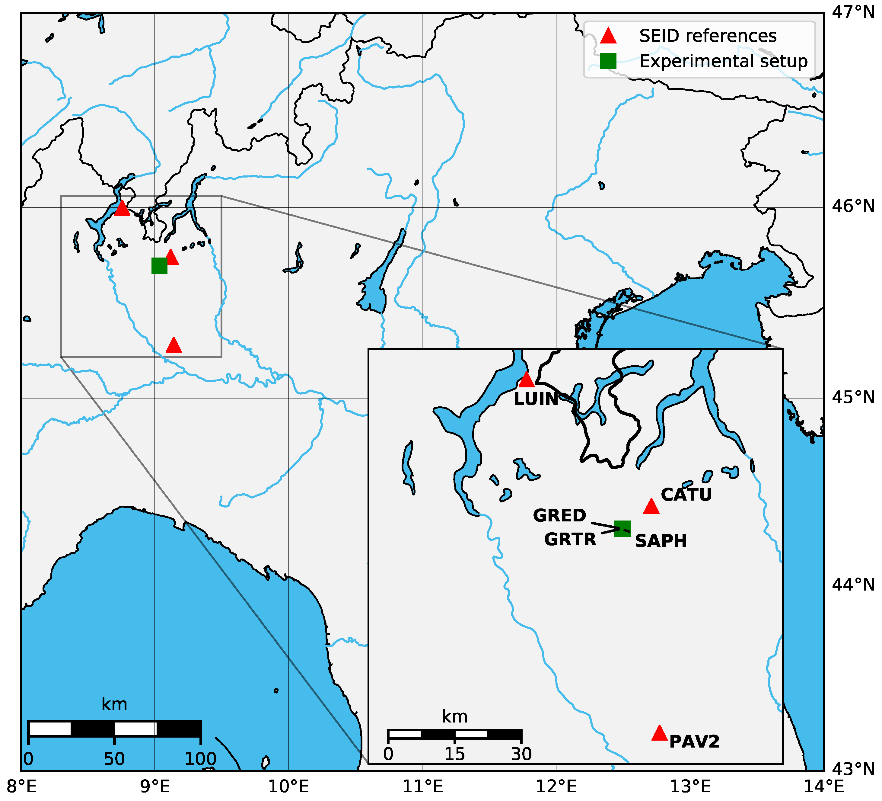
2.3. Experimental Setup and Data Processing

The GNSS data server at the TU Delft collects data from the Dutch Permanent GNSS Array (DPGA), which consists of up to 18 continuously operating dual-frequency receivers throughout the Netherlands. The regional network density is considered as low since its stations are typically located at a 50–100 km distance. The data is publicly available and mainly used for research and educational purposes and providing data to the International GNSS Service (IGS), EUREF Permanent Network (EPN), and EUMETNET GNSS water vapour programme (E-GVAP).

To investigate the feasibility of low-cost single-frequency receivers for water vapor monitoring, we designed an experimental setup along the existing IGS station DLF1 in Delft, The Netherlands. The setup consists of one dual-frequency receiver (IGS station DLF1) and two co-located low-cost single-frequency receivers. The IGS station DLF1 is equipped with a geodetic-grade calibrated choke ring antenna. The antenna type is the current state-of-the-art and serves in our experiment as a reference for the best available antenna observations. One single-frequency station is the GMU which consists of a u-blox LEA-M8T single-frequency receiver with a Tallysman TW3470 antenna. The device has been successfully validated and is currently used for operational deformation monitoring [15]. It is fully autonomous and equipped with a solar panel and wireless (3G) data communication. Additionally, we co-located a u-blox NEO-M8T evaluation toolkit (UBX) equipped with its standard ANN-MS patch antenna.

To apply the SEID algorithm, we selected two SEID reference constellations. The first constellation (DPGA case) consists of 4 stations (VLIS, IJMU, KOS1, and APEL) from the Dutch permanent network. The stations KOS1 and APEL were chosen as a backup for each other, since both have data gaps during the observation period. These are, however, different dates and the SEID model is still functioning by using only 3 instead of 4 reference stations. The total area covered in this case is about 6400 km${}^2$. To analyze the effect of the SEID reference network distances, we added a second SEID constellation (EUREF case) utilizing stations from the EUREF network to our study. The stations are HERT (Great Britain), BORJ (Germany), and DOUR (Belgium). They are located approximately 305, 240, and 215 km from the experimental setup in Delft. The conversion from ZTD to PWV was performed by using data from an Automatic Weather Station (AWS) located 5 km from Delft, operated by the Royal Netherlands Meteorological Institute (KNMI) for temperature and air pressure observations. The station locations are illustrated in Figure 1.

We selected the analysis period from 1 January until 31 December 2017 to cover both low (winter) and high (summer) water vapor activities. During winter, the PWV at this location typically ranges between 1 and 30 mm, whereas the summer is characterized with PWV values between 10 and 50 mm. However, the single-frequency units GMU and UBX have only provided data since September 2017. The IGS station DLF1 provides continuous high-rate data throughout the year with a temporal resolution of up to 1 s. For our analysis, we use this dual-frequency data to perform PPP to obtain a reference ZTD dataset. In order to validate the SEID modeling, we simulate a single-frequency unit (DLF1_SF) by removing the code and phase data from the second frequency (C2 and L2) with the teqc [25] software. Consequently, DLF1 in dual-frequency (DLF1_DF) and synthesized single-frequency mode (DLF1_SF) provide data throughout the year. For all sites (including the SEID network stations), we use 30-second data in the Receiver Independent Exchange Format (RINEX).

The SEID processing and subsequent PPP processing are performed by using the open-source MATLAB program goGPS version 0.4.3 [26]. This version is based on a forward Kalman filter approach. During the pre-processing step, cycle slips are corrected and antenna calibrations, if available, are applied to all stations. An epoch-by-epoch code-only least-squares adjustment is then executed to identify and remove outliers. Observation sets (i.e., code and phase observations for a given satellite) for which the configured residual code observation error threshold is exceeded, are flagged as outliers and removed. Entire epochs are removed if the number of available observation sets is equal or lower than 4, or if the standard deviation of the estimated error exceeds a given threshold. During the PPP processing, an additional outlier detection and removal algorithm is executed, based on a configured threshold on phase post-fit residuals. In this version of goGPS, the PPP Kalman filter is not reset at the day-boundary. This enables a seamless ZTD estimation without spikes at the beginning of each dataset. Both SEID constellation studies and the PPP estimations share the same configuration parameters.

Table 1. SEID and ZTD Computation Settings.

Item	Processing Strategies
Software	goGPS v. 0.4.3
Observations	GPS-only
Sampling interval	30-second
Processing mode	SEID-PPP
Antenna calibration	IGS (if available)
Troposphere modeling	Saastamoinen (with GPT model)
Troposphere mapping function	GMF
Elevation cutoff	10${}^{\circ }$
Ocean loading	FES2004
Observation weighting	same weight for all observations
Clock & orbits	IGS Final
Kalman filter reset	no (seamless)
Code observation error threshold	30 m
Phase observation error threshold	0.05 m
Code least-squares estimation error st. dev. threshold	40 m

summarizes the settings of our analysis.

After the SEID interpolation on the single-frequency datasets, we obtain dual-frequency RINEX files which we process in PPP mode in goGPS. We use data from GPS-only satellites, an elevation cutoff angle of 10 degrees and apply ocean loading effects obtained from the FES2004 model [27]. The IGS antenna calibration, final orbits, 30-second satellite clocks, and earth rotation products are used [28]. One should note that the IGS final products are only available with a 12–18 day latency. Hence, they can only be used for post-processing purposes.

The ZTD estimations are affected by the antenna type and the SEID model. The best possible references for these are calibrated choke ring antennas and dual-frequency PPP estimations. To verify the performance of the goGPS PPP engine, the ZTD estimations are compared to existing reference datasets, respectively. The experimental setup provides these references and allows us to validate these aspects.

A first step in our analysis is the comparison of various available ZTD reference datasets from different analysis centers to results obtained for our experimental setup. Specifically, we compare the reference ZTD data from the IGS available from the Crustal Dynamics Data Information System (CDDIS) archive (IGS [29]), the Nevada Geodetic Laboratory (NGL [30]), and the EPN analysis center outputs [31] from the Federal Agency for Cartography and Geodesy (BKG), Federal Office of Topography (LPT), and the Royal Observatory of Belgium (ROB).

3. Results

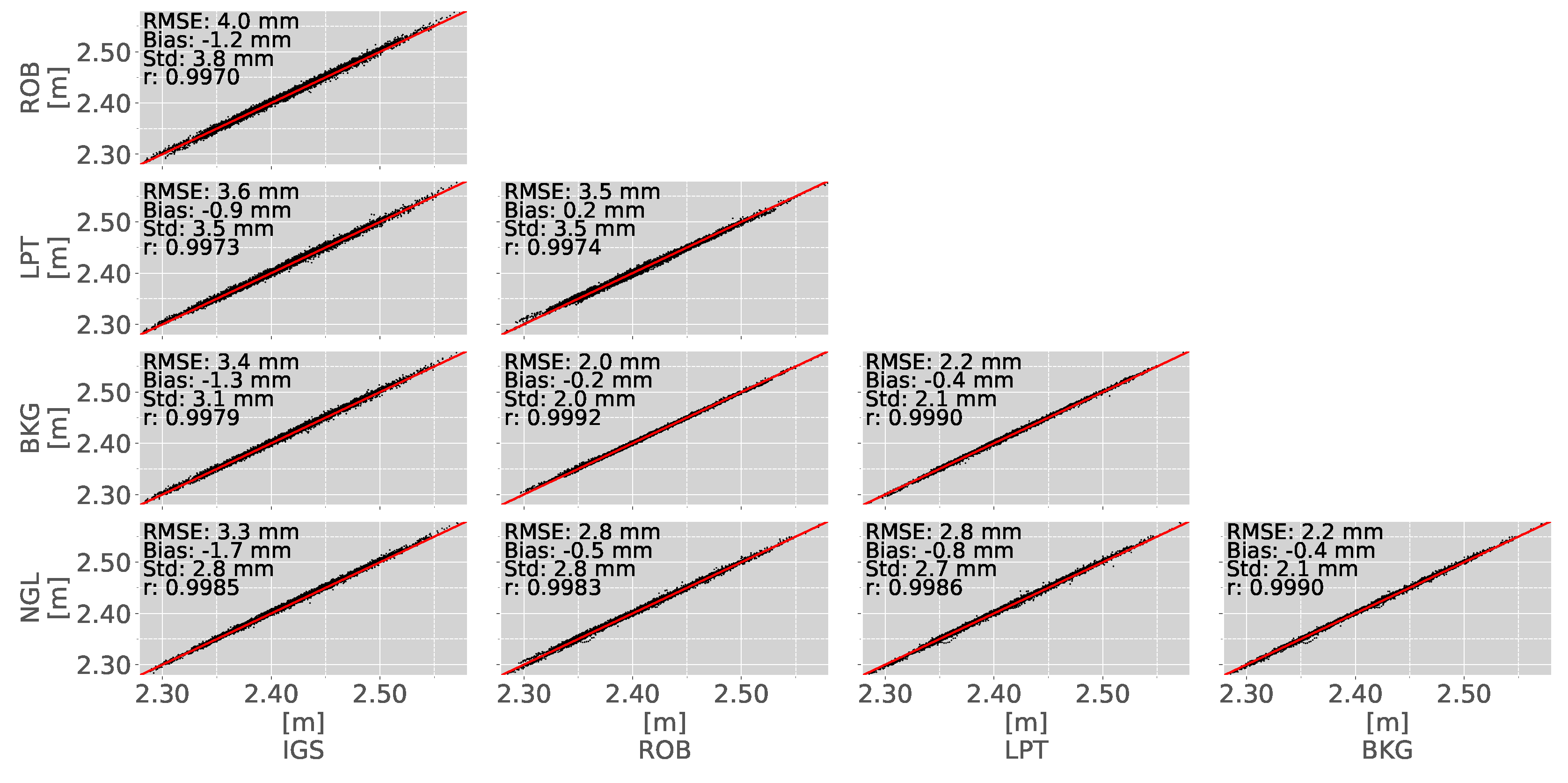
3.1. Inter-Comparison of Different ZTD Reference Datasets

Analysis Centers (ACs) provide ZTD estimations for IGS stations worldwide. However, only the IGS and NGL datasets have a 5 min temporal resolution. The EPN products ROB, LPT, and BKG are available in 1 h intervals. The reference datasets IGS, BKG, LPT, and ROB are based on the Bernese processing engine using the least-squares adjustment method. NGL provides GIPSY/OASIS II ZTD estimations in PPP using a modified Kalman filter. The IGS data is available from the CDDIS archive. The IGS AC updated their processing engine on DOY 29 in 2017 to Bernese 5.2.

Table 2. Characteristics of reference datasets of the IGS station DLF1. All products are post-processed results using the final satellite orbit and clock data.

AC	Processing Engine	Processing Method	Cutoff (${}^{\circ }$)	Resolution	Missing Days
IGS	Bernese 5.0 & 5.2	PPP	7	5 min	10
NGL	GIPSY/OASIS II	PPP	7	5 min	10
BKG	Bernese 5.2	Double-Differences	3	60 min	1
LPT	Bernese 5.3	Double-Differences	3	60 min	4
ROB	Bernese 5.2	Double-Differences	3	60 min	4

summarizes the characteristics of each reference dataset.

Surprisingly not all analysis centers provide data for all dates, whereas the IGS station DLF1 recorded data throughout the selected observation period. As a result, our PPP-processed dual- and simulated single-frequency data of DLF1 is characterized by no data gaps. The IGS and NGL datasets show 10 missing days, whilst BKG, LPT, and ROB show only 1 and 4, respectively. It must be noted that these are for the most part not the same dates. We assess the performance of the ZTD estimations by comparing the various reference datasets to each other. The scatter plots of all reference datasets, their corresponding root mean square errors (RMSE), mean biases and standard deviations are depicted in Figure 2.

The scatter plots show an RMSE of about 3 mm between the post-processed datasets IGS, NGL, BKG, LPT, and ROB. No remarkable bias is observed. The best agreement is found between the 1 h datasets BKG, ROB, and LPT. This is explained by the fact that for the 1 h datasets individual estimates are based on more measurements compared to the 5 min datasets and by the fact that the three ACs use a similar processing method. For the comparison with IGS and NGL, we use the timestamps of the 1 h datasets. The precision of the ZTD estimations between the analysis center outputs are very similar, in the order of 2–4 mm. For this reason, we only use the IGS data as a reference to compare the results from our experimental setup. The advantage of the IGS estimations is the 5 min sampling interval and the high data availability.

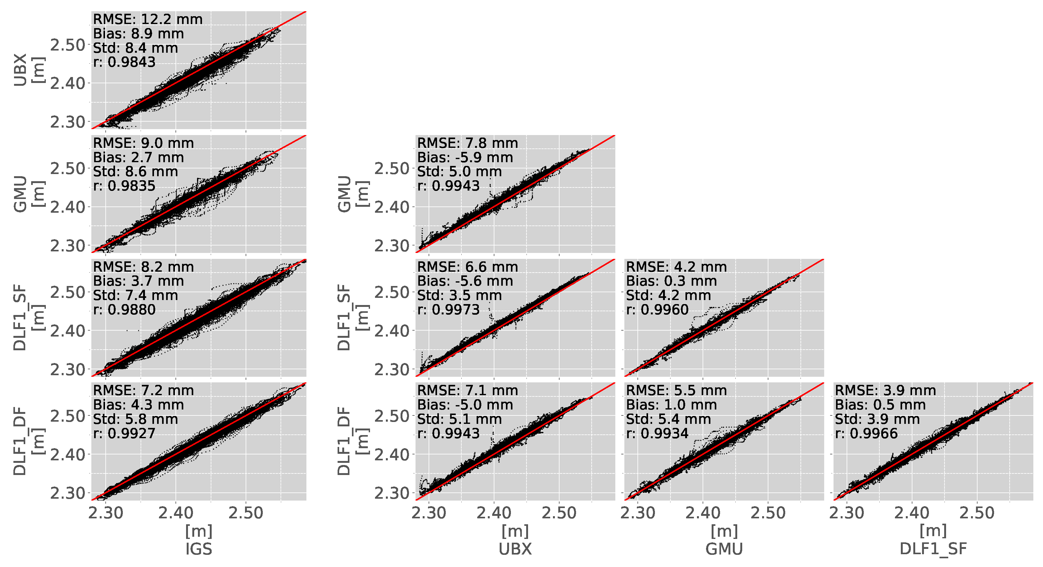
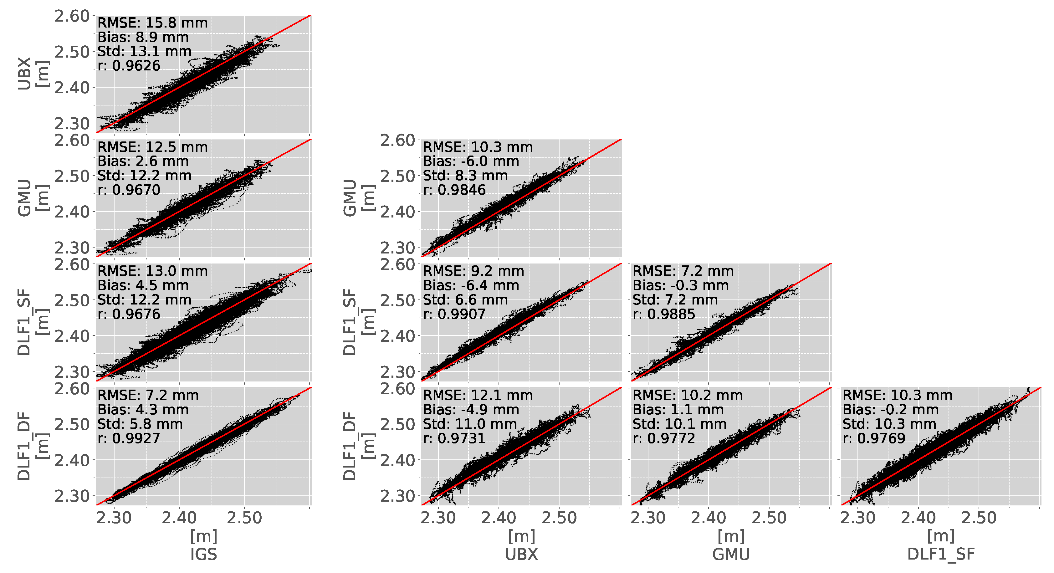
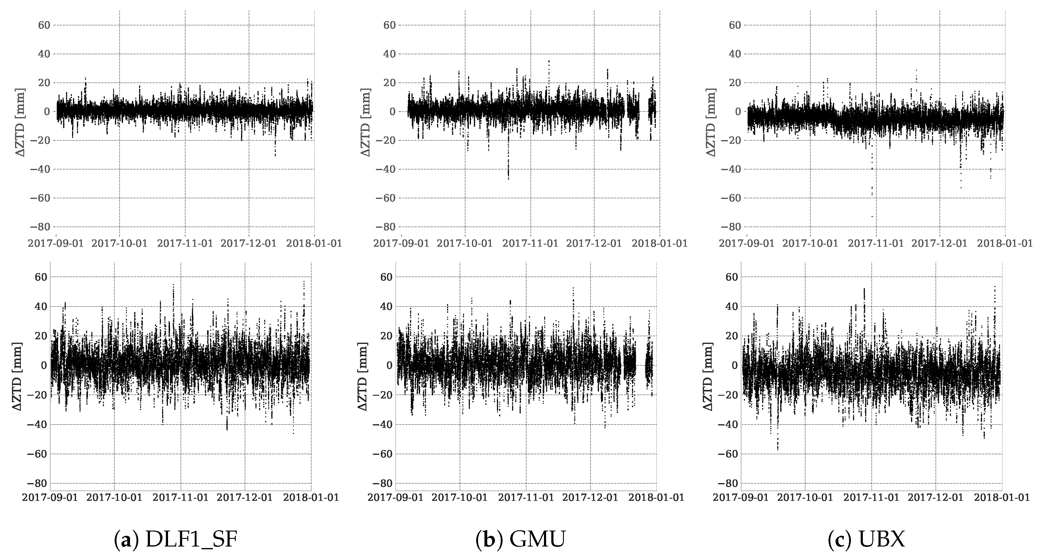
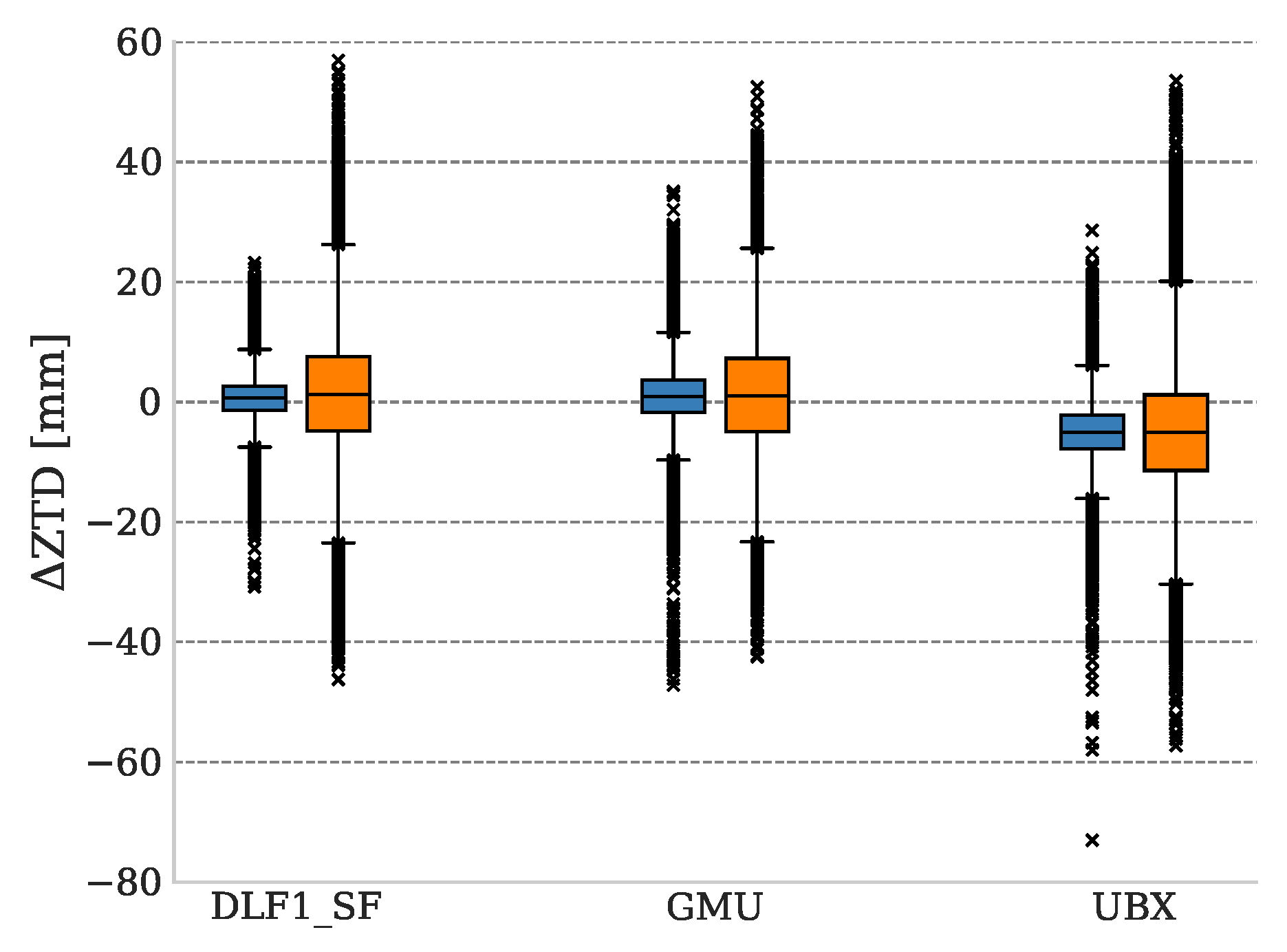
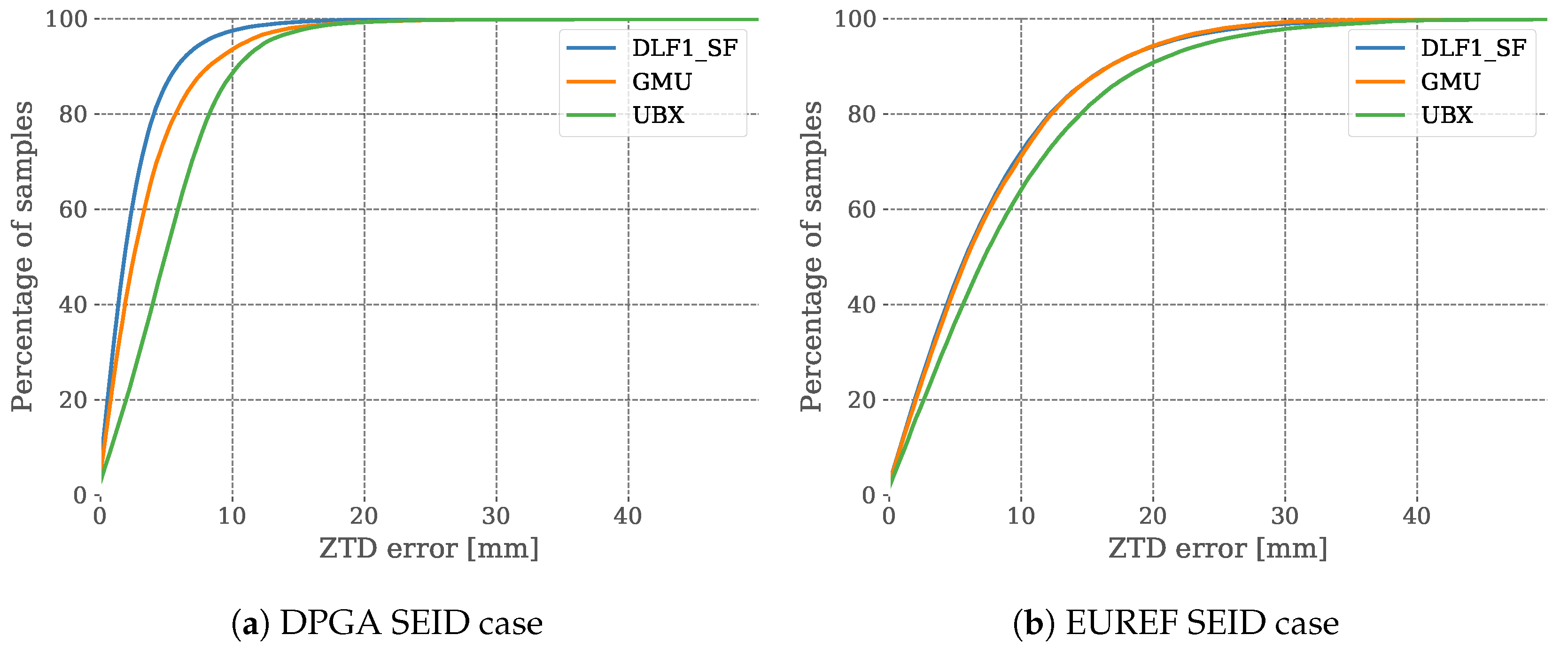
3.2. SEID-PPP-Processed ZTD Estimations

After validating the reference data, we analyzed the results of the goGPS PPP estimations at the experimental setup location for both SEID constellations. Figure 3 shows the ZTD scatter plots between the DLF1 dual- (DLF1_DF) and single-frequency (DLF1_SF), GMU, UBX, and the selected IGS reference dataset using the DPGA SEID constellation.

The column on the left in Figure 3 demonstrates the goGPS PPP software error by comparing the estimations to the IGS reference ZTD dataset. Compared to the IGS reference dataset, the goGPS PPP dual-frequency dataset (DLF1_DF) shows an RMSE of 7 mm and a bias of 4 mm over the whole year. A bias in the range of 3–9 mm is present in the goGPS-processed results and negatively influences the RMSE. The scatter plots on the right show the comparisons of the goGPS estimated results among each other. The dual-frequency data (DLF1_DF) and the simulated SEID-processed single-frequency data (DLF1_SF) show an RMSE of 4 mm. The GMU yields an RMSE of 6 mm and no notable bias. The UBX dataset is largely characterized by a negative 5 mm bias but a similar (5 mm) standard deviation and slightly higher RMSE (7 mm). All goGPS-processed datasets yield standard deviations between 4 and 5 mm using the DPGA SEID constellation. Figure 4 presents the scatter plots utilizing the EUREF SEID constellation with stations characterized by distances of about 200–300 km.

Similar to the layout in Figure 3, Figure 4 depicts the software error on the left and the experiment results on the right. The bias introduced by the goGPS software remained the same. The RMSE and standard deviation increased to 13/12, 12/12, and 16/13 mm, respectively, for DLF1_SF, GMU and UBX. A higher scattering effect of the single-frequency datasets (DLF1_SF, GMU, and UBX) is evident after the SEID interpolation. Compared to the DLF1_DF reference, both GMU and DLF1_SF are now characterized by an RMSE of 10 mm. UBX shows an RMSE of 12 mm. The bias of the dataset has not changed and is still present. Among each other, the single-frequency datasets yield standard deviations between 7 and 8 mm. Compared to the dual-frequency reference, the standard deviation increased to 10–11 mm. Figure 5a–c shows the ZTD differences of the SEID-processed DLF1_SF, GMU, and UBX data compared to the reference dual-frequency dataset for the period 1 September–31 December 2017.

The differences using the DPGA SEID constellations (top plots in Figure 5) generally range between 0 and 10 mm in the DLF1_SF and GMU case. More outliers are visible and generally increased by about 10 mm for the GMU (b) compared to the DLF1_SF (a) case. As depicted in the scatter plots, a clear negative bias is seen for the UBX differences. Contrary to the synthesized dataset (DLF1_SF), the GMU and UBX datasets show an increased amplitude and an amount of outliers. The results utilizing the larger SEID reference station distances (bottom plots in Figure 5) demonstrate an increased dispersion throughout the comparison period for all sites. Except slightly higher outliers and the previously mentioned bias in the UBX data, no performance decrease is visually evident. Figure 6 shows the boxplots to indicate the variability of the single-frequency dataset differences compared to the DLF1_DF reference utilizing both SEID constellations.

The figure demonstrates that the scattering effect is about the same for all stations using the same SEID constellation. Regarding only the DPGA SEID case (blue boxes), DLF1_SF shows the smallest errors. The scattering effect is also marginally decreased compared to the GMU and UBX case. However, higher outliers in the GMU and UBX datasets are evident. Consistent to the negative UBX bias, the amount of outliers are predominately negative. Regarding the EUREF SEID case (orange boxes), the variation is rather equivalent for all stations. The bias and slightly increased outliers remain for the UBX case. However, comparing the two SEID cases among each other, a higher variation and more outliers are present. Figure 7 shows the ZTD cumulative error distributions of the single-frequency datasets (DLF1_SF, GMU, and UBX) to the dual-frequency reference dataset for both SEID cases.

The cumulative error distribution of the DPGA SEID case datasets is depicted in Figure 7a. The figure shows that about 95% (DLF1_SF) and about 90% (GMU) of the data points are within 10 mm precision. About 85% of the UBX data shows an error below 10 mm. Using the larger EUREF SEID station network (Figure 7b), a clear degradation is evident. Only 70% (DLF1_SF, GMU) and 60% (UBX) of the data show an error below 10 mm compared to the dual-frequency reference. About 95% of the ZTD estimations from DLF1_SF and GMU are below a 20 mm error range, which applies to about 90% of the UBX data.

To match a PWV quality requirement of 1–3 mm precision for application in NWP models [32], we selected a threshold of 10 mm ZTD (results in 1–2 mm PWV) difference as a valuable input for meteorological applications.

Table 3. Statistics on the experimental setup data using dual-frequency ZTD estimations as reference. Units of the RMSE, bias, and standard deviation ($\sigma$) are depicted in mm.

Case	Site	RMSE [mm]	Bias [mm]	$\mathit{\sigma }$ [mm]	Corr	%≥3$\mathit{\sigma }$	%≥$\mathbf{\Delta }$10 mm	%Missing
DPGA	DLF1_SF	3.93	0.52	3.90	0.9967	1.64	2.61	0.46
	GMU	5.55	0.99	5.46	0.9938	1.44	6.77	7.10
	UBX	7.10	−4.96	5.08	0.9945	2.63	12.68	0.87
EUREF	DLF1_SF	10.32	−0.20	10.32	0.9769	0.92	29.04	0.28
	GMU	10.20	1.11	10.14	0.9772	0.62	29.87	6.89
	UBX	12.09	−4.93	11.04	0.9731	1.38	37.12	0.86

summarizes the statistics of the sites compared to the dual-frequency reference dataset for both SEID cases. Apart from the RMSE, the mean bias, correlation, and percentage of data points exceeding the $3\sigma$ limit and greater than 10 mm ZTD differences are listed. Another quality measure is the amount of data points that were not available, either because they were removed during data processing as outliers or because they were not recorded by the measuring station.

For the DPGA case, the SEID-processed DLF1_SF data shows 2.61% of their data points that exceed the 10 mm threshold. The GMU yields 6.77%, and UBX yields 12.68%. The simulated dataset DLF1_SF shows the best performance compared to its dual-frequency counterpart. It shows the lowest RMSE (3.93 mm), bias (0.52 mm), and standard deviation (3.90 mm) and yields the highest correlation (0.9967). The GMU is characterized by a smaller RMSE (5.55 mm) compared to the UBX station (7.10 mm). However, the correlation and standard deviation of UBX slightly outperforms the ones from the GMU. The differences are marginal and may be a coincidence. Different antenna types were used, and the GMU is also characterized by more data gaps that are probably the driving factor behind this effect. Another quality decline is observed for the percentage of points exceeding the $3\sigma$ limit comparing the GMU and the UBX data. Even though the $\sigma$ values are about the same, about twice the amount exceeds the $3\sigma$ limit at the latter one. A similar effect can be seen by the amount of points that exceed the 10 mm threshold (12.68%). However, this effect is mainly caused by the identified UBX bias. For the UBX dataset, 0.87% of all data has been rejected as outliers. The GMU site demonstrated a 7.1% loss of data. Except the bias in the UBX dataset, the UBX site shows a similar standard deviation as the GMU (5.08 and 5.46 mm, respectively).

Regarding the EUREF SEID case, the 10 mm threshold is exceeded for about 29–30% of the data points at the DLF1_SF and GMU datasets. The UBX dataset is not only characterized by the highest RMSE (12.09 mm) and bias (−4.93 mm) but consists also of more than 37% of data that are above the 10 mm threshold. The amount of discarded epochs (NaN values) are almost in the same range as in the first SEID case study. Expectedly, the $\sigma$ values are higher, in the range of 10–11 mm, for all single-frequency solutions. However, the amount of data above the $3\sigma$ limit decreased.

3.3. PWV Computation

Utilizing Equation (3), a surface temperature error of 10 Kelvin will result in an error of approximately 0.34 percent from the original ZWD (results into an error of up to 1 mm in PWV). Since sea level air pressure is rather homogeneous over a distance of 5 km, we also use the recorded observation at the AWS as input for the ZHD computation. The extrapolation from sea level pressure to the station height is performed using Equation (6). After subtracting the computed hydrostatic delay from the estimated ZTD, the remaining ZWD is multiplied by the conversion factor. Since the conversion to PWV is performed with the same temperature and air pressure data on the reference ZTD as on the goGPS ZTD estimations, it results into a linear relationship and does not contain any additional information than the original ZTD. Hence, the PWV plots are not shown here. Instead, the PWV RMSE, biases, and standard deviations utilizing observations from the nearby AWS for both SEID cases are summarized in

Table 4. RMSE, bias, and standard deviation ($\sigma$) on the PWV estimation from the SEID-processed solutions using the two SEID constellations DPGA and EUREF utilizing temperature and air pressure measurements from the AWS at the Rotterdam airport (5 km distance) compared to the dual-frequency reference.

Case	Site	RMSE [mm]	Bias [mm]	$\mathit{\sigma }$ [mm]
SEID (DPGA)	DLF1_SF	0.60	0.08	0.59
	GMU	0.85	0.17	0.84
	UBX	1.05	-0.72	0.77
SEID (EUREF)	DLF1_SF	1.61	-0.03	1.61
	GMU	1.60	0.20	1.59
	UBX	1.86	-0.70	1.72

.

The PWV estimations from the DPGA (smaller SEID network) show comparable results. The single-frequency stations yield RMSE values of 0.6 mm (DLF1_SF), 0.85 mm (GMU), and 1.05 mm (UBX). The PWV estimations from the EUREF SEID constellation stay below a 2 mm RMSE. The priorly identified UBX bias results in about a −0.7 mm PWV bias. To distinguish between the receiver, antenna, and SEID-introduced error, we set up an additional experiment in Italy where we split the signal from a geodetic-grade antenna into three different receiver types.

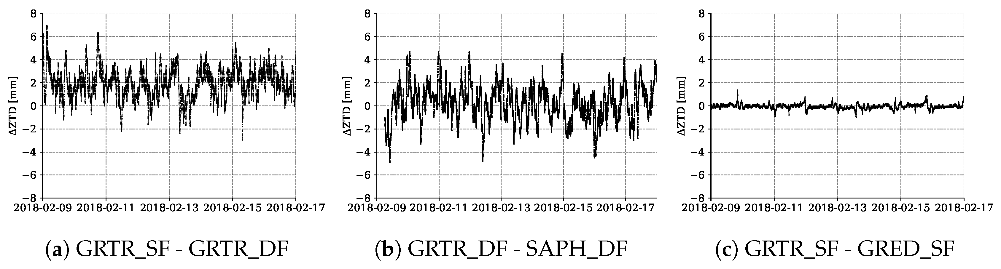
3.4. Splitting of A Geodetic Antenna to Different Receiver Types (Italy)

From GNSS basics, we know that the receiver itself and the antenna quality introduces an error to the estimations. Calibrated antennas to correct for the phase center error improve the obtained results. To further elaborate the influence of the receiver and distinguish between the SEID-introduced and the antenna error, we set up an experiment consisting of a Trimble Zephyr antenna split into a GMU (ublox LEA-M8T single-frequency receiver), a Trimble BD930 receiver (geodetic dual-frequency), and an experimental low-cost dual-frequency receiver, developed by Saphyrion Sagl, capable of tracking L1 and L2C signals. An observation period from 9 to 17 February 2018 was selected. The location of the experimental setup and the SEID-reference stations used are depicted in Figure 8.

GRTR is the dual-frequency reference station, GRED is the u-blox LEA-M8T single-frequency receiver (same as GMU from the prior experiments), and SAPH is the experimental low-cost dual-frequency receiver. All units obtain the same antenna input signal from the geodetic GRTR antenna, through a GPS Source 4-way splitter. For our analysis, we utilized the SEID reference stations LUIN, PAV2, and CATU. They are part of the NetGEO [33] network and are located within 10–50 km from the experimental setup. After synthesizing a single-frequency dataset from GRTR (GRTR_SF), we applied the SEID algorithm to the single-frequency datasets (GRTR_SF and GRED). On all datasets, the PPP was performed to obtain ZTD estimations at the locations. Contrary to the previous computations, this analysis utilized goGPS version 0.6.0, which is based on a joint least-squares adjustment. Figure 9 depicts the differences between selected time series.

Figure 9a shows the differences between the synthesized dataset GRTR_SF and its dual-frequency counterpart GRTR_DF. A bias of 1.99 mm and an RMSE of 2.40 mm is present. The comparison between the geodetic grade GRTR_DF and the experimental cost-efficient dual-frequency receiver (Figure 9b) yields an RMSE of 1.58 mm. No significant bias is visible. Figure 9c shows the differences between the SEID-generated single-frequency ZTD estimations (GRTR_SF and GRED_SF). The comparison yields an RMSE of 0.20 mm.

4. Discussion

4.1. Inter-Comparison of Reference Datasets and Analysis of the Software-Related Error

For the IGS network stations, various ZTD reference datasets from different providers are available. In our experiment, we conducted an inter-comparison between 5 analysis center outputs. The results depict a very good agreement between these yielding standard deviations between 2 and 4 mm. The variation between the reference datasets corresponds well to the uncertainty of 4 mm of the IGS troposphere products compared to other independent measurement techniques like radiosondes or numerical weather models [28]. However, the goGPS-processed results highlight differences between the goGPS PPP estimations and the available ZTD reference datasets. In our experiment, the goGPS PPP version introduced a 4 mm ZTD bias to the dual-frequency PPP solution. A part of this error may be caused by using a 10 degree elevation cut-off angle instead of 7 degrees as used in the IGS reference dataset. The comparison between the PPP-only (DLF1_DF) and the IGS dataset demonstrated an RMSE of 7 mm. This effect is mainly caused by the software-introduced bias and exceeds the 4 mm error range by the IGS troposphere products. It suggests that there is still room for improvements to the processing engine. However, the software is continuously developing, and the results are constantly improved by implementing additional model functions. In the upcoming release, the processing will switch from using a Kalman filter to a joint least-squares adjustment. This version is currently in an experimental phase. However, initial results (see Section 3.4) from the least-squares version suggest a significant improvement of the ZTD estimation accuracy. Even though the original dual-frequency ZTD estimations are subject to be improved by utilizing another PPP analysis tool, driven by the observed ZTD variation the results suggest that the goGPS estimations can be used to representatively compare the ZTD estimations among each another. Using a different processing engine will not significantly influence the investigated variations.

4.2. SEID DPGA Experiment and Antenna Impact

The conducted SEID experiment using the DPGA constellation with distances between 50 and 80 km demonstrate the successful application to our domain. The RMSE of 4 mm between the DLF1_SF and its dual-frequency counterpart validate the results from prior studies by, e.g., Deng et al. [14]. DLF1_DF and DLF1_SF use the same geodetic-grade antenna and antenna phase center corrections. Since they share the same receiver, antenna, and configuration parameters, the error between these two is entirely introduced by the SEID network interpolation and demonstrates a reasonable accuracy. The error may be introduced by loss of lock, cycle slips, or the irregular nature of the ionosphere. The ZTD results from the newly placed single-frequency stations GMU and UBX are generally noisier. The GMU, being equipped with a Tallysman antenna and u-blox LEA-M8T receiver, demonstrated a slight performance decrease compared to the synthesized dataset. The GMU contains fewer data points than the UBX device, because, especially at the end of the year, the GMU suffered technical problems caused by the insufficient power supply generated by the solar panels during winter. GMU and UBX are equipped with a similar receiver type (respectively, u-blox LEA-M8T and u-blox NEO-M8T), are co-located and use the same ionosphere correction sources. However, the UBX site is affected by a systematic bias (about 6 mm), which is presumably caused by an increased multipath effect due to the lower quality antenna. This suggests that the antenna type and placement has a major influence on the precision. The authors of Pesyna et al. [34] report that patch antennas are characterized by a less effective signal reception and suffer more from multipath effects than geodetic-grade antennas. The antenna is a simple patch antenna and shielded by a metal plate on the ground. The horizontal placement on the rooftop may be a reason for this effect. The DPGA SEID experiment demonstrated a successful application of the SEID model to single-frequency receivers with standard deviations of the ZTD error between 4 and 5 mm. A decrease in the outer network station distance using an even denser network (e.g., the Japanese GEONET or existing commercial GNSS networks) could even further improve the results. However, not all regions on the Earth, such as Europe, North America, and Japan, provide such a dense network of dual-frequency GNSS receivers. Areas that will benefit most from a densification with cost-efficient single-frequency receivers are often characterized by a much coarser reference network.

4.3. SEID EUREF Experiment

Utilizing the EUREF stations with distances between 200 and 300 km as SEID references allowed us to experimentally investigate the impact of significantly longer station distances on the ZTD estimations. The comparison between DLF1_DF and DLF1_SF indicated an ionospheric error and yielded an RMSE of 10 mm. The overall character of the data shows more variation, which results in fewer outliers. The results also suggest that the GMU reaches a similar precision as the DLF1_SF dataset. However, the GMU and UBX stations have data only available from 1 September 2017 onwards, whereas the DLF1_SF provides data throughout the year. The higher ZTD values in summer are missing for GMU and UBX. A decrease in these stations’ performance may be found if the full observation period is considered. The majority of the outliers at the experimental setup are presumably caused by hardware errors, inconsistencies during the pre-processing (e.g., undetected cycle slips during the SEID processing), re-initializations of the Kalman filter after missing epochs, and interpolation of the ionospheric component. The higher outliers are especially present at epochs with higher re-initialization rates that are caused by power-problems of the GMU. The GMU shows a slightly reduced removal of epochs (6.89%) compared to the DPGA case, which is presumably caused by less abrupt changes in ZTD estimations. This large reference network demonstrates that the limiting factor of the precision of the ZTD estimations is the ionospheric interpolation rather than the hardware quality. We expect that the GMU will provide comparable results with almost the same precision as the synthesized dataset since the noise introduced by the SEID model will dominate the estimations. This experiment shows that the SEID algorithm is able to provide ZTD estimations even over a SEID network with distances between 200 and 300 km to the single-frequency setup in a mid-latitude region. However, the ZTD RMSE of 10–12 mm compared to the dual-frequency estimation is just barely acceptable for the post-processed water vapor estimation.

4.4. PWV Estimations

An additional error is introduced by the conversion from ZTD to PWV by utilizing temperature and pressure data. Without co-located temperature and air pressure measurements, data from weather models may be used (e.g., Jiang et al. [35]). In this study we use observations from a nearby weather station. Due to the small distance of about 5 km and almost negligible height differences, a linear interpolation of the temperature is sufficient. However, the heterogeneous character of surface temperature caused, e.g., by effects such as urban heat island will result in additional PWV uncertainty. Having achieved PWV RMSE values between 0.6–1.05 mm (DPGA case) and 1.61–1.86 mm (EUREF case) compared to the dual-frequency reference, it must be highlighted that the errors from GMU and UBX are especially subject to increase since the summer period is missing in the analysis. The results show that cost-efficient single-frequency devices may provide beneficial PWV estimations over areas with up to 300 km SEID reference station distances. Such an application may be especially interesting for regions with limited investment capabilities and areas that show a high PWV variability and no or only very few available PWV in-situ data. Extending existing tropical GNSS monitoring networks like the Continuously Operating Caribbean GPS Observational Network (COCONet) or the Amazon Dense Network [36] could potentially improve the monitoring and forecasting of deep tropical convection. However, especially the geomagnetic anomaly over South America and equatorial regions are characterized by a stronger and more turbulent ionosphere than mid-latitudes. Additional research is required to evaluate the applicability of the SEID algorithm for such regions.

4.5. Antenna Splitting

The conducted antenna splitting experiment allowed us to distinguish between the SEID-introduced and hardware errors. The results suggest that, overall, the experimental goGPS version (version 0.6.0) improved the ZTD estimation, and the introduced bias was reduced. Initialization times at the day-boundaries were smoothed by buffering for 3 h before and after each daily file. Figure 9a demonstrates that the bias in this case is introduced by the SEID implementation. The differences illustrate entirely the error that is introduced by the SEID implementation. Compared to the DPGA and EUREF experiments, the reduced variation of the ZTD estimations results partly from the version change and partly from the decreased SEID station distances. However, correcting the mean bias will improve the RMSE significantly. The cost-efficient dual-frequency SAPH_DF station yields an RMSE of 1.58 mm. The most notable characteristic of the SAPH_DF station is that it is only able to track up to 8 GPS satellites simultaneously since it is limited by the amount of concurrent receiving channels. The ZTD deviation is introduced by the decreased receiver quality and by a less optimal satellite geometry due to the fact that only up to 8 satellites on two frequencies may be observed. Difficult environmental conditions, e.g., increased multipaths, may even further decrease the quality. Since the same ionosphere correction, antenna data and pattern correction is used for GRTR_SF and GRED_SF, Figure 9c illustrates the receiver clock and phase ambiguity error. It clearly demonstrates that low-cost single-frequency receivers are capable to track satellite signals with almost identical precision to geodetic-grade receivers. This suggests that the precision of the single-frequency units for ZTD estimations is foremost dependent on the correct modeling of the ionosphere and the antenna type.

5. Conclusions

Higher spatial resolution of water vapor measurements is required for the observation of smaller scale convective events [37]. Prior studies, e.g., by Oigawa et al. [10], demonstrate a positive impact using a high resolution GNSS-based PWV network on the rainfall forecast accuracy. The objective of this work was to evaluate the feasibility of a densification of existing GNSS networks with cost-efficient single-frequency GNSS receivers. In this study, we analyzed one year of GNSS data. We first compared the available ZTD reference datasets with each other at the experimental setup location. Secondly, we validated the ZTD estimations at our experimental setup using two different SEID reference networks and indicated the potential for PWV monitoring. Furthermore, we conducted an additional observation campaign to distinguish between the hardware and the SEID introduced errors.

We experimentally verified that the applied SEID model is able to successfully be used for water vapor estimations using cost-efficient single-frequency receivers. A clear precision degradation linked to the increasing outer network station distances was found. The SEID-processed synthesized dataset (DFL1_SF) demonstrated a ZTD RMSE of 3.93 and 10.32 mm for station distances of up to 80 and 300 km, respectively. The cost-efficient unit (GMU) indicates comparable results with RMSE values of 5.55 and 10.20 mm. The precision further decreased by the utilization of a simple patch antenna (station UBX) to RMSE values of 7.10 and 12.09 mm. A clear bias of −4.96 mm, presumably caused by the antenna type or an increased multipath effect, was observed for this receiver. Our analysis also highlighted a systematic ZTD bias of about 4 mm caused by the used goGPS version 0.4.3 compared to existing ZTD reference datasets. However, apart from the bias, the precision of the PPP ZTD estimations were found to be reliable.

The additional antenna splitting experiment conducted in Italy using the newest goGPS version 0.6.0 demonstrated a significant improvement to the ZTD estimation. However, the decreased SEID reference station distance also positively affected the ZTD errors. A ZTD RMSE of 2.40 mm was found for the synthesized single-frequency dataset (GRTR_SF) compared to its dual-frequency counterpart. A cost-efficient dual-frequency receiver that tracks only a limited number of satellites showed an RMSE of 1.58 mm in ZTD. Using only a few satellites, the satellite geometry deteriorates and the ZTD estimation may be negatively influenced. The experiment demonstrated that, using the SEID model, cost-efficient single-frequency receivers are able to provide ZTD estimations with almost negligible differences.

The study demonstrated that cost-efficient single-frequency receivers can serve as a promising complement to the presently available GNSS networks in mid-latitude regions. Cost-efficient single-frequency stations like the GMU used in this analysis are in operational use since the end of 2015. Historical data about the longevity for these recently designed units is not yet available. However, fulfilling certified industrial standards for protection against sand, dust, and water provide the best conditions for a long durability of the stations. In the framework of the TWIGA project [38], a network of such GMUs will be deployed in equatorial regions in Africa. The aim is to investigate the durability in more challenging environments and how the SEID model will perform in the equatorial region with more turbulent ionospheric conditions. The conducted experiments also demonstrate that the ZTD precision from single-frequency receivers is foremost dependent on the modeling of the ionosphere and the antenna type than on the internal hardware. However, the application of other ionospheric correction models is not discussed in detail in this analysis and a comparison to different ionospheric models must be considered for future studies.

Further work is required to utilize the multi-GNSS ability of the receivers for the SEID approach. Additional satellites combined with a denser network of GNSS receivers may be useful for GNSS-based 3D tomography. Especially GNSS tomography can be improved by using a multi-GNSS approach [39]. It must be highlighted that all shown results are post-processed PPP solutions, available with a temporal delay of at least two weeks. For an effective weather forecasting, the data needs to be available in near-real time (NRT). The use of multi-GNSS PPP utilizing NRT data from the IGS has been studied by Lu et al. [40]. Compared to the GPS-only mode, they were able to improve the accuracy of ZTD estimations by up to 22.2%.

Densified PWV networks may be used to improve the long-term accuracy of weather models, for climate analysis, or to improve model calibrations. They can be beneficial when studying particular weather events at particular sites or on a regional scale. In the framework of BRIGAID, the Rotterdam study area (The Netherlands) allows us to make use of additional existing dual-frequency stations within the city borders. The decreased reference station distances are expected to improve ionospheric modeling and to result in better PWV estimations. The target of our future work is to study the spatial variability of single-frequency-based PWV estimations and to analyze its impact on the monitoring and forecasting of convective events in that area. For this purpose, we installed a follow-up experimental single-frequency network consisting of four additional receivers.

References

1. Kiehl, J.T.; Trenberth, K.E. Earth’s Annual Global Mean Energy Budget. Bull. Am. Meteorol. Soc. 1997, 78, 197–208. [Google Scholar] [CrossRef]
2. Andrews, D. An Introduction to Atmospheric Physics; International Geophysics Series; Cambridge University Press: Cambridge, UK, 2000. [Google Scholar]
3. Seko, H.; Nakamura, H.; Shoji, Y.; Iwabuchi, T. The meso-y scale water vapor distribution associated with a thunderstorm calculated from a dense network of GPS receivers. JMSJ 2004, 82, 569–586. [Google Scholar] [CrossRef]
4. Cess, R.D.; Potter, G.L.; Blanchet, J.P.; Boer, G.J.; Del Genio, A.D.; Déqué, M.; Dymnikov, V.; Galin, V.; Gates, W.L.; Ghan, S.J.; et al. Intercomparison and interpretation of climate feedback processes in 19 atmospheric general circulation models. J. Geophys. Res. Atmos. 1990, 95, 16601–16615. [Google Scholar] [CrossRef] [Green Version]
5. Ning, T.; Wang, J.; Elgered, G.; Dick, G.; Wickert, J.; Bradke, M.; Sommer, M.; Querel, R.; Smale, D. The uncertainty of the atmospheric integrated water vapour estimated from GNSS observations. Atmos. Meas. Tech. 2016, 9, 79. [Google Scholar] [CrossRef]
6. Kuo, Y.H.; Zou, X.; Guo, Y.R. Variational assimilation of precipitable water using a nonhydrostatic mesoscale adjoint model. Part I: Moisture retrieval and sensitivity experiments. Mon. Weather Rev. 1996, 124, 122–147. [Google Scholar] [CrossRef]
7. Sato, K.; Realini, E.; Tsuda, T.; Oigawa, M.; Iwaki, Y.; Shoji, Y.; Seko, H. A high-resolution, precipitable water vapor monitoring system using a dense network of GNSS receivers. J. Dis. Res. 2013, 8, 37–47. [Google Scholar] [CrossRef]
8. Realini, E.; Sato, K.; Tsuda, T.; Oigawa, M.; Iwaki, Y.; Shoji, Y.; Seko, H. Local-scale Precipitable Water Vapor Retrieval from High-Elevation Slant Tropospheric Delays Using A Dense Network of GNSS Receivers. In IAG 150 Years. International Association of Geodesy Symposia; Rizos, C., Willis, P., Eds.; Springer: Cham, Switzerland, 2015; Volume 143, pp. 485–490. [Google Scholar]
9. GNSS Earth Observation Network System. Available online: http://datahouse1.gsi.go.jp/terras/terras_english.html (accessed on 12 September 2018).
10. Oigawa, M.; Tsuda, T.; Seko, H.; Shoji, Y.; Realini, E. Data assimilation experiment of precipitable water vapor observed by a hyper-dense GNSS receiver network using a nested NHM-LETKF system. Earth Planets Space 2018, 70, 74. [Google Scholar] [CrossRef] [Green Version]
11. Baldysz, Z.; Nykiel, G.; Figurski, M.; Araszkiewicz, A. Assessment of the Impact of GNSS Processing Strategies on the Long-Term Parameters of 20 Years IWV Time Series. Remote Sens. 2018, 10, 496. [Google Scholar] [CrossRef]
12. Deng, Z.; Bender, M.; Dick, G.; Ge, M.; Wickert, J.; Ramatschi, M.; Zou, X. Retrieving tropospheric delays from GPS networks densified with single frequency receivers. Geophys. Res. Lett. 2009, 36. [Google Scholar] [CrossRef] [Green Version]
13. Zumberge, J.; Heflin, M.; Jefferson, D.; Watkins, M.; Webb, F. Precise point positioning for the efficient and robust analysis of GPS data from large networks. J. Geophys. Res. B Solid Earth 1997, 102, 5005–5017. [Google Scholar] [CrossRef] [Green Version]
14. Deng, Z.; Bender, M.; Zus, F.; Ge, M.; Dick, G.; Ramatschi, M.; Wickert, J.; Lhnert, U.; Schön, S. Validation of tropospheric slant path delays derived from single and dual frequency GPS receivers. Radio Sci. 2011, 46, 1–11. [Google Scholar] [CrossRef]
15. GeoGuard Earth Monitoring Services. Available online: http://www.geoguard.eu/ (accessed on 16 May 2018).
16. Thayer, G. An improved equation for the radio refractive index of air. Radio Sci. 1974, 9, 803–807. [Google Scholar] [CrossRef]
17. Saastamoinen, J. Contributions to the theory of atmospheric refraction. Bull. Geod. 1972, 46, 279–298. [Google Scholar] [CrossRef]
18. Bevis, M.; Businger, S.; Herring, T.A.; Rocken, C.; Anthes, R.A.; Ware, R.H. GPS meteorology: Remote sensing of atmospheric water vapor using the global positioning system. J. Geophys. Res. Atmos. 1992, 97, 15787–15801. [Google Scholar] [CrossRef]
19. Baltink, H.K.; Van Der Marel, H.; van der Hoeven, A.G. Integrated atmospheric water vapor estimates from a regional GPS network. J. Geophys. Res. Atmos. 2002, 107. [Google Scholar] [CrossRef] [Green Version]
20. Bevis, M. GPS meteorology: Mapping zenith wet delays onto precipitable water. J. Appl. Meteorol. 1994, 33, 379–386. [Google Scholar] [CrossRef]
21. Pavlis, N.K.; Holmes, S.A.; Kenyon, S.C.; Factor, J.K. An earth gravitational model to degree 2160: EGM2008. EGU Gener. Assem. 2008, 10, 13–18. [Google Scholar]
22. Berberan-Santos, M.N.; Bodunov, E.N.; Pogliani, L. On the barometric formula. Am. J. Phys. 1997, 65, 404–412. [Google Scholar] [CrossRef]
23. Schaer, S. Mapping and predicting the Earth’s ionosphere using the Global Positioning System. Geod. Geophys. Arb. Schweiz 1999, 59. [Google Scholar]
24. Araujo-Pradere, E.; Fuller-Rowell, T.; Spencer, P.; Minter, C. Differential validation of the US-TEC model. Radio Sci. 2007, 42, RS3016. [Google Scholar] [CrossRef]
25. Estey, L.H.; Meertens, C.M. TEQC: The Multi-Purpose Toolkit for GPS/GLONASS Data. GPS Solut. 1999, 3, 42–49. [Google Scholar] [CrossRef]
26. Herrera, A.M.; Suhandri, H.F.; Realini, E.; Reguzzoni, M.; de Lacy, M.C. goGPS: Open-source MATLAB software. GPS Solut. 2016, 20, 595–603. [Google Scholar] [CrossRef]
27. Lyard, F.; Lefevre, F.; Letellier, T.; Francis, O. Modelling the global ocean tides: Modern insights from FES2004. Ocean. Dynam. 2006, 56, 394–415. [Google Scholar] [CrossRef]
28. Dow, J.; Neilan, R.; Rizos, C. The International GNSS Service in a changing landscape of Global Navigation Satellite Systems. J. Geod. 2009, 83, 191–198. [Google Scholar] [CrossRef] [Green Version]
29. Noll, C.E. The Crustal Dynamics Data Information System: A resource to support scientific analysis using space geodesy. Adv. Space Res. 2010, 45, 1421–1440. [Google Scholar] [CrossRef]
30. Blewitt, G. FTP Archive of NGL Troposphere Delay Products. Available online: ftp://gneiss.nbmg.unr.edu/trop (accessed on 16 May 2018).
31. EUREF Permanent GNSS Network. Available online: http://epncb.eu/_productsservices/troposphere/ (accessed on 16 May 2018).
32. de Haan, S. National/Regional Operational Procedures of GPS Water Vapour Networks and Agreed International Procedures; Rep WMO/TD-No. 1340; World Meteorological Organization: Geneva, Switzerland, 2006. [Google Scholar]
33. Topcon Positioning Italy. Available online: http://www.netgeo.it/ (accessed on 28 May 2018).
34. Pesyna, K.M.J.; Robert, W.H.J.; Humphreys, T.E. Centimeter positioning with a smartphone-quality GNSS antenna. In Proceedings of the ION GNSS+ Meeting, Tampa, FL, USA, 8–12 September 2014. [Google Scholar]
35. Jiang, P.; Ye, S.; Chen, D.; Liu, Y.; Xia, P. Retrieving precipitable water vapor data using GPS zenith delays and global reanalysis data in China. Remote Sens. 2016, 8, 389. [Google Scholar] [CrossRef]
36. Adams, D.K.; Fernandes, R.M.; Kursinski, E.R.; Maia, J.M.; Sapucci, L.F.; Machado, L.A.; Vitorello, I.; Monico, J.F.G.; Holub, K.L.; Gutman, S.I.; et al. A dense GNSS meteorological network for observing deep convection in the Amazon. Atmos. Sci. Lett. 2011, 12, 207–212. [Google Scholar] [CrossRef] [Green Version]
37. Barindelli, S.; Realini, E.; Venuti, G.; Fermi, A.; Gatti, A. Detection of water vapor time variations associated with heavy rain in northern Italy by geodetic and low-cost GNSS receivers. Earth Planets Space 2018, 70, 28. [Google Scholar] [CrossRef] [Green Version]
38. Transforming Weather Water Data into Value-Added Information services for Sustainable Growth in Africa. Available online: http://twiga-h2020.eu/ (accessed on 12 September 2018).
39. Dong, Z.; Jin, S. 3-D Water Vapor Tomography in Wuhan from GPS, BDS and GLONASS Observations. Remote Sens. 2018, 10, 62. [Google Scholar] [CrossRef]
40. Lu, C.; Chen, X.; Liu, G.; Dick, G.; Wickert, J.; Jiang, X.; Zheng, K.; Schuh, H. Real-Time Tropospheric Delays Retrieved from Multi-GNSS Observations and IGS Real-Time Product Streams. Remote Sens. 2017, 9, 1317. [Google Scholar] [CrossRef]
Figure 1. Positions of the SEID reference stations of the DPGA (red triangles) and EUREF (purple stars) constellations, the experimental setup in Delft (green square), and the AWS (orange cross). The sites DLF1, Geo Monitoring Unit (GMU), and u-blox NEO-M8T evaluation toolkit (UBX) are all co-located within a 10 m2 area.
Remotesensing 10 01493 g001
Figure 2. ZTD scatter plots of all post-processed reference datasets at DLF1 in 2017. The solid red line depicts the regression line. RMSE, bias, and std values are in millimeter. The r-value depicts the correlation.
Remotesensing 10 01493 g002
Figure 3. ZTD scatter plots of the IGS reference dataset, the dual-frequency PPP-processed DLF1 dataset (DLF1_DF), and the SEID-processed single-frequency data from UBX, GMU, and DLF1_SF utilizing the DPGA SEID reference network. The plots on the left depict the comparison of the goGPS estimations to the IGS reference dataset. The scatter plots on the right show the SEID and instrument errors. The observation period is from 1 January 2017 (DLF1_DF & DLF1_SF) and 1 September 2017 (GMU & UBX) until 31 December 2017. The solid red line depicts the regression line.
Remotesensing 10 01493 g003
Figure 4. ZTD scatter plots of the reference dataset IGS, the dual-frequency PPP-processed DLF1 dataset, and the SEID-processed single-frequency data from UBX, GMU, and DLF1_SF utilizing the EUREF SEID constellation. The plots on the left depict the comparison of the goGPS dual-frequency estimation to the IGS reference dataset. The scatter plots on the right show the SEID and instrument errors. The observation period is from 1 September 2017 until 31 December 2017. The solid red line depicts the regression line.
Remotesensing 10 01493 g004
Figure 5. ZTD differences between the goGPS-processed dual-frequency reference dataset and the SEID-processed single-frequency estimations DLF1_SF, GMU, and UBX. The figures at the top depict the DPGA SEID constellation results, whilst the ones on the bottom are from the EUREF SEID constellation, respectively. DLF1_SF (a) is the synthesized single-frequency dataset obtained from the IGS stations DLF1. GMU (b) and UBX (c) are the two cost-efficient single-frequency receivers utilizing different antenna types but sharing the same receiver type. A comparison period of 1 September–31 December 2017 was selected since all receivers provide observations during this period.
Remotesensing 10 01493 g005
Figure 6. Boxplots of the SEID-single-frequency ZTD differences to the DLF1_DF reference using the DPGA SEID constellation (blue) and the EUREF reference stations (orange).
Remotesensing 10 01493 g006
Figure 7. Cumulative error distribution plots of the single-frequency ZTD estimations DLF1_SF, GMU, and UBX compared to the DLF1_DF reference dataset. The figure at the left (a) depicts the DPGA SEID constellation results, while (b) is from the EUREF SEID case, respectively.
Remotesensing 10 01493 g007
Figure 8. Positions of the Italy-experiment SEID reference stations constellation (red triangles) and experimental setup (green square). The sites GRTR, GRED, and SAPH use the same Trimble Zephyr 2 antenna (TRM55971.00). GRTR is the dual-frequency receiver reference (Trimble BD930 receiver), GRED the cost-efficient single-frequency device (u-blox), and SAPH a low-cost experimental dual-frequency receiver.
Remotesensing 10 01493 g008
Figure 9. ZTD differences between GRTR_SF and GRTR_DF (a), GRTR_DF and SAPH_DF (b), and GRTR_SF - GRED_SF (c). The GRTR_SF and GRED_SF estimations are based on the SEID algorithm, whilst GRTR_DF and SAPH_DF use PPP-only.
Remotesensing 10 01493 g009