BULC-U: Sharpening Resolution and Improving Accuracy of Land-Use/Land-Cover Classifications in Google Earth Engine


Abstract

1. Introduction
2. Methods
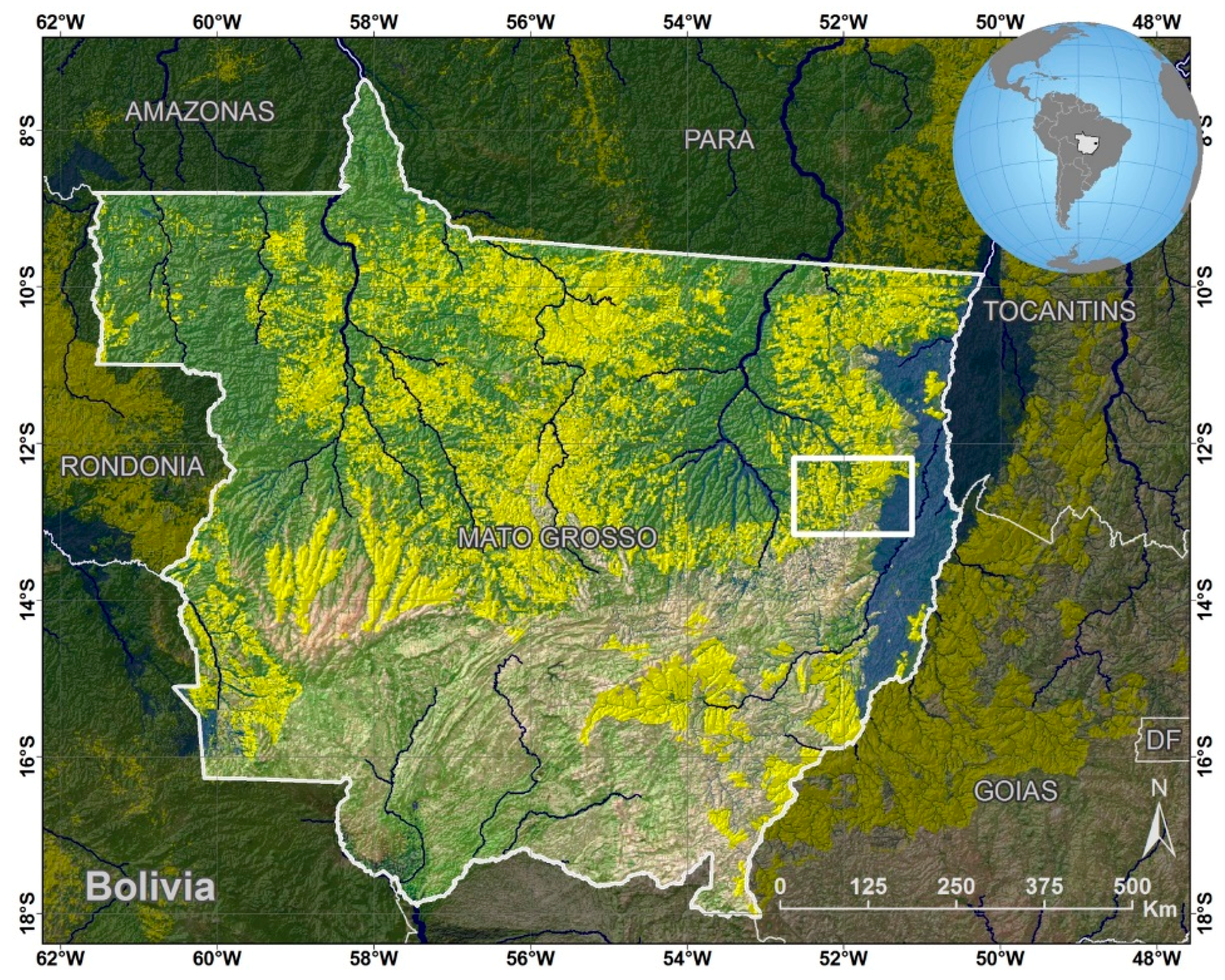
2.1. Study Area
2.2. LULC Categories
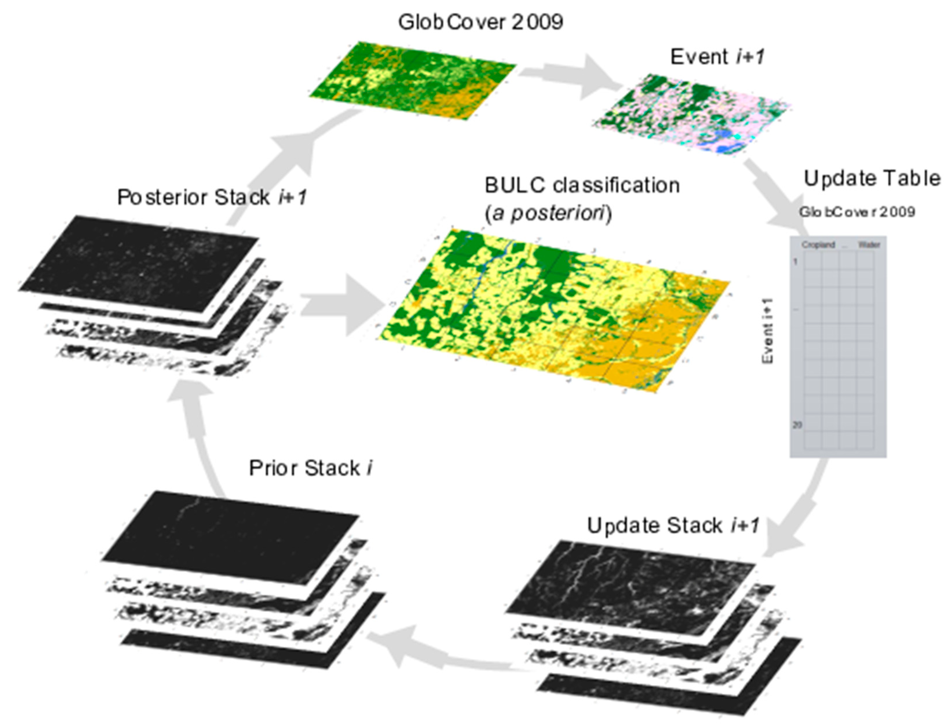
2.3. BULC-U Algorithm
2.4. GlobCover 2009
2.5. Landsat Imagery
2.6. Validation
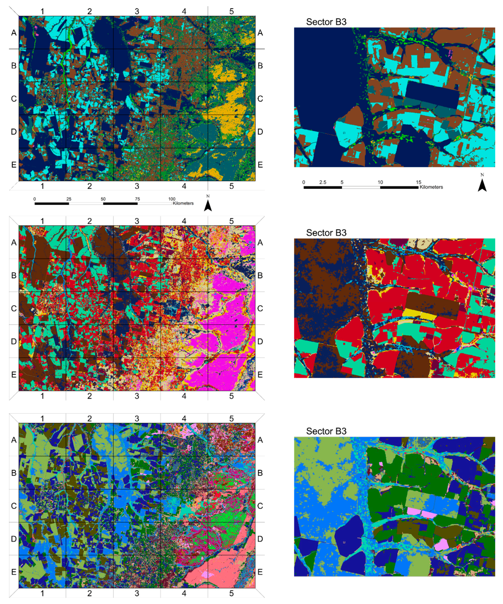
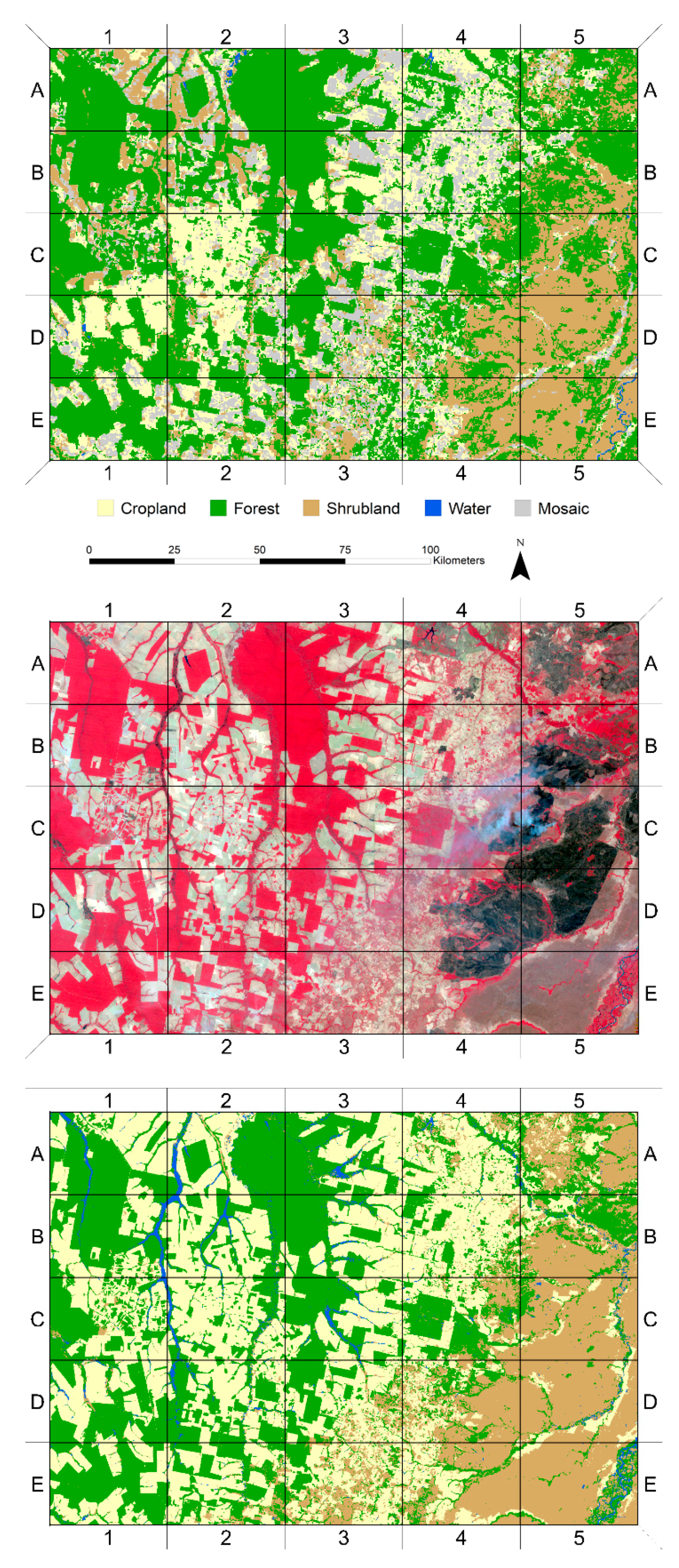
3. Results
4. Discussion
4.1. Accuracy Improvements from BULC-U
4.2. Fusing Information from Different Sensors and Projects
4.3. GlobCover 2009 as a High-Quality Data Source
4.4. Number of Unsupervised Classes for BULC-U
4.5. Strengths of the BULC-U Method
5. Conclusions
Author Contributions
Funding
Conflicts of Interest
References
- Brawn, J.D. Implications of agricultural development for tropical biodiversity. Trop. Conserv. Sci. 2017, 10. [Google Scholar] [CrossRef]
- DeFries, R.S.; Rudel, T.; Uriarte, M.; Hansen, M. Deforestation driven by urban population growth and agricultural trade in the twenty-first century. Nat. Geosci. 2010, 3, 178–181. [Google Scholar] [CrossRef]
- Costa, M.H.; Botta, A.; Cardille, J.A. Effects of large-scale changes in land cover on the discharge of the Tocantins River, Southeastern Amazonia. J. Hydrol. 2003, 283, 206–217. [Google Scholar] [CrossRef]
- Cardille, J.A.; Bennett, E.M. Tropical teleconnections. Nat. Geosci. 2010, 3, 154–155. [Google Scholar] [CrossRef]
- Turner, B.L., 2nd; Lambin, E.F.; Reenberg, A. The emergence of land change science for global environmental change and sustainability. Proc. Natl. Acad. Sci. USA 2007, 104, 20666–20671. [Google Scholar] [CrossRef] [PubMed]
- Budiharta, S.; Meijaard, E.; Erskine, P.D.; Rondinini, C.; Pacifici, M.; Wilson, K.A. Restoring degraded tropical forests for carbon and biodiversity. Environ. Res. Lett. 2014, 9, 114020. [Google Scholar] [CrossRef]
- Soares-Filho, B.; Rajao, R.; Macedo, M.; Carneiro, A.; Costa, W.; Coe, M.; Rodrigues, H.; Alencar, A. Cracking Brazil’s Forest Code. Science 2014, 344, 363–364. [Google Scholar] [CrossRef] [PubMed]
- Baccini, A.; Walker, W.; Carvalho, L.; Farina, M.; Sulla-Menashe, D.; Houghton, R.A. Tropical forests are a net carbon source based on aboveground measurements of gain and loss. Science 2017, 358, 230–233. [Google Scholar] [CrossRef] [PubMed]
- Woodcock, C.E.; Allen, R.; Anderson, M.; Belward, A.; Bindschadler, R.; Cohen, W.; Gao, F.; Goward, S.N.; Helder, D.; Helmer, E.; et al. Free access to Landsat imagery. Science 2008, 320, 1011. [Google Scholar] [CrossRef] [PubMed]
- Coppin, P.R.; Bauer, M.E. Digital change detection in forest ecosystems with remote sensing imagery. Remote Sens. Rev. 1996, 13, 207–234. [Google Scholar] [CrossRef]
- Wulder, M.A.; Coops, N.C.; Roy, D.P.; White, J.C.; Hermosilla, T. Land cover 2.0. Int. J. Remote Sens. 2018, 39, 4254–4284. [Google Scholar] [CrossRef]
- Wulder, M.A.; Masek, J.G.; Cohen, W.B.; Loveland, T.R.; Woodcock, C.E. Opening the archive: How free data has enabled the science and monitoring promise of Landsat. Remote Sens. Environ. 2012, 122, 2–10. [Google Scholar] [CrossRef]
- Zhu, Z. Change detection using Landsat time series: A review of frequencies, preprocessing, algorithms, and applications. ISPRS J. Photogramm. Remote Sens. 2017, 130, 370–384. [Google Scholar] [CrossRef]
- Verbesselt, J.; Zeileis, A.; Herold, M. Near real-time disturbance detection using satellite image time series. Remote Sens. Environ. 2012, 123, 98–108. [Google Scholar] [CrossRef]
- Giri, C.; Pengra, B.; Long, J.; Loveland, T.R. Next generation of global land cover characterization, mapping, and monitoring. Int. J. Appl. Earth Obs. Geoinf. 2013, 25, 30–37. [Google Scholar] [CrossRef]
- Yüksel, A.; Akay, A.E.; Gundogan, R. Using ASTER imagery in land use/cover classification of eastern Mediterranean landscapes according to CORINE land cover project. Sensors 2008, 8, 1237–1251. [Google Scholar] [CrossRef] [PubMed]
- Drusch, M.; Del Bello, U.; Carlier, S.; Colin, O.; Fernandez, V.; Gascon, F.; Hoersch, B.; Isola, C.; Laberinti, P.; Martimort, P. Sentinel-2: ESA’s optical high-resolution mission for GMES operational services. Remote Sens. Environ. 2012, 120, 25–36. [Google Scholar] [CrossRef]
- Li, J.; Roy, D.P. A global analysis of Sentinel-2a, Sentinel-2b and Landsat-8 data revisit intervals and implications for terrestrial monitoring. Remote Sens. 2017, 9, 902. [Google Scholar] [CrossRef]
- Loveland, T.R.; Reed, B.C.; Brown, J.F.; Ohlen, D.O.; Zhu, Z.; Yang, L.; Merchant, J.W. Development of a global land cover characteristics database and IGBP DISCover from 1 km AVHRR data. Int. J. Remote Sens. 2000, 21, 1303–1330. [Google Scholar] [CrossRef]
- Tuanmu, M.N.; Jetz, W. A global 1-km consensus land-cover product for biodiversity and ecosystem modelling. Glob. Ecol. Biogeogr. 2014, 23, 1031–1045. [Google Scholar] [CrossRef]
- Bicheron, P.; Amberg, V.; Bourg, L.; Petit, D.; Huc, M.; Miras, B.; Brockmann, C.; Hagolle, O.; Delwart, S.; Ranera, F.; et al. Geolocation Assessment of MERIS GlobCover Orthorectified Products. IEEE Trans. Geosci. Remote Sens. 2011, 49, 2972–2982. [Google Scholar] [CrossRef]
- Bicheron, P.; Henry, C.; Bontemps, S.; Partners, G. Globcover Products Description Manual; MEDIAS-France: Toulouse, France, 2008; p. 25. [Google Scholar]
- Bontemps, S.; Defourny, P.; Bogaert, E.; Arino, O.; Kalogirou, V.; Perez, J. GLOBCOVER 2009–Products Description and Validation Report; Université catholique de Louvain and European Space Agency: Louvain-la-Neuve, Belgium, 2011. [Google Scholar]
- De Sy, V.; Herold, M.; Achard, F.; Beuchle, R.; Clevers, J.; Lindquist, E.; Verchot, L. Land use patterns and related carbon losses following deforestation in South America. Environ. Res. Lett. 2015, 10, 124004. [Google Scholar] [CrossRef]
- Hu, S.; Niu, Z.; Chen, Y.; Li, L.; Zhang, H. Global wetlands: Potential distribution, wetland loss, and status. Sci. Total Environ. 2017, 586, 319–327. [Google Scholar] [CrossRef] [PubMed]
- Sloan, S.; Jenkins, C.N.; Joppa, L.N.; Gaveau, D.L.; Laurance, W.F. Remaining natural vegetation in the global biodiversity hotspots. Biol. Conserv. 2014, 177, 12–24. [Google Scholar] [CrossRef]
- Fritz, S.; See, L.; McCallum, I.; You, L.; Bun, A.; Moltchanova, E.; Duerauer, M.; Albrecht, F.; Schill, C.; Perger, C. Mapping global cropland and field size. Glob. Chang. Biol. 2015, 21, 1980–1992. [Google Scholar] [CrossRef] [PubMed]
- Liu, J.; Liu, M.; Tian, H.; Zhuang, D.; Zhang, Z.; Zhang, W.; Tang, X.; Deng, X. Spatial and temporal patterns of China’s cropland during 1990–2000: An analysis based on Landsat TM data. Remote Sens. Environ. 2005, 98, 442–456. [Google Scholar] [CrossRef]
- Seppälä, S.; Henriques, S.; Draney, M.L.; Foord, S.; Gibbons, A.T.; Gomez, L.A.; Kariko, S.; Malumbres-Olarte, J.; Milne, M.; Vink, C.J. Species conservation profiles of a random sample of world spiders I: Agelenidae to Filistatidae. Biodivers. Data J. 2018. [Google Scholar] [CrossRef] [PubMed]
- Truong, T.T.; Hardy, G.E.S.J.; Andrew, M.E. Contemporary remotely sensed data products refine invasive plants risk mapping in data poor regions. Front. Plant Sci. 2017, 8, 770. [Google Scholar] [CrossRef] [PubMed]
- Wilting, A.; Cheyne, S.M.; Mohamed, A.; Hearn, A.J.; Ross, J.; Samejima, H.; Boonratana, R.; Marshall, A.J.; Brodie, J.F.; Giordiano, A. Predicted distribution of the flat-headed cat Prionailurus planiceps (Mammalia: Carnivora: Felidae) on Borneo. Raffles Bull. Zool. 2016, 33, 173–179. [Google Scholar]
- Schulp, C.J.; Alkemade, R. Consequences of uncertainty in global-scale land cover maps for mapping ecosystem functions: An analysis of pollination efficiency. Remote Sens. 2011, 3, 2057–2075. [Google Scholar] [CrossRef]
- Schulp, C.J.; Alkemade, R.; Klein Goldewijk, K.; Petz, K. Mapping ecosystem functions and services in Eastern Europe using global-scale data sets. Int. J. Biodivers. Sci. Ecosyst. Serv. Manag. 2012, 8, 156–168. [Google Scholar] [CrossRef]
- Cardille, J.A.; Fortin, J.A. Bayesian updating of land-cover estimates in a data-rich environment. Remote Sens. Environ. 2016, 186, 234–349. [Google Scholar] [CrossRef]
- Gorelick, N.; Hancher, M.; Dixon, M.; Ilyushchenko, S.; Thau, D.; Moore, R. Google Earth Engine: Planetary-scale geospatial analysis for everyone. Remote Sens. Environ. 2017, 202, 18–27. [Google Scholar] [CrossRef]
- Blaschke, T.; Burnett, C.; Pekkarinen, A. Image segmentation methods for object-based analysis and classification. In Remote Sensing Image Analysis: Including the Spatial Domain; De Jong, S.M., Van der Meer, F.D., Eds.; Springer: Dordrecht, The Netherlands, 2004; pp. 211–236. [Google Scholar]
- Ball, G.H.; Hall, D.J. ISODATA, A Novel Method of Data Analysis and Pattern Classification; Stanford Research Institute: Menlo Park, CA, USA, 1965. [Google Scholar]
- Richards, J.A.; Jia, X. Remote Sensing Digital Image Analysis; Springer: Berlin, Germany, 2006; p. 439. [Google Scholar]
- Hansen, M.C.; Potapov, P.V.; Moore, R.; Hancher, M.; Turubanova, S.A.; Tyukavina, A.; Thau, D.; Stehman, S.V.; Goetz, S.J.; Loveland, T.R.; et al. High-resolution global maps of 21st-Century forest cover change. Science 2013, 342, 850–853. [Google Scholar] [CrossRef] [PubMed]
- Congalton, R.G. A review of assessing the accuracy of classifications of remotely sensed data. Remote Sens. Environ. 1991, 37, 35–46. [Google Scholar] [CrossRef]
- Souza, C.; Azevedo, T. MapBiomas General Handbook; MapBiomas: São Paulo, Brazil, 2017; pp. 1–23. [Google Scholar]
- Fortin, J.A.; Cardille, J.A.; Perez, E. Multi-sensor detection of forest-cover change across five decades in Mato Grosso, Brazil. Remote Sens. Environ. In Revision.


| Year | Day |
|---|---|
| 2008 | 1 June |
| 3 July | |
| 19 July | |
| 4 August | |
| 2009 | 18 June |
| 4 July | |
| 20 July | |
| 5 August | |
| 22 September | |
| 2010 | 17 May |
| 2 June | |
| 20 July | |
| 6 September |
| Land Cover Classification Accuracy | ||||
|---|---|---|---|---|
| GlobCover | BULC-U 2009 | Improvement | ||
| Overall | 69.1% | 97.5% | 28.4% | |
| Producer’s | Agriculture | 71.0% | 99.0% | 28.0% |
| Forest | 98.0% | 98.0% | 0.0% | |
| Shrubland | 67.0% | 93.0% | 26.0% | |
| Water | 40.8% | 100.0% | 59.2% | |
| User’s | Agriculture | 83.1% | 95.2% | 12.1% |
| Forest | 59.5% | 98.0% | 38.5% | |
| Shrubland | 64.4% | 97.9% | 33.5% | |
| Water | 100.0% | 99.0% | -1.0% | |
| Percentage Cover | |||
|---|---|---|---|
| GlobCover | BULC-U 2009 | Amount Loss/Gain | |
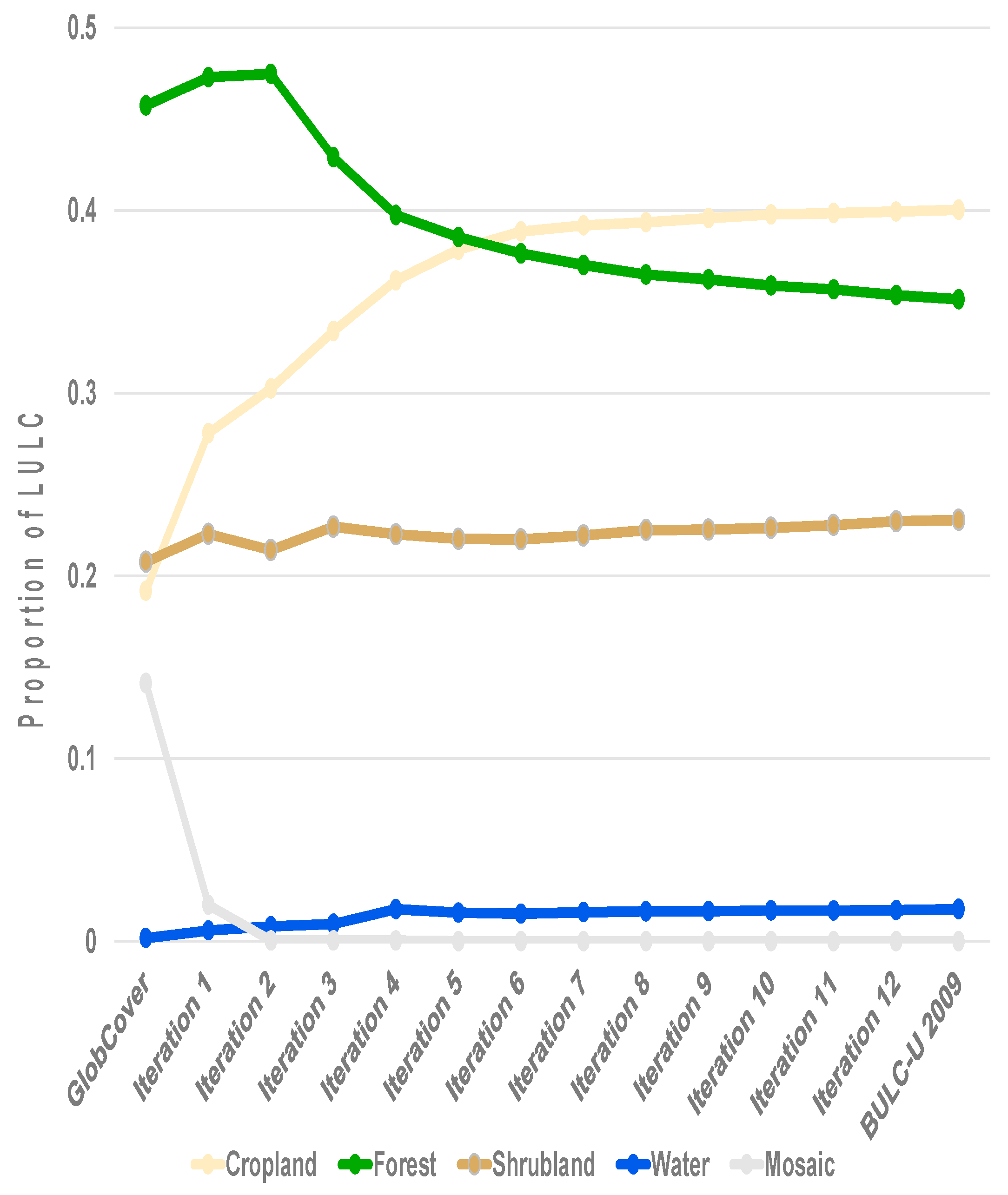
| Forest | 45.7% | 35.1% | −10.6% |
| Cropland | 19.2% | 40.0% | 20.9% |
| Shrubland | 20.8% | 23.1% | 2.3% |
| Water | 0.2% | 1.8% | 1.6% |
| Mosaic | 14.1% | 0.0% | −14.1% |
© 2018 by the authors. Licensee MDPI, Basel, Switzerland. This article is an open access article distributed under the terms and conditions of the Creative Commons Attribution (CC BY) license (http://creativecommons.org/licenses/by/4.0/).
Share and Cite
Lee, J.; Cardille, J.A.; Coe, M.T. BULC-U: Sharpening Resolution and Improving Accuracy of Land-Use/Land-Cover Classifications in Google Earth Engine. Remote Sens. 2018, 10, 1455. https://doi.org/10.3390/rs10091455
Lee J, Cardille JA, Coe MT. BULC-U: Sharpening Resolution and Improving Accuracy of Land-Use/Land-Cover Classifications in Google Earth Engine. Remote Sensing. 2018; 10(9):1455. https://doi.org/10.3390/rs10091455
Chicago/Turabian StyleLee, Jacky, Jeffrey A. Cardille, and Michael T. Coe. 2018. "BULC-U: Sharpening Resolution and Improving Accuracy of Land-Use/Land-Cover Classifications in Google Earth Engine" Remote Sensing 10, no. 9: 1455. https://doi.org/10.3390/rs10091455
APA StyleLee, J., Cardille, J. A., & Coe, M. T. (2018). BULC-U: Sharpening Resolution and Improving Accuracy of Land-Use/Land-Cover Classifications in Google Earth Engine. Remote Sensing, 10(9), 1455. https://doi.org/10.3390/rs10091455