1. Introduction
The age of technology creates the appropriate conditions for the Earth Observation (EO) domain to expand, as the multitude of on-board missions are providing almost daily measurements of land surface physical parameters [
1]. With continuous data acquisition, the generation of satellite image time series (SITS) is no longer difficult. The effort should be directed towards the development of reliable methodologies for SITS analysis [
2], since it is turning into a powerful instrument for monitoring applications.
Nevertheless, the concept of temporal behavior is sometimes difficult to perceive, as well as connecting the changes occurring over time with a specific land structure [
3]. The categories of evolution are due to latent features hidden inside the temporal signatures. The perspective offered by the multispectral images with respect to an object when analyzing a time series contributes to a better understanding of the evolution phenomena itself. Optical data provide a great amount of detail and representation with visual significance [
4]. Unfortunately, sparsity and irregular time sampling hinders a coherent analysis. Due to the sensors’ nature, multispectral data is available only on cloud-free days, such that the temporal behavior is not totally correlated with land transformations. Yet, applications such as agriculture assessment, forest monitoring, or urbanism rely on the exploration of optical SITS [
5].
Opposite to the multispectral sensors, the Synthetic Aperture Radars (SAR) are active illuminating systems, which operate in the microwave domain [
6], being one of the most exploited instruments in the remote sensing field [
7]. The large data volume of SAR systems is a consequence of the former spaceborne missions (European Remote Sensing—ERS, Envisat) whose data still can be exploited for validation of experimental concepts, with a significant number of active missions (Sentinel-1, TerraSAR-X, and TanDEM-X, COSMO-SkyMed, RADARSAT, and PALSAR). More satellites are planned to be launched in the immediate period (Sentinel-1C and 1D, COSMO-SkyMed second generation, and RADARSAT constellation), accelerating the increase of data volume. Their main advantages over optical systems rely on the fact that they can operate independently of sunlight and almost independent of weather conditions. Therefore, the generation of SAR SITS is overcoming the problems of time sampling and is not bound by cloud cover, as in the case of optical imagery. They consist of a radar mounted on a platform which moves with constant velocity relative to the illuminated scene. The sensor transmits a set of coherent impulses in the scene’s direction and integrates the reflected echoes to focus a complex bidimensional image of the scene [
8]. Compared to classical radars, SAR systems allow the 2D localization of targets in the range-azimuth plane of the focused images [
7], while the relative movement between sensor and targets leads to an azimuth resolution improvement [
9].
The lack of a direct association, valid in case of optical sensors, is compensated by some particularities of SAR imagery. The use of polarized waves allows for the assessment of a target’s structure by studying their polarimetric signatures. The employment of quadrature modulation offers the possibility to extract information related to terrain’s characteristics from the phase of the focused images by means of coherent processing. For this purpose, a wide range of coherent processing algorithms has been developed, from classical SAR interferometry to advanced multitemporal techniques. Initial approaches of SAR interferometry [
10] exploited the phase difference between two images of the same area, acquired from different sensor positions, to estimate the topography of the illuminated scene. Interferometric phase also contains a component proportional to the terrain’s displacements; this propriety represents the basics of SAR differential interferometry. In order to estimate the scene’s dislocations, a topographic component must be subtracted from the interferometric phase. This operation can be implemented either by employing an external digital elevation model (DEM)—2-pass differential interferometry, or using an elevation model estimated from a couple of SAR images—3 or 4 pass differential interferometry. Multitemporal interferometric methods study the interferometric phase variation along a dataset of multiple SAR acquisitions, allowing a better estimation of its residual component and offering the possibility to estimate and monitor the linear deformation rates of the analyzed scene over wider temporal intervals. SAR tomography [
11] combines both amplitude and phase information from a multi-baseline dataset, to reconstruct the 3D profile of the scene by estimating the reflectivity function’s variation in elevation direction.
There is an extended area in the literature for research and applications with respect to SAR SITS. Important effort has been made for the measurement of scene displacements, the most popular methods being Persistent Scatterers Interferometry (PS-InSAR) [
12,
13], small baselines subsets (SBAS) [
14], and SqueeSAR [
15]. However, there is more to develop with respect to SAR SITS processing. The analysis of scene evolution will open new perspectives for monitoring applications. In a past paper [
16], the authors used data analytics and interactive learning techniques to evaluate the manner in which a land structure was dynamically transforming over time.
One of the algorithms that proved to be very efficient for multispectral SITS analysis [
17], but also for single scene classification, regardless the type of imagery [
18,
19,
20], is the Latent Dirichlet Allocation (LDA) model. The secret lies in the way one defines analogies between the analyzed data and notions like word, document, and corpus. A generative model introduced at first to deal with text analysis, LDA can easily be adjusted to various uses, as long as relevant associations can be established. Considering the adaptability of the algorithm, this paper encourages SAR SITS handling by means of LDA modeling. This new approach aims at discovering categories of evolution to highlight the temporal behavior of land cover, as perceived by SAR systems.
The temporal behavior captured through SAR SITS is not limited to the extraction of categories of evolutions based on scene transformations. There is a perpetual character of the scene that can be emphasized using SAR SITS, where structures that are not changing over time are identified based on their coherence. The literature calls them Persistent Scatterers (PS) and they could establish a reference, nonvarying class, especially in built-up areas [
12,
13]. Often, a range-azimuth pixel from a focused SAR image can comprise the summed contributions of multiple scatterers. If a pixel presents a constant response across the SAR images dataset, it is highly probable that it contains a single, dominant target. Those points are characterized by high temporal correlation, being ideal for differential interferometry applications because they present low values of the residual component of the interferometric phase, which also offers the possibility of a more accurate atmospheric phase screen estimation. Moreover, those points are highly coherent even in image pairs with perpendicular baselines values above the critical one, which lowers the constraints on the SAR images dataset’s selection. The PS-InSAR method [
12,
13] was formulated based on those principles. This algorithm conducts an interferometric phase regression analysis in points unaffected by temporal decorrelation and is able to generate digital elevation models with submeter accuracy and estimate linear deformation rates with millimetric precision.
The stable temporal behavior of the targets analyzed within the PS-InSAR method should also be observed by the LDA classification algorithm. Consequently, all those scatterers may be included in a separate evolution class or should form multiple, separate classes. Starting from this hypothesis, the authors exploit those two envisaged components, LDA and PS-InSAR, in order to initiate an exploratory analysis of spatiotemporal SAR data with the clear purpose of discovering hidden semantics to support monitoring applications. The proposed approach was demonstrated on two SAR image time series. They were acquired using ERS and Sentinel-1 sensors over the areas of Buzau city and Constanta city, Romania, respectively.
2. Evolving Structures in SAR Imagery
When looking at a scene, the user is able to perceive well-defined structures based on visual characteristics. However, the landscape is the result of set of transformations generated by the vegetation lifecycle, geomorphological phenomena, or human activities. It is important to understand the shape of structures around us in the context of Earth surface dynamics. Temporal evolution is an important feature that must be integrated in the scene analysis together with structural features in order to define an advanced contextual meaning. While the process becomes complex, a successful data exploitation demands for scene decomposition into atoms representing primitive features. They are considered basic elements, a collection that seems rather orderless and preventing of a coherent analysis with respect to the information that can be extracted. The challenge is to discover those rules that generate meaningful feature combination, define semantics, and create knowledge and understanding for the user.
To this end, the Latent Dirichlet Allocation (LDA) model addresses the latency of scene content and uses a Bag of Words approach to discover hidden information inside the data. LDA is a generative probabilistic model able to shape semantic associations within a collection of discrete data [
21]. Although the method is designed for the peculiarities of text analysis, a collection of EO images time series, seen as a random discrete process, will respond to the algorithm’s requirements as long as relevant equivalences can be made for the parameters of the LDA model [
21]: word, document, and corpus. For this aim, the SITS will be hierarchically decomposed into basic elements representing visual words such that documents and corpus can derive without difficulty. Land surfaces similarly reflecting the echoes over the analyzed period of time will be included in the same class, with the belief that the results will picture a symbolic representation linked to the scene’s nature.
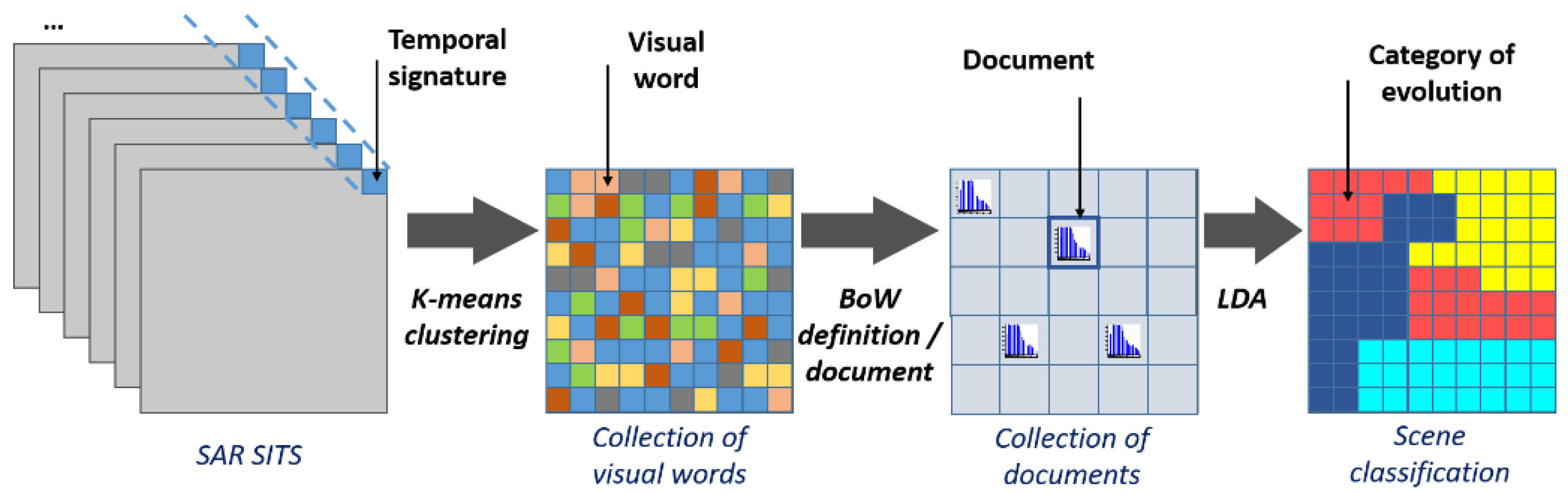
The proposed approach is presented in
Figure 1. A SITS consist of a set of EO images acquired at different moments of time over the same area, entirely covering the area, without exceeding it. From the LDA algorithm’s perspective, the first action to be completed refers to the definition of the baseline element of a SITS. We propose the temporal signature (the values of a pixel location in all the images in the time series) as the main element composing the SITS. Therefore, the SITS is decomposed in a set of R × C temporal signatures, where (R, C) is the size of the scene. By performing an unsupervised k-means [
22] clustering over the entire collection of temporal signatures, we define elements with basic understanding. As the goal is to group those pixels that share a comparable evolution over time, the similarity threshold will be forced to stay close to its maximum value. The process lies on the Euclidean distance, ensuring that the comparison between two signatures will consider measurements performed at the same moment of time (i.e., pixels (x
i,y
i) and (x
j,y
j) are first compared at moment t
1, and then at moments t
2, t
3 and so on).
The obtained k-means classes will represent visual words. In order to avoid limitations in content representations (due to a high similarity threshold), tests and previous results recommends a number of 150–250 visual words [
17]. At the next step, we associate a patch to the document. We experimentally verified that smaller patches (i.e., 5 × 5 or 10 × 10 pixels) enable better and more coherent content separation. The sequence of words defining the document is given by a Bag of Words representation of the visual words included in the patch. The corpus, a collection of documents, is associated with the analyzed SITS. Given the reduced amount of structures observable in the SAR imagery, we chose to work with 150 visual words and patches of 10 × 10 pixels.
Once the three-level hierarchy is defined, a new hidden variable, called topic, is emphasized by the LDA model. Each document will be represented as a random mixture over topics, and each topic is characterized by a distribution over words. Considering that
α and
β are the main parameters of these distributions and
θ~Dir (
α), we can compute the probability of each visual word
W to be included in the topic
z, based on the joint distribution of words and topics:
Taking into consideration all the values of
θ and
we can compute the marginal distribution of a document based on equation:
Furthermore, the probability of the corpus is measured as the product of the marginal probabilities of single documents:
where
m is the number of documents in the corpus and
the number of words in a document. LDA is a generative process where the distribution of words, documents, and corpus over the topics are incremented step by step until they converge to an acceptable error. New semantic rules were defined and unique groupings of basic elements emerged as topics relying on the temporal features. The modeling results in a scene classification, where each topic represents a category of evolution.
3. Persistent Scatterers Identification
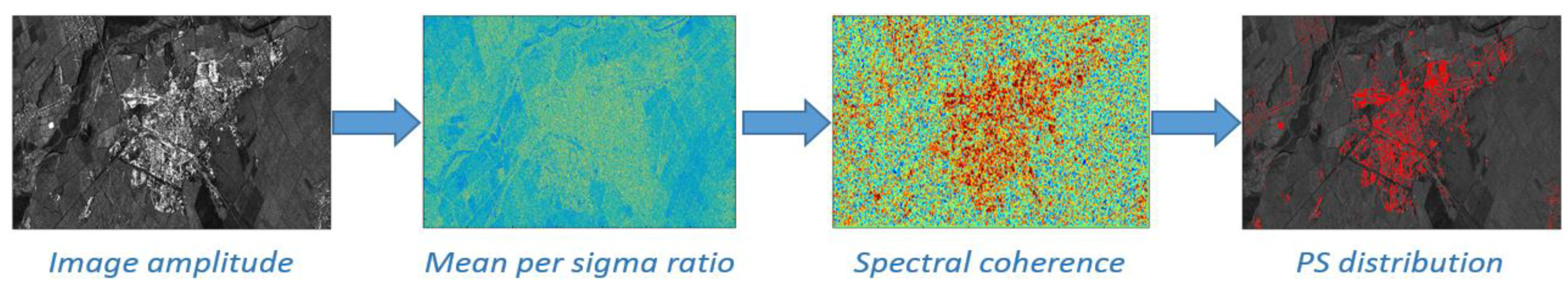
A persistent scatterers detection algorithm has been carried in this work to support a comparative study of identified PS candidates position relative to results of classification and change of detection methods. The PS identification is a two-step algorithm, consisting of the analysis of both temporal and spectral behavior of the targets [
23]. This approach is synthesized in
Figure 2.
The amplitude’s statistics are quantified by computation of the mean-per-sigma ratio in each point of the scene:
where mean
μ and standard deviation
σ are computed in discrete form, in each pixel of the scene, based on the elements of the vector
A which contains the values of resolution cell’s amplitudes along the dataset:
This mean-per-sigma ratio represents the inverse of the coefficient of variation. A stable target is considered to be present in the analyzed resolution cell if the associated MSR index of the amplitude is above unity.
The second analysis is based on the target’s spectral coherence
qx which is computed in concordance with Wiener–Hincin theorem. Elements of each dataset’s resolution cell form complex data vector
X. The number of vector’s elements is equal to number of dataset’s images. The spectral coherence
qx is therefore computed as the Fourier transform of the complex dataset’s values autocorrelation function
RXX. The Wiener–Hincin theorem is applied in discrete form:
where
N is the number of dataset’s images,
k an integer smaller than
N and variable
f denotes the frequency. In every pixel of the scene, each element
i of the data vector,
Xi can be modeled as a stochastic process. The autocorrelation function
RXX can be estimated as:
To avoid the detection of false alarms, especially in regions affected by shadowing effect, a target will be classified as PS candidate only if its amplitude value is situated above the mean of neighboring pixels. Shadowed regions are usually situated behind steep slopes and cannot be illuminated by SAR sensor. The candidate points can form the starting point of the PS-InSAR technique.
4. Experimental Setup
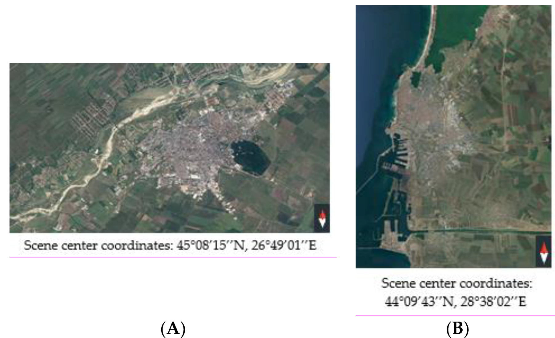
Although widely applicable, the proposed processing comes in favor of man-made structures monitoring, which usually correspond to urban areas. The dynamics of the built up area are given by the economic development of that particular region. Nevertheless, there are situations when scene displacements are influencing the land cover evolution. Landslides, earthquakes, or subsidence are the most common phenomena. In this context, we consider Buzau and Constanta cities in Romania as the test areas (
Figure 3), as they are both located near important epicenters in East Europe. The most important aspect from the point of view of the proposed experiment is that both test areas contain urban regions, which are usually characterized by a high density of PS due to the presence of built-in structures. Constanta city is located in the south-east part of Romania, in Dobrogea Plain, on the Black Sea coast. It has an area of 125 km
2, while its port extends across 30 km, being the largest harbor of Black Sea. Buzau city is located in Muntenia region, in the Baragan Plain, close to the south-east curvature of the Carpathian Mountains. Its surface equals 81 km
2. Since both cities are located in flat areas, similar classes are expected to be identified across both test regions. The surrounding areas of both cities are dominated by agricultural fields. Buzau city is crossed by the homonymous river; therefore water areas are present in both regions (in different proportions). Forest regions are also present, but not dominant, in both test areas. Considering the main objective of this work (direct comparison between detected PS and the LDA classification output), it was essential that the test scenes contain urban areas, since the stable scatterers are expected to be detected mostly in such regions. The presence of the aforementioned structures (river and sea) makes these two cities an interesting case study.
The goal is to perform a temporal analysis to identify specific categories of evolution and try to test if it is possible to provide a classification for the PS points. The process will emphasize the impact of regular low intensity earthquakes over the stability of built-up area. In order to demonstrate the efficiency of the proposed methodology, the experiments were made on data acquired with two different sensors.
4.1. Experimental Data
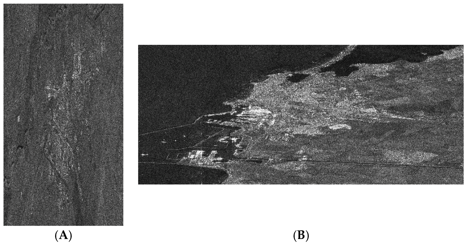
The first dataset consists of 30 images of Buzău city’s area (Romania), acquired by ERS satellites constellation between May 1995 and June 2000, in Single-Look Complex Image Mode (IMS). Even if ERS sensors are no longer active, images acquired within this mission are still used for experimental purposes, being recommended by the high range/azimuth resolution (see
Section 4.3). The dataset’s acquisition interval overlaps the period in which ERS satellites (ERS-1 and ERS-2) formed a tandem mission, although no tandem acquisitions were included in the dataset, in order to maintain an uniform characteristic for the temporal baselines. Acquisition dates of the images are synthesized in
Table 1. The dataset’s master image was selected in order to have its acquisition date (11 August 1997) located near the central point of dataset’s temporal interval, its amplitude being presented in
Figure 4A. The selected test region consists of 700 range samples and 1300 azimuth lines. The spatial resolution of the images equals 9.9 m in slant range and 5.4 m in azimuth directions.
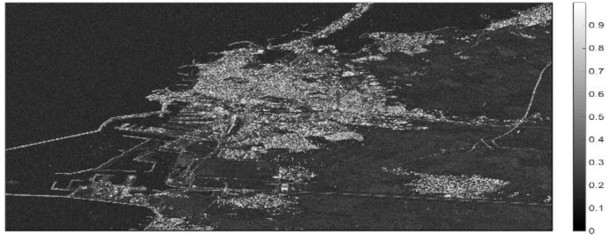
The second dataset is made of 26 images of Constanța city’s region (Romania), which are acquired in TOPS mode between October 2014 and January 2017. This interval covers the period from the availability of mission’s first acquisitions to the start of the conducted experiment. The Sentinel-1 mission is popular due to the availability of its images and the short revisit time.
Table 2 presents the acquisition dates of this dataset’s images; the reference acquisition also being chosen near the central point of the dataset’s associated temporal interval (20 November 2015). The amplitude of the master image is illustrated in
Figure 4B. The urban region chosen for analysis contains 3500 range samples and 1500 azimuth lines. This dataset presents a spatial resolution equal to 3.1 m in the slant range and 22.7 m in azimuth directions.
4.2. Preprocessing
The image preprocessing step consists mainly of the compensation of different acquisition geometries. Each image is acquired from a different position of the satellite, therefore, in each dataset, the slave acquisitions need to be resampled into the geometry of the reference image. This step is called co-registration and is usually implemented at subpixel level. Distances between the satellites’ orbits during dataset image acquisition are called perpendicular baselines.
This preprocessing step is conducted using the interferometric processing software Gamma RS [
24]. Its implementation will be performed differently for the two datasets, due to their different acquisition modes. An oversampling factor equal to 4 will be adopted in both cases, to implement the images alignment at subpixel level. Oversampling is conducted in the spectral domain.
The execution of this step is more straightforward in the case of the ERS dataset. Spatial offsets between each master–slave image pair are estimated by maximization of the amplitude’s cross-correlation
RA, which is computed in multiple sliding windows
L defined across the test region:
where
Am and
As represent the amplitude values form the master and slave images. By maximization of Equation (8) variable offsets are estimated across the scene in both range and azimuth directions. Those offsets form the basis for determination of resampling polynomials, which are used to convert the slave images to master acquisition’s geometry.
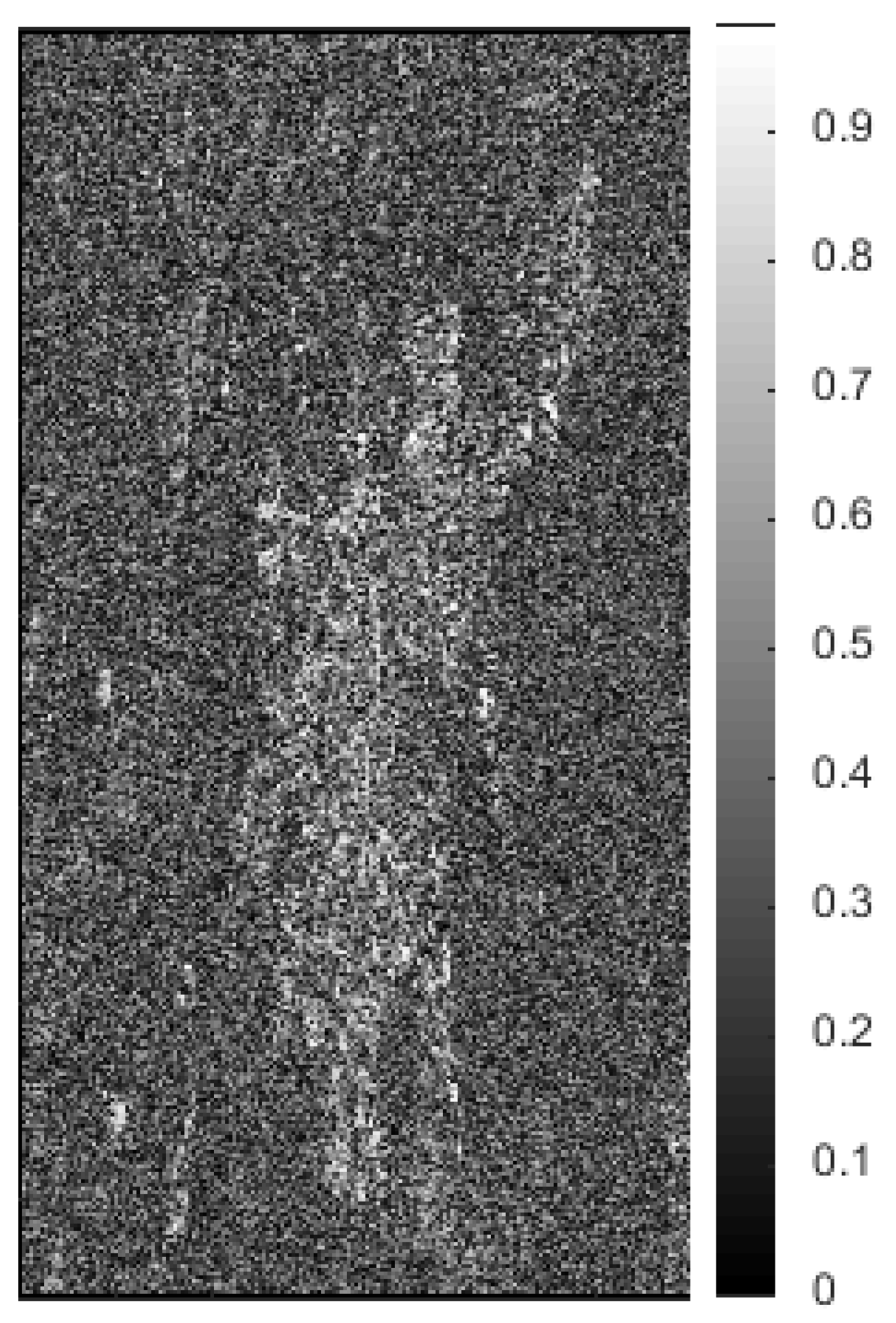
In this case, the co-registration process can be directly implemented on the test region, presented in
Figure 4-A. Validation process is conducted by computation of the amplitude’s correlation index of each co-registered master–slave image pair. Spatial variation of the mean value of this parameter, in case of ERS dataset, is shown in
Figure 5. The mean value of the amplitude’s correlation index distribution is presented here as equal to 0.33. Peak values of this parameter are present in urban regions, reaching values above 0.9. Considering that those values are close to unity, co-registration process of ERS dataset’s images is validated.
The co-registration process is more delicate in the case of the Sentinel-1 dataset. In TOPS acquisition mode, multiple swaths of the scene are simultaneously illuminated by switching the antenna between consecutive bursts. Focused images of the dataset consist of three swaths, each swath containing nine bursts. Regions covered within consecutive bursts slightly overlap at their boundaries. During illumination of each burst, the antenna beam is electronically steered in the azimuth direction. The main feature of this acquisition mode is the increased scene coverage. It is similar to the ScanSAR approach, but has the advantage of a constant SNR in the azimuth direction, across the illuminated scene.
The antenna’s steering during scene illumination induces a Doppler frequency variation across each burst, in the azimuth direction. If the image alignment is not precise, Doppler frequency shifts from bursts borders will affect further interferometric processing of the dataset, including the PS detection step based on spectral analysis.
An advantage of this dataset is that orbit related information is accurate in the case of the Sentinel-1 satellite constellation. A coarse co-registration step can be implemented by estimating a set of constant offset values in both range and azimuth directions based on orbit trajectories. This step was not conducted on the previous dataset because orbit state vectors are not reliable in case of ERS constellation.
Variable offsets will then be estimated in both range and azimuth directions, by maximization of the amplitude’s correlation index—Equation (8) this algorithm is identical to the one applied in the case of ERS images. A supplementary refinement step is considered to avoid the possible aforementioned problems: double interferograms are generated in the bursts’ overlapping regions, offsets corrections are estimated by equaling those interferograms with zero.
Therefore, it is essential, that in the case of the Sentinel-1 dataset, that the co-registration operation is implemented using at least two bursts of the images. The test region presented in the
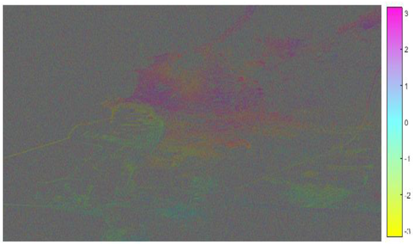
Figure 4B is situated in all the images at the division of two bursts, therefore those adjacent bursts were chosen for the alignment process. To validate the co-registration process of Sentinel-1 dataset, the interferogram of an image pair was generated. If the image alignment is precise, the burst delimitation should not be visible in the interferometric phase.
Interferometric phase generated from the images pair acquired on 20 December 2015 (reference) and 20 August 2015 (slave), from which the Earth’s curvature contribution has been subtracted, is presented in
Figure 6. The perpendicular baseline of this interferometric pair equals 160.91 m, which is a relatively high value in order to maximize the interferogram’s sensitivity to the terrain’s topography, while its temporal baseline is under three months, in order to minimize the effects of temporal decorrelation. It can be noticed that burst delimitation is not visible in the generated interferometric phase, therefore the co-registration of the dataset’s images is precise.
4.3. Comprative Analysis of Parameter’s Influence
Characteristic parameters of both datasets are synthesized in
Table 3.
Sentinel-1 dataset’s acquisition timespan is less than half that of ERS dataset’s timespan. Considering the launch date of the former mission, April 2014, is not possible yet to create a Sentinel-1 dataset which has a timespan equal to one of the ERS images. Therefore, the temporal signature of the pixels is analyzed in a larger time interval in case of ERS dataset, which should lead to more accurate results in this case. Also, both amplitude and spectral characteristics of the targets, studied for PS identification, are analyzed, in case of the two datasets, in temporal intervals with different lengths. This should not affect the PS detection process, since the stability characteristics of the persistent scatterers should be identifiable independently of the acquisition timespan of the analyzed multitemporal dataset; representing the idea behind PS-InSAR development.
The spatial dimensions of a resolution cell are lower in the case of the ERS dataset—53.46 m compared to 70.37 m for Sentinel-1 images. This decreases the probability of occurrence of the speckle phenomenon—interference between response of targets present within the same resolution cell, therefore, from this point of view, the PS detection process is slightly aided in the case of the ERS images.
The radar frequency of the two SAR datasets is similar; both sensors operated in the C band. Therefore, the additive noise has a similar influence on both datasets [
25]. Furthermore, the vegetation penetrating capabilities of both sensors are identical, so the corresponding areas should present similar behavior in case of both ERS and Sentinel-1 images.
Due to the different incidence angles of the sensors, the gap between the ground range resolutions of the two dataset’s images increases, being equal to 25.38 m for ERS and 4.92 m for Sentinel-1 set. Therefore, Sentinel-1 has a much lower value of resolution in the ground range direction, but this feature is partially annulled by its higher the azimuth resolution value.
The difference between satellite positions during image acquisition induces a shift between target spectral responses. This shift is proportional with the perpendicular baseline value. In order to be able to extract common information from a target’s response along the dataset’s multiple acquisitions, the spectrum supports of target responses across the dataset’s images must overlap, therefore the induced shift must be below a certain value. The maximum perpendicular baseline which allows common information extraction is called the critical baseline
Bcr, and is dependent on sensor to scene distance
R, radar frequency
f0 chirp bandwidth
BW, and incidence angle
θ:
The ERS dataset presents a much higher critical baseline, equal to 1041 m, compared to the Senintel-1 set, equal to 635 m. In both sets, the perpendicular baseline values are situated below the critical one, with a maximum absolute value equal to 985.2 m in case of ERS and 125 m for the Sentinel-1 set. This aspect is mostly important for LDA classification. PS detection and analysis should not be affected by the mentioned spectral shift, since the theoretical response of a stable target is represented by the Dirac impulse, hence its spectrum should have a constant value.
Dispersion of perpendicular baselines values associated with the ERS dataset is much higher compared to the Sentinel-1 images—553.54 m compared to 53.39 m. This represents a direct advantage for the latter dataset, since the aforementioned spectral shifts are lower. Higher dispersion is desirable if PS-InSAR [
13] and will be exploited on the network of detected PS, since a more precise estimation of atmospheric phase screen [
25] can be carried out.
4.4. Overview of SITS Temporal Analysis
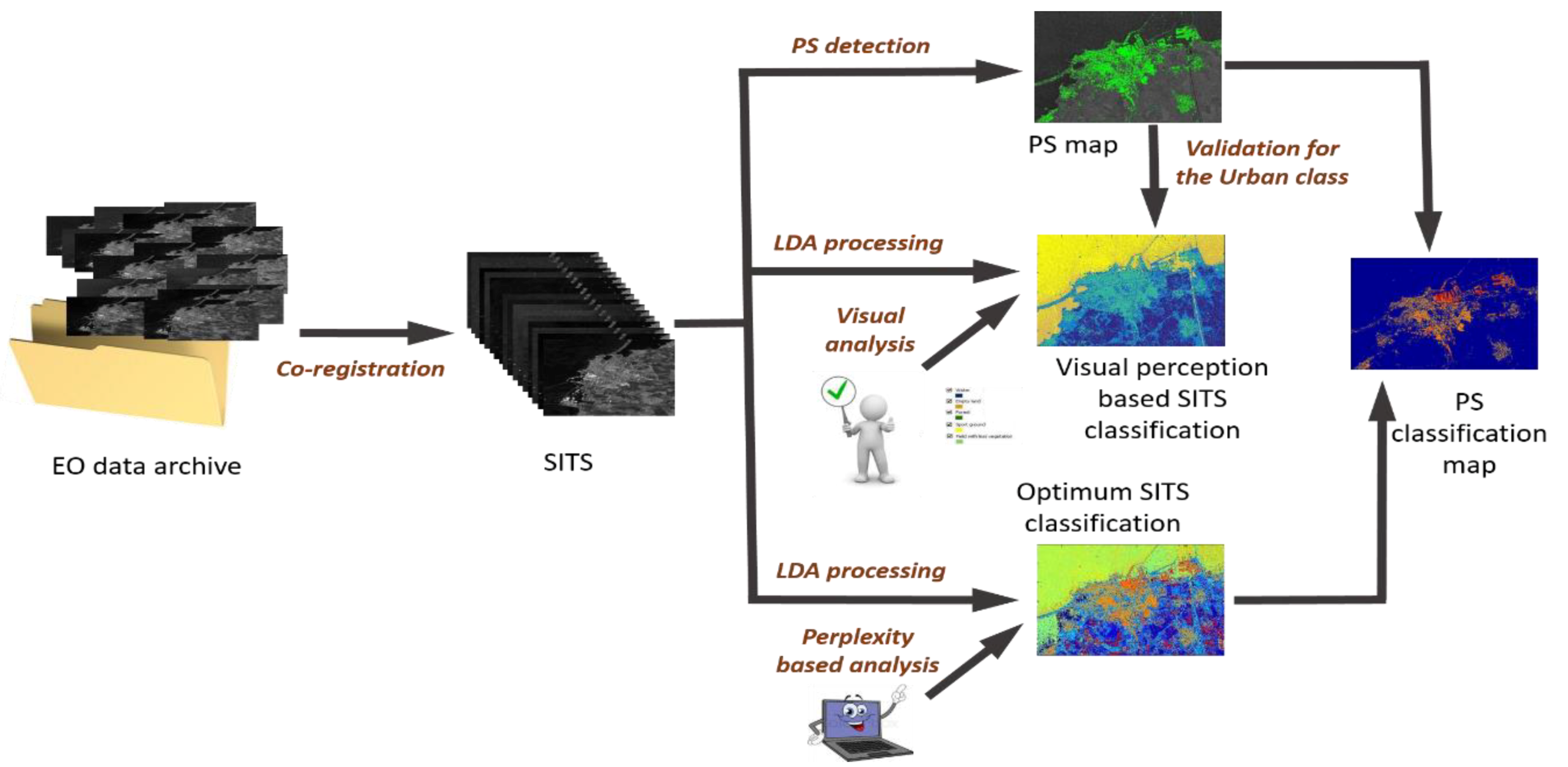
Once the preprocessing is completed, the SITS is ready for temporal analysis. The proposed methodology includes two independent processes: the PS detection (identification of persistent structures in the scene) and the categories of evolution extraction (characterization of the evolving structures in the scene), as presented in
Figure 7.
At first, we concentrate on the identification of stable targets. Amplitude statistics of each pixel values across the images dataset are computed. Points which present a MSR above 1.3 are selected in this step. For large data stacks (over 25 acquisitions, as was the case for both ERS and Sentinel-1 datasets), this method should be reliable since suitable conditions for statistics estimations are created. However, for a supplementary validation, the power spectral density of the selected points, computed according to the Wiener–Hincin theorem, is also analyzed. Points with unstable spectral phases were eliminated. From the retrained points, those which present an amplitude higher than the mean of the neighboring points will form the final PS set. Stable targets are expected to be found in areas characterized by high temporal correlation, pointing out to stable structures from the urban area. This approach could provide a reference for the scene classification and it can be used to verify the precision in urban area delimitation.
In order to differentiate the structures in the scene based on their transformation over time, we use the LDA analysis on the SITS to define categories of evolution. This kind of information is hidden to human perception, as a visual interpretation is hard to perform in this respect. All the images in the time series must be observed at the same time in order to understand if any transformation occurred in the area and to establish the extent of it with respect to the structures on the ground.
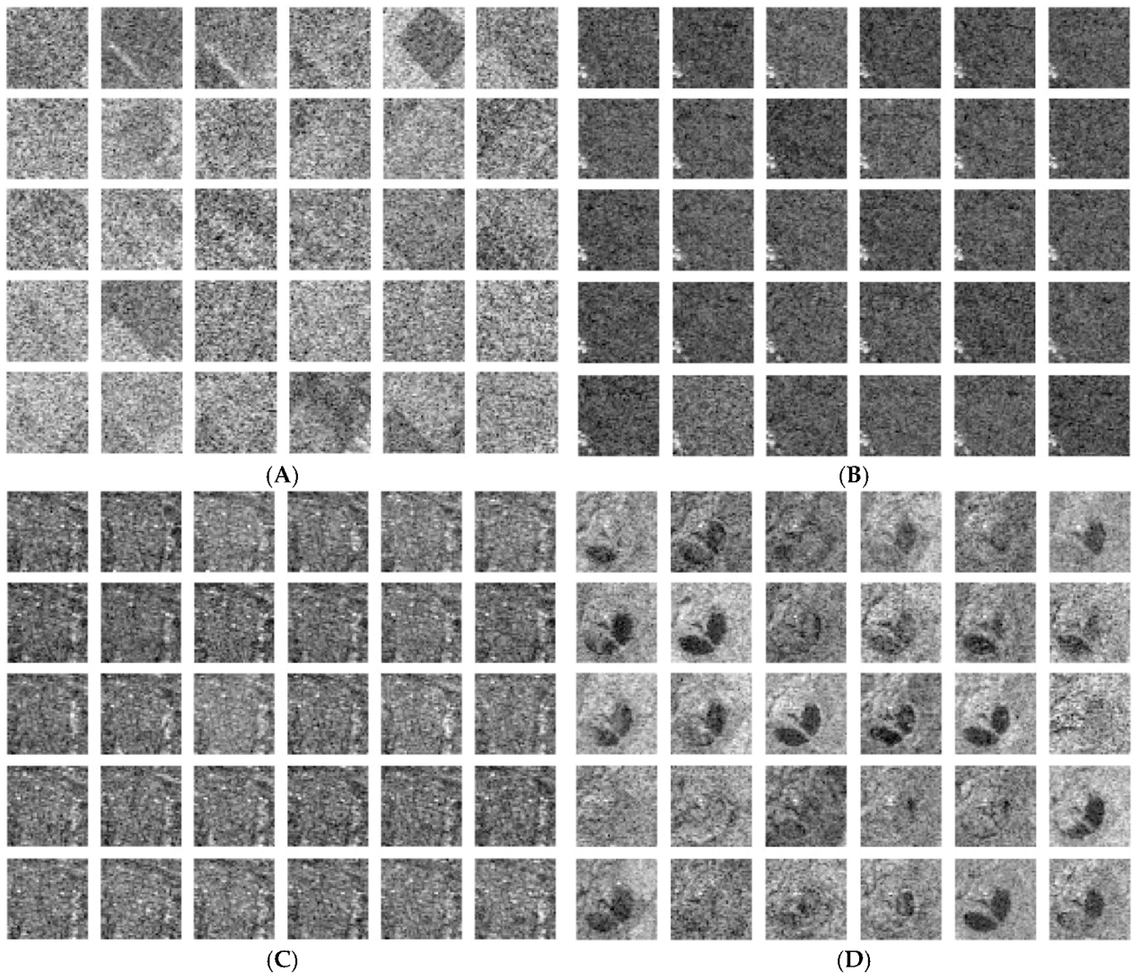
Figure 8 illustrates four categories of evolution. In these particular examples, whether the urban and forest areas present no major transformations, both agriculture and water show significant variations within a specific period of time. During SITS analysis, the focus shall turn towards of land transformations that might appear over the analyzed period.
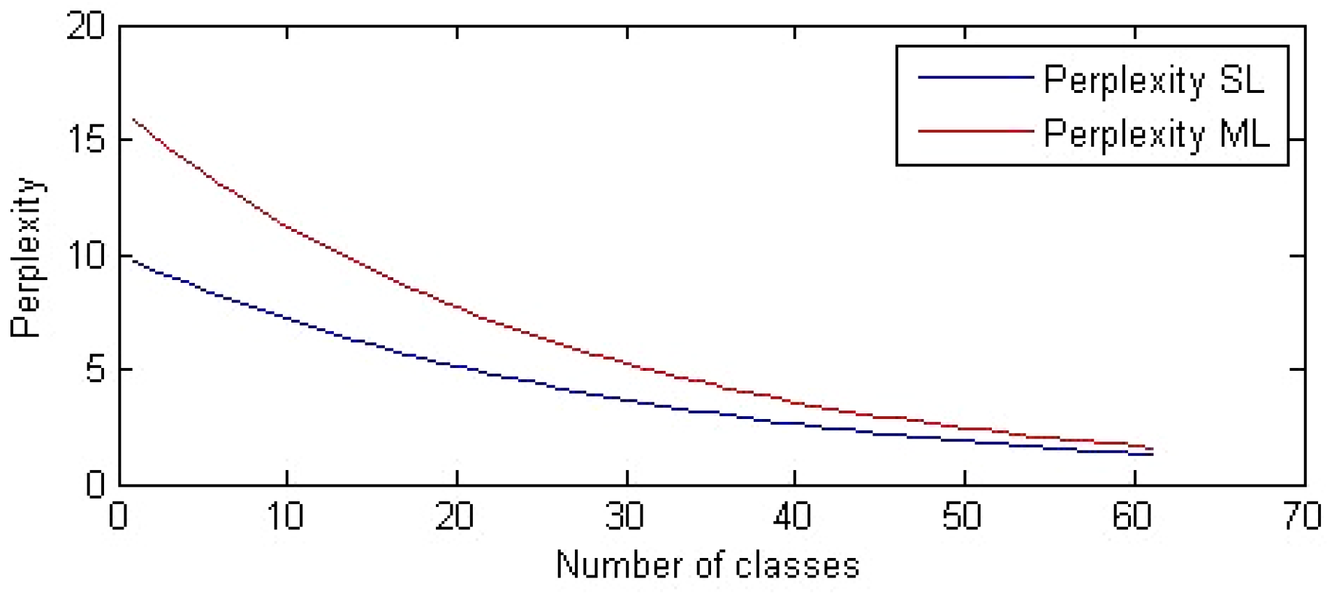
We propose two approaches for the LDA classification: at global level (where we target evolutions matching the structures on the ground distinguishable by visual perception) and at local level (where we plan to determine the set of elementary categories of evolution that can express the content scene variability in terms of changes). The only difference between the approaches refers to the selection process of the evolution categories number. In the visual approach, the number of classes is chosen based on how many categories have been perceptible to the human user in the analyzed scenes. The second approach computes the perplexity curve, which is then exploited to determine the optimal number of evolution categories. Those two methods are described below.
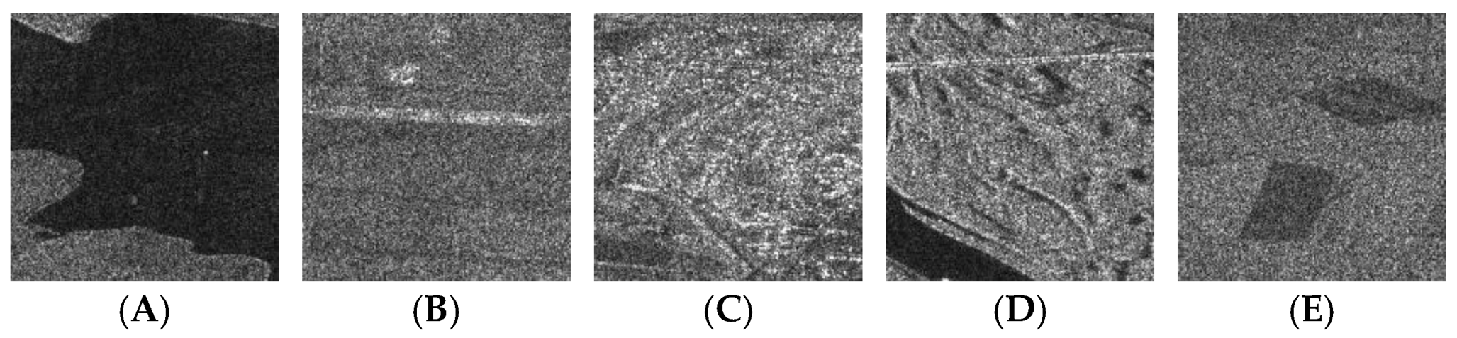
First, we plan to see how much the categories of evolution fit the semantic classes perceivable during a visual inspection of the scene: water, roads, built-up area, forest, and agricultural fields (as exemplified in
Figure 9) were identified. A strong validation measure for the case of the built-up area will be provided by the list of detected PSs.
Temporal analysis goes beyond visual land use classes; the consequences of major phenomena will be observed. Moreover, the scene rich content at a 10 m spatial resolution, combined with the SAR image complexity and the sensor’s ability to capture differently or sense multiple echoes coming from the same area at various moments of time, enable the identification of seasonal or more frequent transformations. These kinds of evolutions are multiple and hard to perceive for a human eye, but easy to separate for dedicated SITS analytics algorithms. There is no prior information regarding the correct number of potential evolutions distinguishable in a SITS. We count on the perplexity to emphasize the optimum number of categories of evolution to be extracted.
Nevertheless, a correlation between the classes observed in the scene and categories of evolution referring to the land cover modifications is not relevant. Appropriate groupings inside the scene were made based on the similarities that individual points share in terms of temporal signature. The process results in a scene classification map where the labels are assigned beyond human perception. We propose though the measure of perplexity to estimate how well the LDA model can predict the scene content based on its temporal behavior [
17]:
where
is a test set of
M documents
containing
words. The inflexion point of the perplexity curve will determine the optimum number of distinct temporal evolutions.
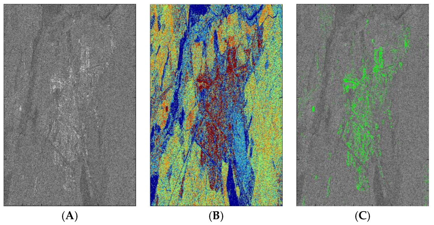
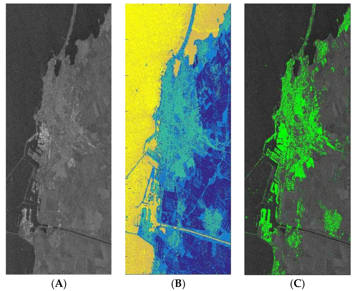
At last, the classification result is compared against the map pf detected PSs. If the number of LDA classes is low (around 5), it is likely that stable structures detected across the scene will belong to the same evolution class. Therefore, a single class will be expected to contain the vast majority of detected stable targets. If the number of classes delimited by the LDA classification is considerably higher, the set of detected stable targets will be distributed into multiple subclasses, thus allowing a supplementary classification of the PS into multiple evolution classes. Stability propriety of the detected PS is a general concept; this additional inclusion in evolution classes has the potential to be exploited in order to obtain further information related to their characteristics.
It can be noticed that, in order to study the temporal evolution of the scene, the LDA method requires solely on the amplitude of the dataset’s images. As previously mentioned, PS detection is based on the study of amplitude’s statistics and estimation of spectral coherence, therefore both amplitude and phase information being required in the latter case.
Like most coherent systems, SAR images can be affected by speckle noise, which is caused by the interference of electromagnetic waves reflected by multiple scatterers within the same resolution cell [
26]. The speckle effects can be reduced by noncoherent averaging, known as multi-looking, but this implies loss of spatial resolution. The comparative study of LDA analysis and PS detection was also implemented on multi-looked (ML) images, in case of both datasets. Spatial filtering is solely implemented based on image amplitude, so phase information is lost after application of ML. This aspect does not influence the LDA classification, but in this case PS detection, will be based exclusively on the amplitude’s statistics study, as phase information is lost after the ML process.
4.5. Amplitude’s Correlation Coefficient
Correlation coefficient is a subunit parameter, which can be exploited to understand the temporal evolution of the structures present in the SAR images. Pearson correlation coefficient
ρ can be computed between the amplitudes of each two consecutively-acquired images from the dataset:
where
i represents the position of the images in the dataset (sorted according to acquisition dates),
E denotes the statistical expectation,
A is the amplitude,
μ—its mean, and
σ—its standard deviation. This formula will be computed across the whole test scene, using 5 × 5 sliding windows. For a global characterization of the dataset, the pondered mean of the
ρi absolute values has been computed. The weights can be selected according to the temporal distribution of the images:
where
N is the number of dataset images,
ti represents the temporal interval between acquisitions
i and
i + 1, and
tt is the dataset acquisition timespan.
6. Conclusions
The paper presents a compound temporal analysis for SAR imagery, considering the persistent characteristics as well as the evolving Earth land cover behavior. The authors address the issue of irregular time sampling SITS and adapt a well-known generative model to deal with the particularities of SAR image content. Once the analogies for word, document, and corpus required by the LDA model were defined, the main advantage of the study presented here for SAR SITS is the possibility of eliminating the sparsity effect, which is characteristic to optical temporal series. Another advantage of the SAR temporal series exploited in this work is the ability to conduct the detection of points with stable temporal characteristics—persistent scatterers. The results of PS detection have been combined with the outputs of LDA classification in order to characterize the temporal behavior of the evolution classes. The evolving character extracted could be further used to determine the temporal behavior of persistent scatterers, included in built up areas.
The analytical approach of this manuscript highlights the evolutionary character of persistent structures in SAR data based on image time series analysis.
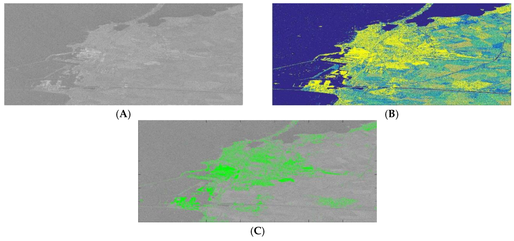
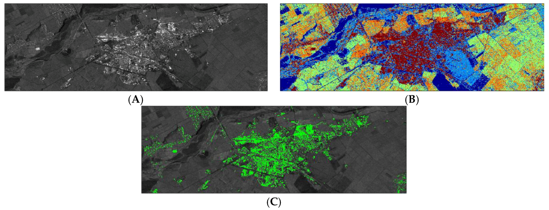
For a complete analysis, two implementations for LDA classification have been conducted, differing in the number of classes and types of transformations envisaged. In the first implementation, the number of evolution categories was determined based on the visual examination of the scene. The second implementation determined the number of classes by perplexity curve analysis, thus exceeding human perception. In the case of visual analysis, a class of stable structures, belonging mainly to built-up areas, was defined. The stable character of this class was confirmed by the PS detection results—over 90% of PS candidates are contained by this evolution class, in case of both single-look and multi-look analysis conducted on two test areas (
Table 4). Therefore, this analysis highlights the fact that, although LDA classification and PS detection methods are based on different principles, common features exist between their results.
The defining of evolution categories based on perplexity analysis leads to a significant increase of the classes number, compared to the visual based classification (from five to around 30 evolution categories in case of all analyzed scenarios). As expected, this increase leads to a supplementary classification of the detected PS into multiple evolution categories, providing a reduction in the percentages of PSs belonging to the same class, as synthesized in
Table 5. Two approaches can be defined to exploit this result. The set of PS candidates can be used to derive further information related to the temporal character of the LDA classes: evolution categories which contain high percentages of stable points can be characterized by high temporal correlation. Alternatively, this analysis can be used to derive a supplementary classification of the evolutionary character of the detected PS.
The statistical analysis of the amplitude’s mean temporal correlation coefficient leads to a supplementary validation of the conducted analysis. It confirms the stable character of the detected PS candidates (in comparison with other pixels of the test scenes). As expected, when visual-based LDA classification is conducted, the class which contains the vast majority of the stable targets presents the highest temporal correlation. Furthermore, this analysis provides supplementary information for understanding the evolutional categories: the mean temporal correlation index of each class can be exploited alongside the visual interpretation for identification of its physical structure. This process is facilitated by the diversity of the index’s mean values across the evolution classes, which vary from 0.19 in water covered areas to 0.42 in the stable points class (built-up areas).
For a better validation, the proposed analysis has been conducted on two datasets, acquired in two distinct temporal intervals by sensors with different parameters (ERS and Sentinel-1). A study of the parameters’ influence on the PS detection process is presented in this paper. The diversity of dataset temporal intervals confirms the temporal consistency of the experiment. The highest similarity between the detected PS and an LDA evolution class is present in case of single-look analysis of the ERS dataset. This is a consequence of the fact that the spatial resolution of the ERS images is better compared to Sentinel-1 acquisitions. The multi-looking process presents two main consequences: noise effect mitigation and spatial resolution loss. The second effect is predominant in the case of the ERS images (since their spatial resolution is better), leading to a PS-LDA similarity decrease. Noise suppression is dominant in the Sentinel-1 set, leading to an increase of PS-LDA similarity.
The presented experiment can also serve as a validation process for PS detection without georeferencing and visual interpretation of the results. If an LDA analysis is conducted using a limited number of classes (visual-based approach) the vast majority of the detected PS should belong to the same evolution class.
The experiments herein are some of the first attempts in the literature concerning this subject.


