Forest Variable Estimation Using a High Altitude Single Photon Lidar System

Abstract

As part of the digitalization of the forest planning process, 3D remote sensing data is an important data source. However, the demand for more detailed information with high temporal resolution and yet still being cost efficient is a challenging combination for the systems used today. A new lidar technology based on single photon counting has the possibility to meet these needs. The aim of this paper is to evaluate the new single photon lidar sensor Leica SPL100 for area-based forest variable estimations. In this study, it was found that data from the new system, operated from 3800 m above ground level, could be used for raster cell estimates with similar or slightly better accuracy than a linear system, with similar point density, operated from 400 m above ground level. The new single photon counting lidar sensor shows great potential to meet the need for efficient collection of detailed information, due to high altitude, flight speed and pulse repetition rate. Further research is needed to improve the method for extraction of information and to investigate the limitations and drawbacks with the technology. The authors emphasize solar noise filtering in forest environments and the effect of different atmospheric conditions, as interesting subjects for further research.

1. Introduction

The importance of remote sensing in forest management has significantly increased with the introduction of 3D remote sensing data. The most important 3D data source used for forest resource assessment is airborne laser scanning (ALS). ALS was developed in order to create digital elevation models (DEM). It was however soon realized that ALS was useful for estimation of forest variables as well [1,2,3]. ALS is today used in large scale to monitor forest resources and examples of nationwide coverages like Sweden is not unusual [4]. A DEM is rather stable over time and the motivation for repeated ALS acquisitions is for vegetation monitoring. A forest is a continuously changing environment and, therefore, there is regularly a need for new data. Some variables of interest, such as forest growth, are also by definition dependent on the time dimension. There is a need for a system, which can cover large areas at low cost and therefore enable high temporal resolution.

The laser scanner technology has improved over the years, for example, when it comes to pulse repetition rate, but there are still technical limitations. One factor of interest when it comes to aerial mapping with lidar is the ground sampling distance, which for a given repetition rate is a function of the flight altitude and the flight speed. For this reason, there is a clear correlation between the cost per unit area and point density. To get a reasonable cost for large area mappings like the entire Sweden [4], area-based estimation methods are used. Area-based methods do not require as high point density as single tree methods [5] to achieve sufficient estimates of forest variables. Development of a new technology called Single counting photon lidar (SPL) has the potential to meet these needs.

The most common systems used today are linear systems, where a laser pulse is emitted, reflected on a surface and the distance to the measured point is calculated from the time elapsed when the echo arrives to the sensor. The returned echo is a pulse which has a width and the shape of the received waveform depends on the target surface. Semi-porous objects like vegetation might give rise to multiple peaks of reflected energy. There are two ways of handling the received information. One way of doing it is to extract one or more distinct returns by letting energy peaks in the waveform represent distinct returns and another is to digitize the whole waveform. SPL can be described by a comparison to full waveform lidar, for which the data consist of a frequency plot of thousands of received photons at each given distance. In the case of SPL, the receiver is sensible to single photons, which means that we can measure the distance to the point of reflection for single photons. Thus, how does this comparison describe SPL? If we would be able to register a large number of photons in the same footprint as a full waveform lidar and create a frequency plot of the number of photons at each distance, we would get something similar to the full waveform [6,7]. The Leica SPL100 system (Leica Geosystems AG, Heerbrugg, Switzerland) used in this article splits the laser pulse into 100 beams, with a square regular 10 by 10 pattern. The signal from each reflected laser pulse is then imaged on to a 10 by 10 array of receivers. For each beam split, a 3D coordinate is received. In the case of a conventional lidar systems, one 3D coordinate is achieved for each pulse and the system is only capable of measuring 1D within the footprint. The sensitivity of SPL systems permits weak laser pulses, since only a few photons need to be reflected back. A good range resolution is achieved due to short pulse widths, in combination with high resolution timing detectors. A key benefit of the technique is the high repetition rate of the transmitter and short recovery time of the detectors. Short recovery time enables multiple photon measurements for each laser pulse. The properties of the SPL system result in more measured points than from a linear system under the same circumstances. More details about the sensor technology and historical development can be found elsewhere [8,9,10,11]. The Leica SPL100 system uses a laser with the wavelength of 532 nm because the single photon sensors is available for this wavelength [11]. Since 532 nm is close to the peak of solar radiation, in combination with the sensitivity of the sensor, the system is sensitive to solar noise. However, methods to filter such noise have been proposed [12,13]. Green light is also more sensitive to atmospheric scattering than the longer wavelengths used by most linear lidar systems. The effects of atmospheric conditions for the space-borne SPL sensor mounted on ICESat-2 have been simulated by Yang et al. [14]. They concluded that the atmospheric conditions have an impact on the range measurement. The suitability of the wavelength for vegetation measurements has also been discussed, but Harding et al. [15] stated that there are small differences between 532 nm systems and 1064 nm single photon systems when it comes to height of median energy and canopy cover metrics. Most of the studies with SPL data so far have looked at the possibility to generate a DEM. Stoker et al. [9] evaluated the point clouds as well as a generated DEM against field-measured ground heights. As a comparison, the same evaluation was carried out also with data from the linear lidar system Leica ALS70. They concluded that SPL performed slightly worse in terms of absolute accuracy (Root Mean Square Error, RMSE) in the point cloud assessment in non-vegetated areas (17.2 cm vs. 12.3 cm) and slightly better in vegetated areas (17.4 cm vs. 19.8 cm). For the finally constructed DEM, SPL performed better than the linear system in non-vegetated areas (14.1 cm vs. 14.6 cm) and worse in vegetated areas (40.6 cm vs. 25 cm). It should be noted that the SPL data was acquired under leaf-on conditions and data from the linear system under leaf-off conditions. Only a few studies have evaluated the SPL data for analyzes of vegetation characteristics. Harding et al. concluded that the SPL delivers data with structural measurements of high resolution and that estimations of forest variables could be made from similar metrics and with similar accuracy as conventional systems [15]. Swatantran et al. [16] compared height percentiles from SPL and linear lidar systems with field-measured tree heights. They concluded that percentile 100 from the linear system had an R${}^2$ = 0.63 and the same percentile for the SPL data showed an R${}^2$ = 0.60. They also compared percentiles between the SPL system and the linear system and concluded that percentile 100 showed an R${}^2$ = 0.83 and percentile 95 an R${}^2$ = 0.8. The results of the comparison of metrics are similar to the high correlation reported by Gwenzi et al. [17]. These studies, as well as other studies [18,19], also presents visual comparison and evaluation of canopy structure reconstruction in the 3D data, as well as the DEM characteristics. The general conclusion is that the canopies are well reconstructed in the data, mainly due to high point densities. It has been suggested that the possibility to detect understory could be higher than what could be expected from a linear systems [20]. No big differences could be noted with visual comparison of the DEM. However, it seems like production of DEM does not benefit as much from the SPL technique as the above ground measurements [19].

To our knowledge, this is one of the first studies evaluating airborne single photon lidar for forest estimations and the first one investigating the first commercial single photon-counting scanner Leica SPL100. The aim of the study is to compare area-based forest variable estimations made from the single photon counting system Leica SPL100 system, with area-based estimations made from the near infrared band from the linear system Optech Titan. Our hypothesis is that commonly used methods for area-based forest variable estimations can be used to provide estimates from SPL100 data with at least as good accuracy as from a linear distinct return system with similar point density.

2. Materials and Methods

2.1. Study Area and Sample Plots

The study area Remningstorp is located in hemi-boreal forest in southern Sweden (lat. 58${}^{\circ }$N, long. 13${}^{\circ }$E (EPSG:4326)). The test site consists of nearly 1300 ha productive forest, with active forest management. The study area contains 263 sample plots, but, due to different scanning seasons for the laser acquisitions, which meant that the broadleaf forest had leafs in one ALS acquisition but not in the other, a subset of 184 sample plots are used in this study. The criterion for inclusion in the subsample was that at least half of the stem volume should consist of evergreen coniferous trees. The study area and used sample plots are shown in Figure 1.

The subsample consisted of 42 Pine-dominated and 142 Spruce-dominated plots. The average stem volume on the plots were 213 m${}^3$/ha (SD = 160), with a Lorey’s mean height of 17.2 m (SD = 7.6) and a basal area of 22.3 m${}^2$/ha (SD = 13.6) on average. The plots have a radius of 10 m and have been located in a systematic grid pattern with the side of 200 m. The plots are located in 138 stands with a total area of 539 hectare. The plot locations were measured with a Trimble GeoXR 6000 (Trimble Inc., Sunnyvale, CA, USA), with expected sub meter accuracy. The field plot inventory started in August 2016 and ended in the spring 2017. All trees with an diameter greater than 4 cm were calipered (8816 trees) and a subsample were height measured. The forest state was calculated from the calipered trees and the sample trees using the forest planning software Heureka (Heureka 2.11.1.0, Swedish University of Agricultural Sciences, Umeå, Sweden) [21]. Local calibration of height functions has been done with functions created based on height-measured trees, from this, as well as previous inventories on the property [22]. The height functions were based on 9738 height measured trees.

2.2. ALS Data

The ALS data used in this study is a full coverage of the study area, from the new single Photon counting scanner Leica SPL100 as well as the 1064 nm wavelength from the linear system Optech Titan (Teledyne Optech, Vaughan, ON, Canada). Optech Titan also offers 532 nm and 1550 nm, but since most conventional systems used today operate at 1064 nm, this wavelength is used in this study. A transect from the SPL100 (Figure 2) and the same transect for Optech Titan (Figure 3) data are shown below. The figures illustrate the similarities in the point clouds, despite the large difference in flight altitude. Some differences in characteristics can also be seen. Metadata of the ALS acquisitions are presented in

Table 1. Metadata of the two acquisitions of ALS data.

Metadata	SPL100	Optech Titan
Flight altitude (m)	3800	400
Average point density in sample plots (point/m${}^2$)	25.4 (SD 23)	38.8 (SD 15)
Field of view (degree)	30	30
Wavelength (nm)	532	1064
Pulse repetition frequency (MHz)	6.0	0.3 (per channel)
Date of acquisition	31 October 2017	21 July 2016

.

The SPL100 data used in this study have been pre-processed by the data supplier. Processing steps done by the supplier include solar noise filtering and point cloud classification of ground and vegetation returns. Processing steps of the SPL100 data done as a part of this study were the following. Due to the scan angle, the outer boundaries of the swath do not describe the full extent of the crown in the vertical plane. The effected distance (D) from the swath boundary can be calculated with Equation (1), where H is the maximum height of the trees and $\theta$ is the scanning angle. From each flight line swath, 15 m of the outer boundaries were removed in this study, a distance which eliminates border effects to an altitude of about 56 m:

$$\mathrm{D}=\mathrm{H}·tan\theta .$$

(1)

The Optech Titan data have been classified as ground and vegetation returns and cleaned from air points as well as points under the ground. To minimize the scan angle, flight overlaps were removed by dividing the point cloud in 0.35 m grid cells in the horizontal plane. For each cell, points from the flight line with the largest scan angle were removed. Both datasets were normalized for elevation in the software LAStools (LAStools, rapidlasso GmbH, Gilching, Germany) [23]. For each sample plot, ALS returns within the sample plot were extracted and metrics were calculated with the software FUSION (FUSION, USDA Forest Service University of Washington, Seattle, WA, USA) [24]. For cover metrics as well as height percentiles, a height threshold of 1.5 m was used. The height threshold aims at eliminating influences from ground related objects such as stones. For cover metrics, this means that points over 1.5 m was expected to be canopy and only points above 1.5 m were used for calculations of height percentiles.

2.3. Outlier Removal

Sample plots with height percentile 95 lower than 1.5 m for any of the sensors, or a field-measured height lower than 1.5 m were excluded. Fifteen sample plots were removed in this step. The reason for this exclusion was to remove clear-cuts and young forest lower than the height threshold used in the calculation of metrics. In a second step, sample plots with a height difference larger than 10 m between the height percentile 95 and field-measured height were removed. This criterion resulted in five excluded sample plots, which were harvested between the field measurement and the ALS acquisition. The last step consisted of a manual exclusion of eight plots that were outliers in the data from both sensors, as well as one respectively two plots that were outliers only in the SPL100 data or the Titan data. Potential outliers for the manual exclusion were subjectively chosen through residual plots and there after visited in the field. Outliers that could be motivated with observations from the field visit were excluded. Motivations for exclusion were positioning errors, significant larger trees outside the sample plot but with part of the crown inside the sample plot and forest management between the field measurement and ALS acquisition.

2.4. Modeling

The forest variables modeled in this study were Lorey’s mean height (H), stem volume (VOL), above ground biomass (BIO), basal area (BA) and basal area weighted diameter (D). The selection of explanatory variables was made through correlation analysis, variable importance with Random Forest [25] and the variables’ contribution to coefficient of determination as well as RMSE. The selection of explanatory variables was made with stepwise inclusion, where the candidates’ correlation to the model residuals was analyzed. All FUSION metrics were tested as explanatory variables candidates. In conjunction with the analyses of R${}^2$, as well as RMSE, transformations of the response variables were made by adjusting exponents to improve linearity.

Table 2. Models used for estimation of forest variables.

Leica SPL100	Optech Titan
H = P95	H = P90
VOL${}^{0.45}$ = P95 + h95veg + e.c.m.c	VOL${}^{0.3}$ = P90 + h90veg + e.c.m.c
BIO${}^{0.2}$ = P95 + PFRA1.5 + e.c.m.c	BIO${}^{0.2}$ = P90 + PFRA1.5
BA${}^{0.3}$ = P95 + PFRA1.5 + e.c.m.c	BA${}^{0.2}$ = P90 + PFRA1.5
D = P95 + PFRA1.5	D = P90 + PFRA1.5

presents the final models. As can be seen in the table, the explanatory variables are similar, but with two differences. The models for the SPL100 sensor consist of the height percentile P95 and the Titan models the highly correlated P90. The second difference is that the e.c.m.c. metric improved the models for above ground biomass and basal area for the SPL100 sensor, but not for the Titan sensor.

Table 3. The metrics used in the models, defined and described by their corresponding names in the FUSION software.

Abbrevention	Definition	FUSION Metric
P95	The height of the point were 95 percent of the points are lower.	Elev.P95
P90	The height of the point were 90 percent of the points are lower.	Elev.P90
e.c.m.c	The qubic root of the mean qubic elevation.	Elev.CURT.mean.CUBE
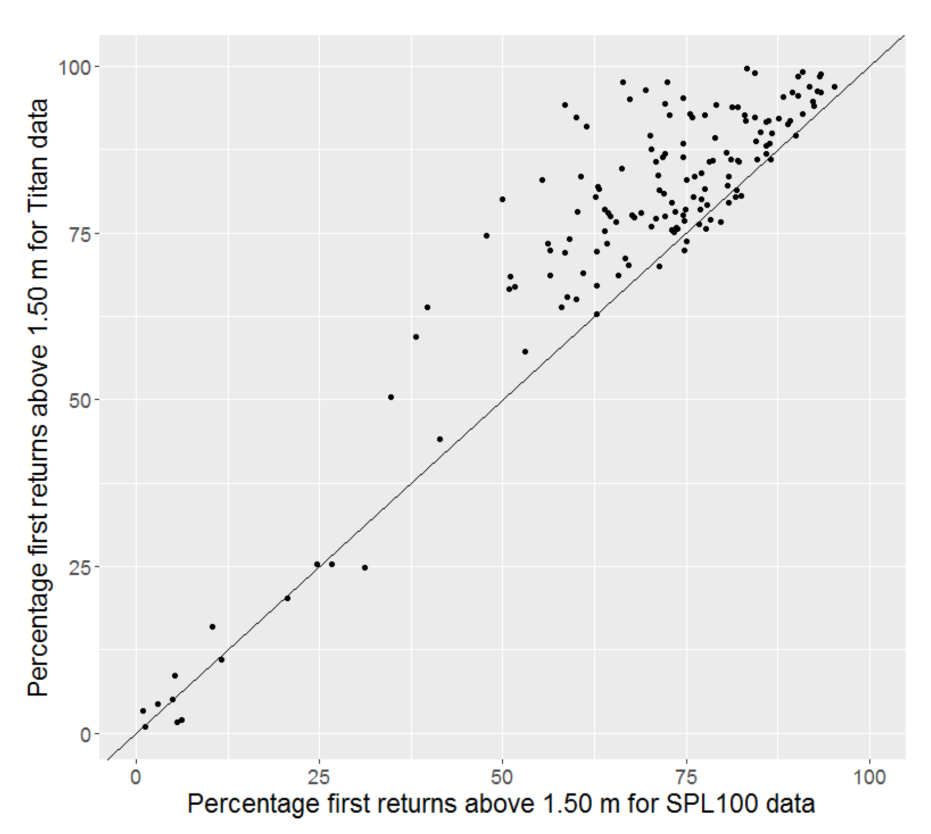
PFRA1.5	The percentage of first returned reflections 1.5 m above estimated ground.	Percentage.first.returns.above.1.50
h95veg	P95 · PFRA1.5
h90veg	P95 · PFRA1.5

presents the definition of used metrics and their corresponding names in the software. More information about the used and tested metrics can be found in the FUSION manual [24].

2.5. Accuracy Assessment

Transformed response variables have been corrected for bias [26], after back transformation, by multiplying the estimate with a correction coefficient (Q) described in Equation (2), where $Y_i$ is the field-measured value, ${\widehat{Y}}_i$ is the predicted value on sample plot i and n is the number of plots:

$$\mathrm{Q}=\frac{{\sum }_{i=1}^n{Y}_i}{{\sum }_{i=1}^n{\widehat{Y}}_i}.$$

(2)

For each variable, qualitative indicators for the estimation accuracy were calculated, using leave-one-out cross-validation on sample plot level, with Equations (3)–(6), where $\overline{Y}$ is the mean of the field measured values:

$$\mathrm{RMSE}=\sqrt[]{\frac{{\sum }_{i=1}^n{({\widehat{Y}}_i-Y_i)}^2}{n}},$$

(3)

$$\mathrm{RELATIVE}\mathrm{RMSE}=\frac{\mathrm{RMSE}}{\overline{Y}},$$

(4)

$$\mathrm{BIAS}=\frac{{\sum }_{i=1}^n({\widehat{Y}}_i-Y_i)}{n},$$

(5)

$$\mathrm{RELATIVE}\mathrm{BIAS}=\frac{\mathrm{BIAS}}{\overline{Y}}.$$

(6)

3. Results

The field-measured and estimated stem volume for the two sensors are shown in Figure 4. The left plot illustrate the relation between estimated and field measured stem volume for the SPL100 sensor and the right for the Titan sensor.

The SPL100 data resulted in slightly better estimates than for the Titan data for all variables except for basal area. None of the variables or sensors showed bias larger than 3.14 · 10${}^{-14}$. The estimation accuracy is shown in

Table 4. The table presents estimation accuracy and coefficient of determination for the two lidar systems.

Sensor	Variable	Adj.R${}^2$	RMSE	Relative RMSE (%)
	Lorey’s mean height (m)	0.96	1.14	6.11
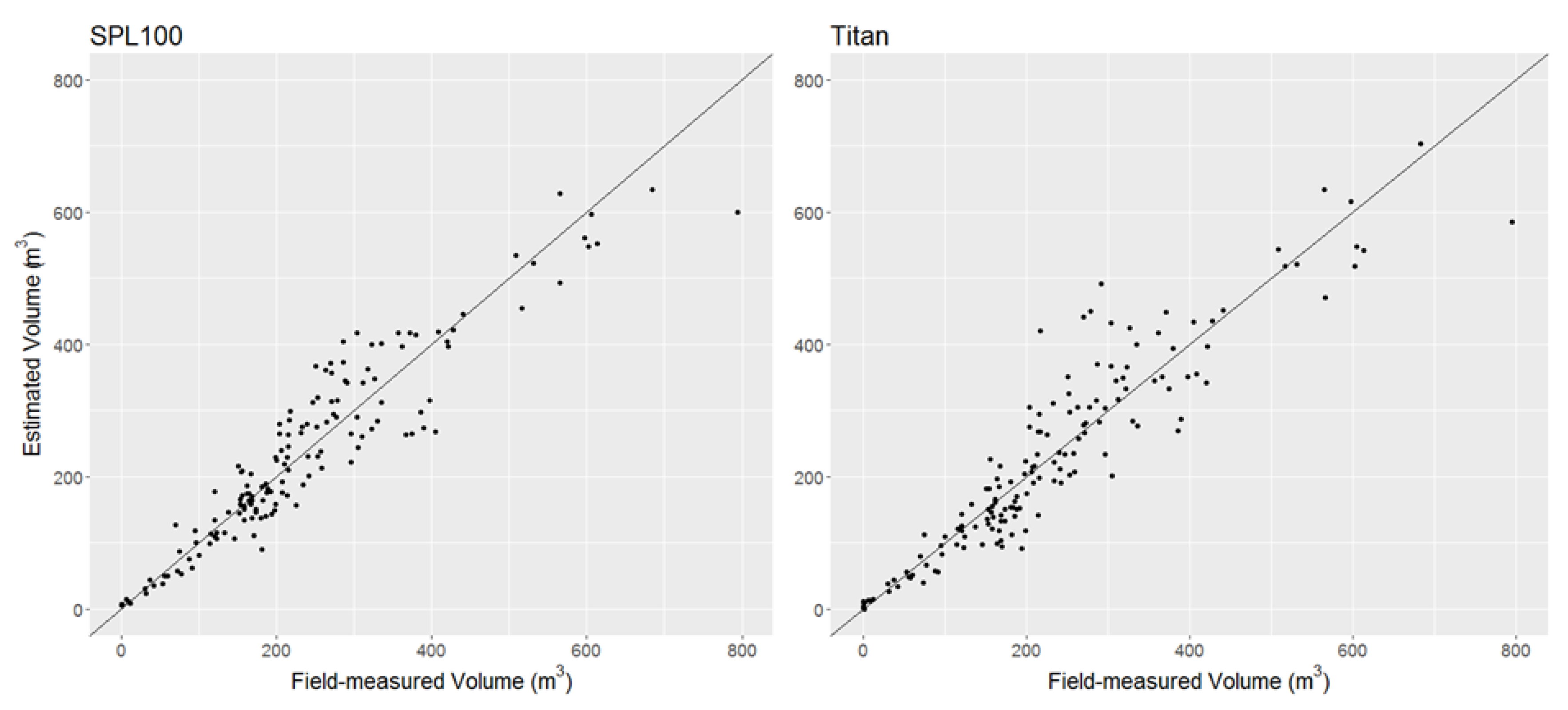
	Stem volume (m${}^3$/ha)	0.93	48.84	21.23
Leica SPL100	Above ground biomass (ton/ha)	0.93	26.90	21.27
	Basal area (m${}^2$/ha)	0.90	5.30	21.98
	Basal area weighted diameter (cm)	0.86	3.38	13.77
	Lorey’s mean height (m)	0.96	1.16	6.24
	Stem volume (m${}^3$/ha)	0.91	55.95	24.31
Optech Titan	Above ground biomass (ton/ha)	0.94	29.02	22.94
	Basal area (m${}^2$/ha)	0.93	4.80	19.90
	Basal area weighted diameter (cm)	0.85	3.46	14.10

.

An observed difference between the two datasets is the vegetation coverage metric, the percentage first return above 1.5 m. The metric seems to be saturated earlier for the Titan sensor than for the SPL100. When the Titan system almost reaches the saturation point of 100 percent vegetation points for some of the sample plots, SPL100 still has up to 40 percent of its measuring points on the ground and therefor a possibility to quantify even denser forest, which can be seen in Figure 5.

4. Discussion

An interesting fact in this study is that SPL does not seem to be saturated as fast as the Titan system when it comes to canopy cover. Densified data in the lower part of the canopy could improve the possibility to detect understory trees and therefore improve estimations in multi-layer forest, especially when single tree approaches are used. The ability to penetrate dense canopies has important benefits not only for forest variable estimations, but also for DEM generation. A similar experience of more ground points is described by Li et al. [19].

This study has focused on area-based estimations. However, area-based methods are probably not the best way for utilizing all the forest information in the SPL data. With such high point densities, single tree approaches are possible. Single tree methods have not been used in operational cases as much as area-based methods, partly due to their demands for higher point densities. The efficiency of the SPL100 could make high density data affordable even at large areas. Although we have the possibility to go down to tree level, we found it important to first validate the technology with the method most often used today. If area-based methods are the purpose for a data acquisition, lower point densities could be accepted. If this is the case, a larger field of view could be investigated, in order to further increase the productivity. Since SPL100 has a circular scan pattern, the field of view is constant and there is no mix between angles.

The use of 532 nm as operating wavelength gives rise to two issues worth mentioning. The sensitivity of the sensor in combination with the presence of the wavelength in solar radiation causes false returns to the sensor (solar noise) and the other thing is that the wavelength is sensible to atmospheric conditions. A crucial point in the processing of SPL data is therefore the separation of true measurements from solar noise. Filtering of random noise could be difficult in the canopies and there is a risk that we only filter easy noise that is not close to a canopy, or that the filtering algorithm is more efficient in certain circumstances. There is a possibility that the amount of information in the point cloud is reduced as an effect of the filtering, or, in other words, the filtering could act as a normalization of desired characteristics. This could have negative effects for area-based estimations, as well as for delineation of objects from the ALS data—for example, single tree identification. The suitability for SPL data and the filtering algorithms in single tree estimations need to be evaluated in future research. The filtering of the raw data used in this study has been carried out by the data supplier and was therefore out of our control. The results should therefore be seen as the accuracy that could be expected from preprocessed data from a commercial supplier at the moment. Algorithms for raw data processing in forested land need to be investigated in future research. The influence of atmospheric conditions and the use of green light (532 nm) have been discussed in earlier research [14], with the conclusion that the presence of cloud will affect the range measurement as well as the number of received photons. How this will effect forest variables estimations is unclear and is something that needs to be further investigated and considered in large scale applications.

The timing of the inventory and the ALS acquisitions is not ideal in this study, mainly for two reasons. The first reason is the time gap of one growing season between the inventory and the acquisition of the SPL100. If changes of the forest state would have occurred in the time gap, they could negatively affect the possibility to accurately estimate the forest state due to weaker correlation between the ALS derived metrics and the variables of interest. However, this would be a disadvantage for the SPL100 system in the comparison and hence not lead to overoptimistic results for that sensor. The second reason is that the Titan system is flown during leaf-on season while the SPL100 system is flown during leaf-off season. To minimize the risk of influences from the season, we have only used plots dominated by evergreen trees.

One of the most impressive advantages with the new SPL technology is the productivity. The systems’ capability of high flight altitudes and speed, in combination with the large number of measurement points, makes the SPL100 a revolution in the field of lidar technology. The SPL data used in this study is part of a 4800 km${}^2$ coverage, which were acquired approximately six times faster than could be expected from a conventional system, according to the data supplier. Based on the swath widths and specified flight speeds, without taking flight overlaps and flight pattern into account, SPL100 covers about 590 km${}^2$/h and the Titan system about 50 km${}^2$/h.

5. Conclusions

This study has shown that forest variables can be estimated with estimation accuracies similar or slightly higher using a single photon lidar system operated from high altitude (3800 m), compared to estimates from a conventional system, with the same point density but operated from low altitude (400 m). An advantage of the SPL100 system appears to be a better ability to penetrate dense canopies. The possibility to use SPL for forest variable estimation will increase the possibility to meet the need of detailed information with high temporal resolution for forest resource monitoring. The high flight altitude, speed and point density enable efficient areal coverage. Further research is needed to evaluate the limitations of the technology and how to extract desired information. One such technology-related issue is the sensitivity to different atmospheric conditions and the use of the wavelength 532 nm for large area applications. Regarding the extraction of information, filtering of solar noise could be a crucial point in this process. Future research should investigate methods for minimizing the negative influence of solar noise and noise filtering in forest environments.

References

- Nilsson, M. Estimation of tree heights and stand volume using an airborne lidar system. Remote Sens. Environ. 1996, 56, 1–7. [Google Scholar] [CrossRef]
- Næsset, E. Determination of mean tree height of forest stands using airborne laser scanner data. ISPRS J. Photogramm. Remote Sens. 1997, 52, 49–56. [Google Scholar] [CrossRef]
- Hyyppä, J. Detecting and estimating attributes for single trees using laser scanner. Photogramm. J. Finl. 1999, 16, 27–42. [Google Scholar]
- Nilsson, M.; Nordkvist, K.; Jonzén, J.; Lindgren, N.; Axensten, P.; Wallerman, J.; Egberth, M.; Larsson, S.; Nilsson, L.; Eriksson, J.; et al. A nationwide forest attribute map of Sweden predicted using airborne laser scanning data and field data from the National Forest Inventory. Remote Sens. Environ. 2017, 194, 447–454. [Google Scholar] [CrossRef]
- Næsset, E.; Gobakken, T.; Holmgren, J.; Hyyppä, H.; Hyyppä, J.; Maltamo, M.; Nilsson, M.; Olsson, H.; Persson, A.; Söderman, U. Laser scanning of forest resources: The nordic experience. Scand. J. For. Res. 2004, 19, 482–499. [Google Scholar] [CrossRef]
- Harding, D. Pulsed laser altimeter ranging techniques and implications for terrain mapping. In Topographic Laser Ranging and Scanning; CRC Press: Boca Raton, FL, USA, 2018; pp. 201–220. [Google Scholar]
- Jutzi, B. Less Photons for More LiDAR? A Review from Multi-Photon Detection to Single Photon Detection. In Proceedings of the 56th Photogrammetric Week (PhoWo), University of Stuttgart, Stuttgart, Germany, 11–15 September 2017. [Google Scholar]
- Degnan, J.J. Photon-counting multikilohertz microlaser altimeters for airborne and spaceborne topographic measurements. J. Geodyn. 2002, 34, 503–549. [Google Scholar] [CrossRef]
- Stoker, J.; Abdullah, Q.; Nayegandhi, A.; Winehouse, J. Evaluation of Single Photon and Geiger Mode Lidar for the 3D Elevation Program. Remote Sens. 2016, 8, 767. [Google Scholar] [CrossRef]
- Degnan, J.; McGarry, J.; Zagwodzki, T.; Dabney, P.; Geiger, J.; Chabot, R.; Steggerda, C.; Marzouk, J.; Chu, A. Design and performance of an airborne multikilohertz photon-counting microlaser altimeter. Int. Arch. Photogramm. Remote Sens. Spat. Inf. Sci. 2001, 34, 9–16. [Google Scholar]
- Degnan, J. Scanning, Multibeam, Single Photon Lidars for Rapid, Large Scale, High Resolution, Topographic and Bathymetric Mapping. Remote Sens. 2016, 8, 958. [Google Scholar] [CrossRef]
- Tang, H.; Swatantran, A.; Barrett, T.; DeCola, P.; Dubayah, R. Voxel-Based Spatial Filtering Method for Canopy Height Retrieval from Airborne Single-Photon Lidar. Remote Sens. 2016, 8, 771. [Google Scholar] [CrossRef]
- Wang, X.; Glennie, C.; Pan, Z. An Adaptive Ellipsoid Searching Filter for Airborne Single-Photon Lidar. IEEE Geosci. Remote Sens. Lett. 2017, 14, 1258–1262. [Google Scholar] [CrossRef]
- Yang, Y.; Marshak, A.; Palm, S.P.; Várnai, T.; Wiscombe, W.J. Cloud impact on surface altimetry from a spaceborne 532-nm micropulse photon-counting lidar: System modeling for cloudy and clear atmospheres. IEEE Trans. Geosci. Remote Sens. 2011, 49, 4910–4919. [Google Scholar] [CrossRef]
- Harding, D.J.; Dabney, P.W.; Valett, S. Polarimetric, two-color, photon-counting laser altimeter measurements of forest canopy structure. In Proceedings of the SPIE 8286, International Symposium on Lidar and Radar Mapping 2011: Technologies and Applications, Nanjing, China, 24 October 2011. [Google Scholar]
- Swatantran, A.; Tang, H.; Barrett, T.; DeCola, P.; Dubayah, R. Rapid, High-Resolution Forest Structure and Terrain Mapping over Large Areas using Single Photon Lidar. Sci. Rep. 2016, 6, 28277. [Google Scholar] [CrossRef] [PubMed]
- Gwenzi, D.; Lefsky, M.A. Prospects of photon counting lidar for savanna ecosystem structural studies. ISPRS Int. Arch. Photogramm. Remote Sens. Spat. Inf. Sci. 2014, XL-1, 141–147. [Google Scholar] [CrossRef]
- Turner, M.D.; Kamerman, G.W.; Wasiczko Thomas, L.M.; Spillar, E.J.; Kim, A.M.; Runyon, S.C.; Olsen, R.C. Comparison of full-waveform, single-photon sensitive, and discrete analog LIDAR data. In Proceedings of the SPIE 9465, Laser Radar Technology and Applications XX, and Atmospheric Propagation XII, 946501, Baltimore, MD, USA, 20–24 April 2015. [Google Scholar]
- Li, Q.; Degnan, J.; Barrett, T.; Shan, J. First evaluation on single photon-sensitive lidar data. Photogramm. Eng. Remote Sens. 2016, 82, 455–463. [Google Scholar] [CrossRef]
- Rosette, J.; Field, C.; Nelson, R.; DeCola, P.; Cook, B. A new photon-counting lidar system for vegetation analysis. In Proceedings of the 11th International Conference on LiDAR Applications for Assessing Forest Ecosystems (SilviLaser 2011), Hobart, Australia, 16–20 October 2011. [Google Scholar]
- Wikström, P.; Edenius, L.; Elfving, B.; Eriksson, L.O.; Lämås, T.; Sonesson, J.; Öhman, K.; Wallerman, J.; Waller, C.; Klintebäck, F. The Heureka forestry decision support system: An overview. Math. Comput. For. Nat. Resour. Sci. 2011, 3, 87–94. [Google Scholar]
- Wallerman, J.; Nyström, K.; Andersson, T.; Holmgren, J.; Lindgren, N.; Fransson, J. Surveys at Remningstorp in Years 2003–2014 (Department Report); Technical Report; SLU, Department of Forest Resource Management: Umeå, Sweden, 2017; in preparation. [Google Scholar]
- Isenburg, M. LAStools–Efficient Tools for LiDAR Processing. Available online: https://rapidlasso.com/lastools/ (accessed on 10 December 2017).
- McGaughey, R.J. FUSION/LDV: Software for LIDAR Data Analysis and Visualization. Available online: http://forsys.cfr.washington.edu/FUSION/fusionlatest.html (accessed on 5 January 2018).
- Breiman, L. Random Forests. Mach. Learn. 2001, 45, 5–32. [Google Scholar] [CrossRef]
- Smith, R.J. Logarithmic transformation bias in allometry. Am. J. Phys. Anthropol. 1993, 90, 215–228. [Google Scholar] [CrossRef]