Component Analysis of Errors in Four GPM-Based Precipitation Estimations over Mainland China

Abstract

As the Global Precipitation Measurement (GPM) Core Observatory satellite continues its mission, the latest GPM-era satellite-based precipitation estimations, including Global Satellite Mapping of Precipitation (GSMaP) and Integrated Multi-satellitE Retrievals for the GPM (IMERG), have been released. However, few studies have systematically evaluated these products over mainland China, although this is very important for both the end users and data developers. To these ends, the final-run uncalibrated IMERG V05 (V05UC), gauge-calibrated IMERG V05 (V05C) and IMERG V04 (V04C), and latest gauge-calibrated GSMaP V7 (GSMaP) are systematically evaluated and mutually compared against a merged product obtained from the China Meteorological Data Service Center via continuous statistical indices and an error decomposition analysis technology suite over mainland China from April 2014 to December 2016 at a 3 hourly scale and 0.1° × 0.1° resolution. The results show that, irrespective of the slight overestimation in the southeast and underestimation in the northern Tibetan Plateau, all four GSPEs could generally capture the spatial patterns of precipitation over mainland China. Meanwhile, the overall quality of the GSMaP is slightly superior to the IMERG products in east and south China; however, it also suffers from an overestimation of light rain and an underestimation of heavy rain. Such overestimation and underestimation are primarily from a large false precipitation in light rain and a negative hit bias in heavy rain, respectively. The latest IMERG V05 products have not shown significant improvement over the earlier version (V04C) in east and south China, but the calibrated V05C can best reproduce the probability density function in terms of precipitation intensity. Furthermore, V04C shows remarkable underestimation over the Tibetan Plateau, while this shortcoming has been resolved significantly in V05C. Alternately, the effects of the gauge calibration algorithm (GCA) used in IMERG are examined by comparison of V05UC and V05C. The results indicate that GCA cannot reduce the missed precipitation, and even enlarges the false precipitation over some regions. This reveals that GCA cannot effectively alleviate the bias resulting from the rain areas’ delineation and raining or not-raining detection. In addition, all of the products’ performance can be improved, particularly in the dry climate and high-latitude regions. This is a systematic estimation for GSPEs, providing deep insight into the characteristics and sources of error, and it could be valuable as a reference for both algorithm developers and data users, as well as for associated global products and various applications.

1. Introduction

In China, floods and droughts are two primary frequently occurring and disastrous natural hazards that have caused tremendous loss of life and property over past decades [1,2]. Precipitation, as one of the most important components of global water and energy cycles, is vital to flood forecasting and control, drought monitoring, and related emergency management [3]. However, obtaining accurate precipitation has always been challenging because of the great spatial heterogeneity of precipitation at different spatiotemporal scales [4].

Currently, precipitation can be measured by three methods, namely: gauge, weather radar, and satellite-based sensors. Spatial interpolation and geostatistical analysis using gauge-based observations are primary approaches to obtain the spatial precipitation distribution for different regions. However, for sufficient accuracy, these approaches require an adequate and dense rainfall observation network. In fact, these requirements are too harsh for many remote parts of the world and most developing countries. In regard to China, the complex topography and relatively underdeveloped economy have led to sparse and uneven distributions of rain gauge stations, particularly for the mountainous or highland western and northern China. Additionally, the data latency and limited spatial representativeness caused by the inhomogeneous distribution of rain gauges hamper the use of these data for some applications, especially for flood simulation and forecasting. Ground-based weather radar, which can provide real-time high spatiotemporal-resolution monitoring, is another important source for acquiring localized precipitation information. Nevertheless, the weather radars also suffer from shortcomings, including limited coverage, variable accuracy, and limited utility in cold weather and mountainous terrains [5,6]. Furthermore, the distribution of the weather radars is much more sparse than rain gauges, which means that precipitation estimations based on weather radars cannot be widely used in China. The only practical way to achieve the comprehensive estimation of precipitation on regional and national scales relies on earth observation satellites [3,7] due to their extensive spatial coverage and consistent measurements. Although satellite-based precipitation estimations (SPEs) may not be precise to within a single pixel, some of them can provide near real-time data and even accurate information on precipitation occurrence, amount, and distribution in area-averaged estimations over sub-basins [8].

Since the Tropical Rainfall Measuring Mission (TRMM) was launched as the first dedicated meteorological precipitation satellite in 1997, a growing number of quasi-global SPEs with various temporal and spatial resolutions have been released publicly by combining many international satellite platforms. Among them, TRMM Multi-Satellite Precipitation Analysis (TMPA) [9], the National Oceanic and Atmospheric Administration (NOAA) Climate Prediction Center (CPC) morphing technique (CMORPH) estimations [10], Precipitation Estimation from Remotely Sensed Imagery using Artificial Neural Networks (PERSIANN) [11], Global Satellite Mapping of Precipitation (GSMaP) [12], and other precipitation products have achieved great success and been widely applied in global and regional disaster forecast and monitoring or water resource management. The application of these free and open-access products has yielded substantial scientific and societal benefits. After over 17 years of productive data gathering, the instruments on TRMM were turned off in April 2015 and re-entered the atmosphere on June 2015. As TRMM’s successor, the Global Precipitation Measurement’s (GPM’s) Core Observatory (CO) satellite was deployed on February 2014 by a joint effort of the American National Aeronautics and Space Administration (NASA) and the Japanese Aerospace Exploration Agency (JAXA), marking a transition from the TRMM era to the GPM era.

The GPM mission is an international constellation of satellites, including one CO satellite and approximately 10 partner satellites. The CO satellite is equipped with a dual-frequency precipitation radar (DPR; Ku-band at 13.6 GHz and Ka-band at 35.5 GHz) and a conical-scanning multichannel GPM Microwave Imager (GMI; frequencies range between 10–183 GHz), is regarded as the foundation of the GPM mission, providing a reference standard to unify precipitation measurements from a constellation of research and operational satellites. Moreover, the joint application of sensors in the CO satellite can detect light and solid precipitation more accurately, making it possible to estimate the precipitation in arid and cold regions.

The GSMaP products using a newly developed algorithm for the GPM mission [13] were released by JAXA in late 2014. In this version, various attributes derived from all of the available passive microwave radiometers except for the DPR have been used to retrieve rain rates. Meanwhile, NASA also published their first GPM-era SPEs (GSPEs), namely, the Integrated Multi-satellitE Retrievals for the GPM (IMERG). The IMERG was performed by integrating the TRMM Multi-satellite Precipitation Analysis (TMPA), the Precipitation Estimation from Remotely Sensed Imagery using Artificial Neural Networks–Cloud Classification System (PERSIANN-CSS) and the Climate Prediction Center Morphing–Kalman Filter (CMORPH-KF) techniques into the unified United States (US)-developed algorithm. Based on accuracy and latency, the GSMaP can offer the global rainfall map in near real-time (GSMaP_NRT), the microwave-infrared (IR) reanalyzed product (GSMaP_MVK), and the gauge-calibrated product (GSMaP_Gau). Similarly, IMERG also provides early, late, and final-run model precipitation products. All of the products from GSMaP and IMERG are at the fine spatial resolution of 0.1°, but the temporal resolutions of GSMaP products are 1 h, while the temporal resolutions of IMERG products are 30 min.

The continuous efforts by the scientific community to improve the retrieval algorithms and estimation techniques have motivated the improvements of these GSPEs. Now, the latest GSMaP V7 and IMERG V05 are available from their official website. In recent years, these GSPEs have an even broader application, from near real-time extreme weather monitoring to climatological and hydrometeorological research, especially for developing countries (such as China). Nevertheless, there are also some potential limitations for these applications due to the inherent biases and indeterminate errors contained in the GSPEs, which can be propagated and amplified through the applied integration processes [2,14]. To facilitate the applications of these GSPEs, it is important to quantitatively validate them and identify the error characteristics before serving as applied settings at regional and national scales. In addition, mainland China has a complex topography and precipitation regime. The large spatial variability of the topography and the precipitation distribution makes mainland China a good test bed for assessing the accuracy of GSPEs. Additionally, water shortages in northwest China and the high risk of flooding in southeast China have generated a large number of potential users who want to employ GSPEs in their research regarding water resource management or flood warning and forecasting. Thus far, Chen and Li [15] have evaluated IMERG and compared it with TMPA 3B43 products at a monthly scale using gauge measurements over mainland China from March 2014 to February 2015, whereas a much finer time-scale analysis may be more necessary. Ning et al. [16] quantitatively compared two GSPEs (IMERG and GSMaP) with a network of 840 precipitation gauges over China. However, the sparsely distributed gauge stations could not provide accurate spatial precipitation information, and thus resulted in greater uncertainty in the evaluation system. Moreover, Tang et al. [17] have assessed the gauge-calibrated IMERG product at multiple temporal and spatial scales with hourly ground-based observations, while Guo et al. [18] have systematically evaluated and compared gauge-calibrated and uncalibrated IMERG products over mainland China. The works of both Tang et al. [17] and Guo et al. [18] compared the performance of IMERG with the post-research TMPA product, but the assessments and comparisons were only performed over a short time frame (nine months for Tang et al. [17] and one year for Guo et al. [18]). In addition, most of the previous research has mainly focused on evaluating the overall performance of GSPEs, but exploring where the retrieval errors come from is also an essential aspect when evaluating the accuracy of GSPEs. The error-component analysis introduced by Tian et al. [19] is a particularly effective approach for tracking the error sources of GSPEs, since it has close correspondence to the precipitation retrieval processes. The decomposition evaluation scheme has been employed by Xu et al. [20] to investigate the characteristics and sources of the errors contained in gauge-calibrated and uncalibrated IMERG products over the eastern part of mainland China during the warm season. Additionally, Ning et al. [21] comprehensively analyzed the error characteristics and performance of the two GSPEs (IMERG and GSMaP) over eastern China from April 2014 to March 2016 by using the error-component analysis. To provide user guidance, they further compared these two products within eight first-level basins of eastern China—namely, Songhua River, Liaohe River, Haihe River, Huaihe River, Yellow River, Yangtze River, Southeast River, and Pearl River—and gave their recommendations for the GSPE users in these regions. However, the above analyses are mainly focused on evaluating outdated versions of GSPEs or the improvement of GSPE over TRMM. There are very few assessments of the latest version of GSPEs. In addition, with the new version of IMERG released on November 2017, worldwide ground validation is quite desirable to identify and quantify the similarities and differences of products between the two successive versions, as well as the improvement of IMERG V05 over V04.

Therefore, the final-run IMERG V05 including uncalibrated and gauge-calibrated products (hereafter referred to as V05UC and V05C, respectively) and final-run gauge-calibrated IMERG V04 (hereafter referred to as IMERG V04C) are employed in this study. Meanwhile, the latest gauge-adjusted GSMaP V7 (hereafter referred to as GSMaP) is also employed as a controlled comparison. The objectives of this study are threefold: (1) evaluating the quality of the four GSPEs over the entirety of mainland China at 3 hourly (3-h), 0.1° × 0.1° resolution against an hourly merged product obtained from the China Meteorological Date Service Center (CMDSC) over mainland China with the conventional statistical approaches and the error-component analysis technique; (2) performing an intercomparison between variant IMERG products to explore the improvement of IMERG version upgrades and the performance boost achieved by the gauge-calibrated process; and (3) intercomparing IMERG and GSMaP products to explore the similarities and differences between the two products using different retrieval algorithms.

This study will reveal the 3-h error features of multiple IMERG products and GSMaP and provide basic accuracy information regarding the four products over mainland China for potential users who wish to use these products in their research. The cross-comparison of IMERG products and between IMERG and GSMaP products could provide valuable information for algorithm developers to better understand the error features of satellite precipitation and their generation mechanisms. This paper is structured as follows. Section 2 introduces the study area and related precipitation datasets. Section 3 provides the details of the error analysis methods. Section 4 and Section 5 present the main results and the discussion, respectively. Finally, a summary of the work is provided.

2. Study Site and Materials

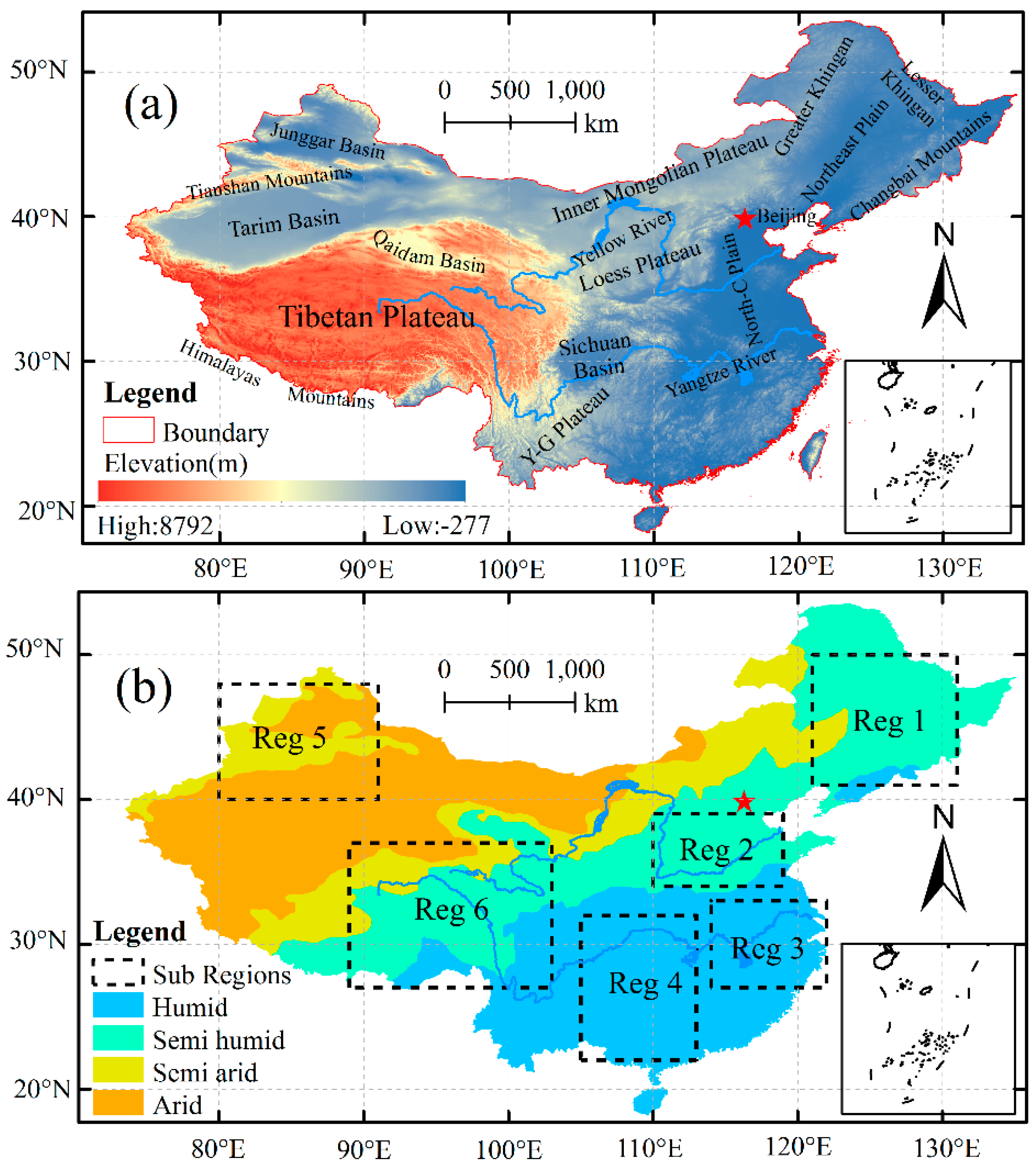
2.1. Study Areas

The study area is the entirety of mainland China located between 73°–135°E and 18°–53°N. The geography of China is variable, with regional differences in topography. The topographic variability described by the digital elevation model (DEM) from the Geospatial Data Cloud (http://www.gscloud.cn) is given in Figure 1a. From it, the terrain of China is gradually reduced from the northwest to the east, and can be broadly divided into three elevation belts: the first belt is the Tibetan Plateau, whose average altitude is above 4500 m; the second belt includes central and northern China, with an average elevation between 1000 m and 2000 m; and the third belt is mainly located in eastern China, with an average elevation of less than 500 m. The first belt is known as “the roof of the world”, and contains many star-studded mountains and glaciers. Moreover, the Qaidam Basin, whose average altitude is below 2000 m, is also within the first belt. There are many plateaus and basins scattered on the second ladder, including the Inner Mongolia, Loess, and Yunnan–Guizhou plateaus, and the Tarim, Junggar, and Sichuan basins. The third belt is dominated by hills, low mountains, and plains. The three major plains of China, namely, the Northeast, the North, and the Middle-Lower Yangtze plains, are all on the third belt.

China is located in the typical Asian monsoon region where the monsoon circulation plays an important role in the transportation of water vapor, and the path, source, and sink of water vapor transport determine the distribution of precipitation. Coupled with the effects of complex terrains, mainland China can be divided into four climate districts based on the spatial distribution of average annual precipitation [22]. The spatial distribution of the four climatic zones is shown in Figure 1b. It is obvious that a dry climate generally dominates vast areas of northwestern China, except for the Tianshan Mountains, where there is higher precipitation accumulation than the surrounding areas. Meanwhile, the southeastern part of China is mainly controlled by the humid climate, benefitting from the influence of the subtropical and tropical monsoons. For regional analysis, six subregions are selected based on Tang et al. [17]. Regions 1–2 are located in the semi-humid climate zone in northeast China, which is primarily controlled by the monsoon climate of medium latitudes and characterized by hot and wet summers and cold and dry winters [23]. Regions 3–4 are in the moist area of southern China, with hot and wet summers and a mild and dry intensity in winter. Region 5 is dominated by the temperate continental climate, with its little precipitation evenly distributed throughout the year [24]. Region 6 is situated across the transition from wet to dry, and is dictated by the plateau mountain climate. This region is characterized by complex topography and high elevation, and exhibits great precipitation spatial variability [25].

2.2. Ground Reference Data

The ground reference data is an hourly gauge-satellite merged product obtained from the CMDSC (http://data.cma.cn). This data set is produced by merging the ground data from more than 30,000 automatic weather stations (AWSs) over China with the CMORPH product by an improved probability density function–optimal interpolation method (PDF–OI) [26]. The entire process for generating the merged data requires four steps, which include: (1) interpolating the hourly AWSs’ observations with strict quality control onto regular grid points with a spatial resolution of 0.1° over mainland China using a modified climatology-based optimal interpolation (OI) algorithm [27,28,29]; (2) obtaining the CMORPH precipitation estimates (the original spatiotemporal resolutions are 8 km and 30 min, respectively), accumulating to an hourly rate and resampling onto a horizontal resolution of 0.1°; (3) correcting the hourly CMORPH by matching its probability density function (PDF) with the gauge precipitation analysis [29]; and (4) merging the bias-corrected CMORPH precipitation with the gauge-based analysis to generate the hourly merged precipitation product with a horizontal resolution of 0.1°. It turned out that the monthly spatial distribution of the merged product was similar to that of the China gauge-based daily precipitation analysis based on approximately 2400 national stations [26]. Moreover, the merged product performs reasonably well in China, and can capture the varying features of hourly precipitation in heavy weather events [30]. Furthermore, the merged product has already been used as reference data in the evaluation of GSPEs [20,31]. Therefore, we believe that the merged product can act as a benchmark for evaluating GSPEs. However, most of the hourly AWSs are located in southern and eastern China, and a relatively sparse gauge network exists across the northern and western parts, especially over the Tibetan Plateau. Thus, uncertainty still exists in the merged data, especially for sparse gauge areas, and could be a source of error in the evaluation of GSPEs in such regions [32]. Given that, the six selected subregions all have relatively high densities of gauges. Note that the assessment is performed at a 3-h temporal scale, so the reference data is summed up from hourly to the 3-h scale.

2.3. Satellite-Based Precipitation Products

For the primary objectives mentioned above, four GSPEs—namely, V05UC, V05C, V04C, and GSMaP—are used in this paper from April 2014 to December 2016. The four GSPEs are first accumulated to a 3-h scale to match the reference. Then, they are respectively grouped with the reference for further evaluation. Furthermore, the comparison of performance between V05UC and V05C can help quantify the improvement of the gauge calibration algorithm (GCA) used in V05C, and the difference between V05C and V04C can help accurately posit the promotion of the latest version. Meanwhile, the addition of GSMaP helps the subsequent analysis to be more rational and persuasive. The following is a brief introduction to the used GSPEs.

2.3.1. IMERG Products

The IMERG algorithm providing the multi-satellite precipitation products has been developed as a unified US algorithm, drawing on strengths from TMPA, PERSIANN-CSS, and CMORPH-KF. To obtain high spatiotemporal resolution precipitation estimations, the IMERG algorithm collects observations from the passive microwave (PMW) sensors flying on a series of satellites in low earth orbits (LEO) and the infrared (IR) sensors equipped in geosynchronous orbit (GEO) satellites. Given that the PMW provide intermittent but relatively accurate estimations by directly sensing rainfall, while the IR sensors provide excellent temporal resolutions but have great uncertainty caused by the indirect relationship with precipitation [33], the IMERG algorithm is designed to use as many PMW estimations as possible and fill in gaps with GEO-IR estimations. For this purpose, the PMW estimations are gridded, intercalibrated, and morphed, following the GEO-IR-based feature motion, and integrated by the GEO-IR estimations from PERSIANN-CCS when the PMW estimates are too sparse. Then, the monthly gauge precipitation data from the Global Precipitation Climatology Center (GPCC) Monitoring Product are introduced to provide crucial regionalization and bias calibration to the satellite estimates. More detailed information regarding IMERG can be obtained from the “IMERG Algorithm Theoretical Basis Document” [34] and the technical document that is accessible in Huffman et al. [35].

IMERG provides three types of products: early-run, late-run, and final-run products with spatial and temporal resolutions of 0.1° and 30 min, respectively, among which the early-run and late-run products are near real-time, with latencies of 4 h and 12 h, respectively, while the final-run product is a post real-time research product with a latency of approximately 2.5 months. Compared with the early and late products, the final products, as the research-level products, provide the uncalibrated and gauge-calibrated multi-satellite precipitation information. The difference between them is that the monthly gauge data set from GPCC is introduced into the bias-calibration algorithm for calibrated estimation, but not for the uncalibrated one. As noted above, the algorithm of IMERG has now been upgraded to V05, and the final-run IMERG are available as of November 2017. Similarly to the previous versions, the data record begins on 12 March 2014. The main changes from V04 to V05 are as follows: (1) the Goddard Profiling Algorithm (GPROF) that is used for computing precipitation estimates from all of the PMW sensors onboard GPM satellites has been updated from GPROF V04 to GPROF V05; (2) the high quality (HQ) precipitation field spatial coverage has been increased from 60° N–S to 90° N–S; (3) a Quality Index has been added for all of the 0.5-h and monthly products; and (4) gauge error estimates are refined to provide proper weighting when combined with satellite-only estimates. Detailed information on this conversion can be found in the V05 IMERG Final Run Release Notes [36]. Although, given the main objectives of this study, just three final-run IMERG products are employed in this paper, the near real-time IMERG products, including early-run and late-run products, also need to be assessed, given their widespread application in hydrometeorological modeling and disaster forecasting [37]. Future researches investigating this aspect should be recommended.

2.3.2. GSMaP Product

The GSMaP project [38] was originally sponsored by the Japan Science Technology Agency (JST) and is now sponsored by the Japan Aerospace Exploration Agency (JAXA). Since the GPM mission was launched, the GSMap project has released corresponding GPM-era precipitation products, namely, GSMap V6, by adding information from GPM Core GMI. In this version, the precipitation estimates were generated by the following three steps [39]: (1) calculating the rainfall rate from PWM sensors; (2) propagating the rainfall-affected area using forward and backward morphing techniques [40]; and (3) refining the estimated data based on infrared brightness temperature by a Kalman filter approach [41]. In the latest GSMaP V7 released in January 2017, some changes have been made to improve their performance, such as the DPR observations from the GPM-CO satellite being used as a database to improve the GSMaP algorithm, the snowfall estimation method and the NOAA multisensor snow/ice cover maps being implemented to improve the accuracy of precipitation estimation in the high latitudes, and the gauge calibration method and orographic rain calibration method having been improved. In this paper, the GSMaP_Gau (hereafter referred to as GSMaP) produced from GSMap_MVK and adjusted by the CPC global daily gauge data analysis [27] is employed.

3. Methods

To quantitatively evaluate the overall performance of the four GSPEs, a set of widely used traditional statistical metrics were adopted. Then, an error decomposition technique and the corresponding categorical statistical indices were applied to trace the sources of the errors in the GSPEs.

3.1. Continuous Statistical Indices

Two categories of statistical metrics were selected to comprehensively evaluate GSPEs. The first category includes the correlation coefficient (CC), describing the degree of linear correlation between the GSPEs and gauge observations. The second category includes the root mean square error (RMSE), the mean absolute error (MAE), and the relative bias (Rbias), which are used to describe the error and bias of GSPEs compared with gauge observations. Formulas and perfect values of those indices are listed in

Table 1. List of the continuous statistical indices used to compare the Global Precipitation Measurement (GPM)-era satellite-based precipitation estimations (GSPEs) and the gauged observations.

Statistic Metrics	Equation	Unit	Rang	Perfect Value
Correlation Coefficient (CC)	$\mathrm{CC}=\frac{{\displaystyle {\sum }_{i=1}^n(R_{o,i}-\overline{R_o})(R_{s,i}-\overline{R_s})}}{\sqrt{{\displaystyle {\sum }_{i=1}^n{(R_{o,i}-\overline{R_o})}^2}}\sqrt{{\displaystyle {\sum }_{i=1}^n{(R_{s,i}-\overline{R_s})}^2}}}$	NA	0~1	1
Root Mean Square Error (RMSE)	$\mathrm{RMSE}=\sqrt{\frac{1}{n}{\displaystyle {\sum }_{i=1}^n{(R_{s,i}-R_{o,i})}^2}}$	mm	0~+∞	0
Relative bias (Rbias)	$\mathrm{Rbias}=\frac{{\displaystyle {\sum }_{i=1}^n(R_{o,i}-R_{s,i})}}{{\displaystyle {\sum }_{i=1}^n{R}_{o,i}}}\times 100\%$	%	−∞~+∞	0
Mean Absolute Error (MAE)	$\mathrm{MAE}=\frac{1}{n}{\displaystyle {\sum }_{i=1}^n\left|R_{s,i}-R_{o,i}\right|}$	mm	0~+∞	0

Notation: $n$ represents the number of samples; $R_{s,i}$ and $R_{o,i}$ are GSPEs and gauged observations, respectively; $\overline{R_o}$ and $\overline{R_s}$ are the mean values of the corresponding elements.

.

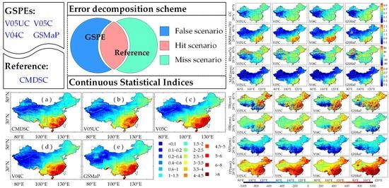
3.2. Error Decomposition

In this study, the simple and effective error decomposition scheme proposed by Tian et al. [19] and extended by Yong et al. [22] has been adopted and applied to trace the source of the errors in the four GSPEs. Through this method, the total precipitation bias (hereafter referred to as TB) can be decomposed into three independent components: hit bias (HB), missed precipitation (MP), and false precipitation (FP). The detailed concepts of the hit, missed, and false scenarios for the selected GSPE against the gauged observations are expressed in

Table 2. Contingency table showing how three independent error components (hit, missed, and false) are identified by dichotomous variables (satellite products and ground reference).

		Satellite Products
		Rain: 1	No rain: 0
Gauged Observations	Rain: 1	Hit	Missed
	No rain: 0	False	0

, in which a hit scenario represents GSPE and gauged observation reporting precipitation events simultaneously, a missed scenario shows that the precipitation signal is missed by GSPE but detected by gauged observation, and a false scenario indicates the opposite case of a missed scenario. In practice, two simple binary values (i.e., 1 and 0) can be used to identify raining and not-raining for GSPEs and gauged observations, respectively. According to this design, a binary mask and its Boolean complement are employed by Tian et al. [19] to divide the three error components. Given a precipitation field, $R(\overrightarrow{x},t)$, one can derive a binary-valued raining mask, $P(\overrightarrow{x},t)$, as follows:

$$P(\overrightarrow{x},t)=\{\begin{array}{cc}1\hfill & \mathrm{if}R(\overrightarrow{x},t)>0\hfill \\ 0\hfill & \mathrm{if}R(\overrightarrow{x},t)=0\mathrm{or}\mathrm{missing}\hfill \end{array}.$$

(1)

In reality, a small value (e.g., 0.3 mm/3 h) instead of 0 is usually used as the rain/no-rain threshold to determine the mask. Then, the respective event masks of the GSPE ($R_s(\overrightarrow{x},t)$) and the gauged observation ($R_o(\overrightarrow{x},t)$) can be performed using Equation (1). Subsequently, the hit mask ($P_{s,o}$), the missed mask ($P_{s,\overline{o}}$), and the false mask ($P_{\overline{s},o}$) for the chosen GSPE against gauged observation can be defined as:

$$\{\begin{array}{l}{P}_{s,o}=P_s\times P_o\\ P_{s,\overline{o}}=P_s\times P_{\overline{o}}\\ P_{\overline{s},o}=P_{\overline{s}}\times P_o\end{array};$$

(2)

where $P_s$ and $P_o$ denote the binary precipitation masks for the corresponding $R_s(\overrightarrow{x},t)$ and $R_o(\overrightarrow{x},t)$, and $P_{\overline{s}}$ and $P_{\overline{o}}$ are the Boolean complements of the corresponding elements. Here, the TB is defined as the difference between GSPE and gauged observation:

$$\mathrm{TB}=R_s-R_o.$$

(3)

Then, the HB, MP, and FP are defined following Tian et al. [19]:

$$\{\begin{array}{l}\mathrm{HB}=\mathrm{TB}\times P_{s,o}\\ \mathrm{MP}=R_o\times P_{s,\overline{o}}\\ \mathrm{FP}=R_s\times P_{\overline{s},o}\end{array}.$$

(4)

According to the derivation of Tian et al. [19], the relation between the three independent error components and the TB can be expressed as:

$$\mathrm{TB}=\mathrm{HB}-\mathrm{MP}+\mathrm{FP}.$$

(5)

Significantly, TB, HB, MP and FP still contain spatial and temporal information, and the relation described in Equation (5) still holds when spatial and temporal averaging is applied. Meanwhile, because the three individual components make variable contributions to TB (e.g., MP and FP always generate opposite biases, canceling each other out, and HB could be positive or negative for hit scenarios), the three individual components could have larger amplitudes than TB. This indicates that the TB employment by most conventional studies is not enough to truly understand the error features of GSPEs. In addition, to better trace the error source and understand the error structure contained in GSPEs, three categorical statistical indices, including FAR (false alarm ratio), POD (probability of detection) and CSI (critical success index), are also adopted in this paper. Their detailed descriptions are as follows:

$$\{\begin{array}{l}\mathrm{FAR}={\displaystyle {\sum }_1^k{P}_{\overline{s},o}}/{\displaystyle {\sum }_1^k{P}_o}\\ \mathrm{POD}={\displaystyle {\sum }_1^k{P}_{s,o}}/{\displaystyle {\sum }_1^k{P}_s}\\ \mathrm{CSI}={\displaystyle {\sum }_1^k{P}_{s,o}}/{\displaystyle {\sum }_1^k(P_{s,o}+P_{s,\overline{o}}+P_{\overline{s},o})}\end{array}.$$

(6)

where k represents the number of time samples. Actually, POD gives the fraction of hit events among all of the actual precipitation events, and FAR gives the fraction of false events among all of the events detected by GSPEs. CSI is a more balanced index, combining the characteristics of false alarms and missed events, and can be expressed as a function of POD and FAR [17]. In practice, the categorical statistical indices FAR, POD, and CSI are very effective in assessing rain area delineation and raining or not-raining detection, while the error decomposition scheme is a quantitative assessment for hit, missed, and false scenarios.

4. Results

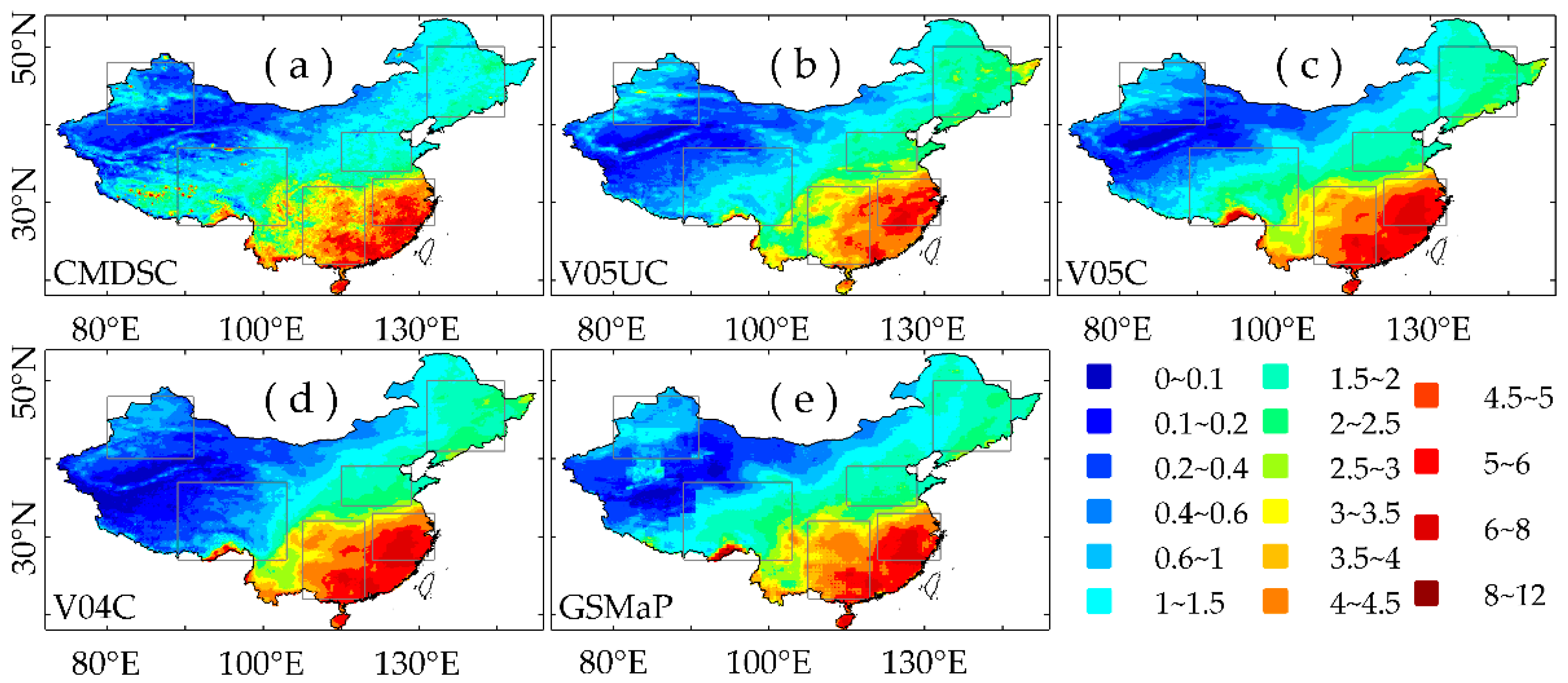
4.1. Spatiotemporal Analyses of Precipitation Accumulation

To analyze the accuracy in capturing precipitation accumulation between April 2014 and December 2016, the spatial distributions of daily average precipitation derived from CMDSC and GSPEs are illustrated in Figure 2 at 0.1° × 0.1° resolution. Intuitively, the spatial patterns of the GSPEs shown in Figure 2 are visually compatible with CMDSC, which means that the four GSPEs can generally capture the spatial patterns of precipitation accumulation over mainland China. Even so, differences between disparate products or multiple versions still exist. For instance, the calibrated V04C, compared to other estimations, shows obvious underestimates in the Tibetan Plateau, but holds a higher level over southeast China, while V05UC has the lowest precipitation of the multiple GSPEs over southeast China. In addition, from the CMDSC (Figure 2a), it is notable that the precipitation shows strong spatial heterogeneity, with the precipitation intensities gradually decreasing from the southeast to the northwest and northeast. Meanwhile, the highest precipitation is concentrated on the southeast coast, while the lowest precipitation appears in the Tarim Basin. Considering the regional difference, there is a need to subdivide national-scale analyses into regional components.

Daily average precipitations from four GSPEs within the six regions of mainland China during April 2014 and December 2016 have been plotted in Figure 3 versus the CMDSC. The corresponding quantitative indices, including the CC, Rbias, and RMSE computed from all of the records within the corresponding region, are also added in Figure 3. The figure clearly shows that all four GSPEs exhibit serious overestimation in regions 1–2 with relatively high positive Rbiases (31.24%, 28.87%, 25.31% and 21.16% for Region 1, and 37.09%, 25.52%, 25.84% and 23.41% for Region 2). This overrated pattern is primarily due to ice or snow cover and the high latitude, which complicate satellite observations [42]. Note that, although the overrated situation is not effectively assuaged, the CCs and RMSEs of V05C, VO4C, and GSMaP are significantly improved by gauge calibration, indicating that gauge calibration is beneficial for acquiring more accurate precipitation distributions in cold regions. In summary, GSMaP is the best of the four GSPEs in regions 1–2, with the highest CCs (0.76 for Region 1 and 0.75 for Region 2), and the lowest Rbiases (21.16% for Region 1 and 23.41% for Region 2) and RMSEs (0.37 mm for Region 1 and 0.41 mm for Region 2).

In regard to the low-latitude and moist aspects of regions 3–4, all four GSPEs perform better than in regions 1–2. The performance boost of the four GSPEs over regions 3–4 mostly benefits from the relatively flat terrain and humid climate, which suit satellite observations. Furthermore, the differences between uncalibrated V05UC and the three calibrated products (V05C, V04C, and GSMaP) are remarkable. V05UC has the best Rbiases (6.42% versus 16.91%, 16.12%, and 13.40% for Region 3, and 6.99% versus 11.31%, 12.71% and 8.81% for Region 4), but also the worst CCs (0.73 versus 0.85, 0.84 and 0.85 for Region 3, and 0.66 versus 0.83, 0.81 and 0.85 for Region 4). Moreover, the gauge calibration algorithms used in V05C, V04C, and GSMaP all tend to increase precipitation accumulation over high-precipitation regions (daily average precipitation higher than four mm/day) and thus lead to greater Rbiases. Therefore, the three calibrated products do not show sufficient advantages in Rbias and RMSE in spite of the improvements in CC within regions 3–4.

As for Region 5, which is characterized by an arid climate, the uncalibrated V05UC shows significant overestimation, with an Rbias over 30%. This is not surprising, since hydrometeors detected by the spaceborne sensors (which generally sample from the ice phase or cloud tops) may partially or totally evaporate before they reach the surface due to the strong evaporation. Although the Rbias appears to be effectively controlled in V05C, V04C, and GSMaP (11.12%, 12.76% and 21.75% versus 30.62%, respectively), because the CCs (0.5, 0.33 and 0.47 versus 0.47, respectively) and RMSEs (0.41 mm, 0.44 mm and 0.43 mm versus 0.48 mm, respectively) do not have remarkable improvements, they all struggle in capturing accurate spatial precipitation accumulations. Hence, the application of the four GSPEs over Region 5 should be used with caution. Besides, some high-precipitation grid cells (above 2 mm/day) are found in uncalibrated V05UC, but they are not detected by the calibrated products (V05C, V04C, and GSMaP). The primary reason is that the ground-based observations used in IMERG and GSMaP have not detected these high-precipitation areas, and thus remove these outliers via the gauge calibration algorithm.

Most parts of Region 6 are located within the Tibetan Plateau and sit astride the transition zone from a humid area to an arid area. Although the bias-adjusted process corrected the notable underestimation of V05UC, with the Rbiases improving from −35.53% to 3.89%, many points of the calibrated V05C still scatter far from the 1:1 reference line and present polarization features. This indicates that some inner subregions of Region 6 still exhibit extreme overestimated or underestimated scenarios. The basin-scale or finer subregion analyses are needed to locate the error. Meanwhile, the CC Rbiases contained in GSMsP are close to those in V05C with greater spatial heterogeneity. Furthermore, a severe underestimation (Rbias = −47.77%), which does not appear in IMERG inchoate versions [17], is displayed in V04C. Fortunately, this underestimation has been suppressed in the latest calibrated version. This situation should be borne in mind for IMERG users dealing with the Tibetan Plateau. Besides, Region 6 shows the most dispersed graphs among the six subregions. Several factors could contribute to these distributed graphs: (1) the topography and climate over this region are complex, posing a great challenge for remote sensing observations; (2) the performance of current retrieval algorithms is limited in catching the warm rain processes or short-lived convective storms caused by topography and climate over this region; (3) few gauges are used in the gauge calibration algorithm, which potentially degrades the quality of these GSPEs.

In general, compared to the satellite-only product (V05UC), the bias-corrected products have a positive correction over regions 1–4. However, the overestimation of precipitation still cannot be ignored, especially for regions 1–2, where the containing Rbiases are above 20%. Similarly, with a slight performance improvement, the expected quality improvements do not appear in the IMERG product update (from IMERG V04 to V05) over the above regions. It may benefit from the addition of the IR streams that slightly improved the relative balance, and the performance of GSMaP is faintly superior to the three IMERG products based on the CCs, Rbiases, and RMSEs over regions 1–4. The application of the four GSPEs should be used with caution over Region 5 given the struggling performance in obtaining accurate precipitation accumulation. For stable results, more sophisticated segmentation is required over Region 6.

To check the consistency of the precipitation in the time series, the 3-h timescale regional averaged precipitation accumulations from the four selected GSPEs versus the CMDSC are scattered in Figure 4. Meanwhile, the Quantile–Quantile (Q–Q) plot technique is also adopted to illustrate more insight into the natural differences between the four GSPEs and the CMDSC over the six regions of mainland China. It is well known that if the GSPEs are close to the observed ones, the points in the Q–Q plots (green) should fall close to the 1:1 reference line (blue lines). The greater the departure from the reference line or the nonlinearity of the resulting graph, the greater the evidence of heterogeneity [43]. It is evident that, despite the slight overestimation in high-precipitation events, the performances of GSMaP are remarkably better than those of the other three GSPEs over regions 1–4. Additionally, in each corresponding region of regions 1–4, GSMaP possesses the best CC and RMSE. Meanwhile, in Region 1 and regions 3–4, the two calibrated IMERG products (V05C and V04C) display slight improvements relative to the uncalibrated product (V05UC), but do not effectively inhibit the overestimation of heavy precipitation. In Region 2, the uncalibrated V05UC tends to overestimate the moderate precipitation (3–6 mm/3 h), but underestimate the heavy rainfall (more than 6 mm/3 h). Note that this overestimation and underestimation have been effectively controlled in its calibrated version, V05C. In general, with high CCs, the four GSPEs better delineate the regional average precipitation process in the 3-h timescale over regions 1–4. However, the abilities of the four GSPEs in depicting 3-h-scale regional averaged precipitation accumulation are significantly reduced in regions 5–6. In these two regions, V05C exhibits a slight advantage, but the undulate properties in high-precipitation events (underestimation in Region 5 but overestimation in Region 6) demonstrate that there is much room for improvement.

4.2. Spatial Statistical Analysis

Spatial distributions of continuous statistical indices for the chosen four GSPEs at 3-h and 0.1° × 0.1° resolution over mainland China are shown in Figure 5. From it, the spatial distributions of CCs are positively correlated with precipitation accumulations (Figure 1b and Figure 2). In humid and semi-humid regions, the CCs oscillate approximately 0.6. However, they get lower in semi-arid and arid regions, particularly for the Tarim Basin and northern Tibetan Plateau, where the CCs are mainly under 0.2. The main causes of this situation are the interferences of complex topography and climate, which pose a great challenge for accurate satellite precipitation estimation [44]. Meanwhile, a limited number of gauges are adopted by the GPCC monthly gauge or CPC global daily gauge data analysis over such areas, thus generating a potential performance reduction compared to the other regions. Furthermore, the deterioration of CMDSC data is also a reason behind the reduced reliability of statistical indices. The RMSEs and MAEs also show similar spatial distributions to that of precipitation accumulations. This indicates that RMSEs and MAEs are closely interrelated for precipitation accumulation. Moreover, despite the prominent underestimation of V04C over the entire Tibetan Plateau, the GSPEs are all better or slightly overestimate the precipitation in east and south China, and significantly underestimate the precipitation in the northern Tibetan Plateau. In addition, all four GSPEs extremely overestimate the precipitation over northwestern mainland China, especially for GSMaP in the Tarim Basin, where the Rbias is above 80%.

Figure 6 shows vertical error bars (±σ) of continuous statistical indices for the chosen four GSPEs at a 3-h timescale over the six selected regions. The contrast of CCs (Figure 6a) and Rbiases (Figure 6c) between the six regions proves that all four GSPEs show better performance in regions 1–4 than that over regions 5–6. Meanwhile, the stable property is approved over regions 1–4, while strong spatial heterogeneity is contained in the GSPEs over regions 5–6. This phenomenon is reasonable, because regions 1–4 have greater precipitation intensities and relatively flatter topography than regions 5–6, which is beneficial to precipitation estimation. Since the RMSE and MAE vary greatly over the six regions due to the heterogeneity of precipitation accumulation, they are not suitable to be compared between multiple regions. However, for each of the six regions, the comprehensive consideration of four statistical indices can effectively provide advice on which one of the four GSPEs is most suitable. Compared to the three IMERG-based products, GSMaP has a slight advantage over regions 1–4, but shows steep regression over regions 5–6. Of the three IMERG-based products, V05C is the best in the statistical analysis, but the minor improvements have not resulted in a qualitative upgrade in quality. This result is consistent with the above analysis in Section 4.1. Besides, although all four GSPEs have relatively finer spatial resolution (0.1°), given the greater spatial heterogeneity of precipitation in complex terrain, the spatial resolution of these GSPEs is still too coarse to resolve the mountain valley precipitation contrasts in complex topography where the terrain varies considerably. This may be one of the reasons why GSPEs performed poorer in regions 5–6 than in regions 1–4. The quantitative precipitation estimations from regional kilometer-scale climate modeling are really promising in complex terrains, especially for extreme storm events. How to select the optimal precipitation data source will be an important topic for disaster forecasting (e.g., floods and mudslides) in such areas.

4.3. Error Components Analysis

Figure 7 displays the spatial distribution of the error components that were each accumulated for the entire study period from April 2014 to December 2016. Meanwhile, the spatial distributions of corresponding categorical statistical indices (FAR, POD, and CSI) are illustrated in Figure 8. It is very evident from Figure 8 that the spatial distributions of FAR, POD, and CSI for V05UC and V05C are identical. This indicates that the GCA calibration used in V05C cannot change the rain area delineation and raining or not-raining detection, and further results in the MPs of V05UC and V05C in Figure 7 exhibiting the same spatial distribution. Since gauge calibration is mainly focused on rain signals determined by GSPEs, this failure in MP is understandable. Moreover, the amplitude of TB for V05C is slightly less than that for V05C over northeast China (e.g., regions 1–2), indicating a slight improvement in V05C. Further analysis indicates that this improvement is mainly attributed to the reduction of FP and HB via GCA calibration in these regions. Moreover, one can see that V05UC systematically underestimates the precipitation over most parts of south China and the Tibetan Plateau (regions 3–4 and Region 6 as examples), while an opposite overestimation occurred in V05C. This shows that the upward adjustment of the GCA calibration can alleviate the underestimation that occurred in the uncalibrated V05UC over south China and the Tibetan Plateau, but meanwhile, the amplitude of the FP is also magnified. The most notable difference between the two calibrated IMERG products (V05C and V04C) occurs in the eastern Tibetan Plateau. V04C shows an extreme underestimation over the eastern Tibetan Plateau, but mainly because of the elevated POD and the upward adjustment of the latest GCA calibration, and this underestimation is effectively alleviated in V05C. In addition to the southern Tibetan Plateau, the error components as well as categorical statistical indices of V04C are almost identical to V05C, which indicates that the performance of V05C is not substantially improved over most of mainland China. Nevertheless, due to the lack of accurate precipitation, the performance improvement of V05C on the southern Tibetan Plateau is still exhilarating.

Although the spatial distribution of TB is similar, the error components of GSMaP are a far cry from those of V05C. For southern China, GSMaP has the best POD and CSI, but also the worst FAR (Figure 8). We speculate that this can mostly be attributed to overestimation in precipitation occurrence probability. It is also why GSMaP contains the largest FP and lowest MP over southern China (Figure 7). Moreover, GSMaP shows a remarkable negative HB over southern China, which leads to underestimation, but the amplitude is much less than the corresponding FP. Therefore, GSMaP has slightly overestimated precipitation in southern China, which is similar to V05C. With regard to northeast China, GSMaP has similar MP and FP values to the IMERG products, but contains a lower HB. Hence, the better TB is monitored in GSMaP over northeast China, whereas abrupt FP appears in GSMaP over northwest China, particularly in the Tarim Basin, resulting in the poor performance of GSMaP over these regions.

In general, the largest FPs of the four GSPEs are situated in low-latitude humid areas. Meanwhile, HB and MP also have the largest amplitudes in these regions. This may be related to the limitation of current satellite precipitation retrievals in catching the warm rain processes or short-lived convective storms [19]. In addition, although the error component is different, the four GSPEs all show limited performance in the Tibetan Plateau and Tianshan Mountains. This is possibly due to the perturbance of complex topography and arid climate. However, the reduced performance of the reference data is also a major reason.

To investigate the temporal variations of error components for the four GSPEs during the study period (from April 2014 to December 2016), a time series of regional averaged error components and TB are depicted in Figure 9 at a 3-h resolution. For smoothing and reducing visual clutter, a 10-day (80 samples at a 3-h scale) moving average was applied to the entire time series. Obviously, there exists an obvious seasonality in the error components, particularly for the summer and winter months. Generally, almost all of the error components and TB show higher values in the summer and lower ones in winter over the six regions. Such a significant season-driven error structure is primarily related to the uneven seasonal distribution of precipitation over China. Meanwhile, the changing tendency of error components and TB also shows remarkable regional differences.

In terms of uncalibrated V05UC, the changing tendency of HB generally agrees well with that of TB, while the amplitude of HB is relatively lower than TB. Over regions 1–2, the positive HB and FP are the main contributors to the TB of V05UC. For regions 3–4, as the proportion of MP increases, MP and FP tend to be symmetrical, such that their overestimation and underestimation may cancel each other out. As a result, the curves of HB are very close to those of TB over regions 3–4. Notably, HB is inclined to be negative in summer and positive in winter, and thus leads to a similar seasonal cycle of TB. With respect to Region 5, because the HB and MP are considerably smaller, the overestimation of total errors in V05UC is primarily from FP. For Region 6, it is quite obvious that the curve of the TB almost coincides with that of MP to cancel out the negative HB and positive FP.

In regard to the calibrated V05C, the most striking feature is the decrease of amplitude in HB and TB. However, as described above, the MP has barely improved. Moreover, the calibrated effect also has remarkable regional differences. Taking regions 3–4 as examples, one can see that the adjustment is mainly to increase the rain rates in summer rainy events and suppress the rain rates in the winter. Simultaneously, with the increase of summer rain rates, the FP in summer is also slightly strengthened. An opposite process takes place in Region 5; the overestimation caused by FP and HB has been effectively suppressed in summer, but in winter, the overestimation has a faint magnification. Compared to its successor V05C, V04C contains nearly the same error structure over regions 1–5. However, the excessive FP has resulted in the systematic underestimation over Region 6, and limits its application over these regions. Since the error components and the TB are all similar to that of the corresponding V05UC, the poor performance in Region 6 may be due to the failure of the calibration process. For GSMaP, the FP is the highest of the four selected GSPEs, and the MP is the lowest. Meanwhile, the HB of GSMaP usually behaves as negative numbers over the six regions, especially in summer months, which is not the same as the two calibrated IMERG products (V05C and V04C). Benefiting from the mutual melting of error components, the TB of GSMaP is usually the lowest over regions 1–4. However, the excessive FP still brings a potential pitfall in the application of hydrology.

4.4. Intensity Distribution Analysis

Accurate documentation of rainfall frequencies with different intensities plays the same important role with the average amount and spatiotemporal variation patterns of precipitation [42], because the same precipitation amount in the form of long-lasting light rain or a short-duration storm will yield quite different impacts in many aspects [28,45]. The PDFs of 3 h of precipitation accumulation for the four GSPEs and the gauged observation over six selected regions are shown in Figure 10. Since the PDFs are closer to lognormal than to Gaussian, the logarithmic scale is used to bin the precipitation rates across the range of 0.3–256 mm/3 h on the x-axis. The values on the y-axis stand for the proportion of precipitation accumulation for each bin in the corresponding total precipitation. Here, the threshold for rain or not-rain is 0.3 mm/3 h, but it may be slightly higher for the arid areas of Region 5 and Region 6 with complex climates. Research merely for these areas may require a smaller threshold.

The PDFs of both V05C and V05UC are generally similar to those of gauged observation over regions 1–4. This indicates that both V05C and V05UC show excellent capacity in capturing accurate PDFs over these regions, and that the calibration process used in V05C has not taken remarkable effect over regions 1–4. However, Region 5 is an exception, since the PDFs of both V05C and V05UC overdetect light and moderate precipitation events (rain rate <3 mm/3 h) and underdetect heavy precipitation events (rain rate >3 mm/3 h). Simultaneously, V05C does not show its advantages for a super performance in PDF match. In reality, the overestimation of light and moderate precipitation and the underestimation of heavy precipitation of V05C become even more pronounced over Region 5. This may be related to the arid climate condition and little gauge observation participating in the calibration procedures. The performance of V05UC in Region 6 is similar to that in Region 5, but the curve of V05C in Region 6 is very close to that of the CMDSC, which shows that the calibration process has been very effective for Region 6. With predominant overdetection of heavy precipitation events, the curves of V04C are far from the reference curves, particularly in regions 5–6, where the curves show extreme volatility. At this point, IMERG’s V05 values show a significant improvement from those of V04. As shown in Figure 10, the GSMaP overestimates light rain volumes (<6 mm/3 h for regions 1–4 and <2 mm/3 h for regions 5–6), but underestimates heavy rain volumes, which is quite different from the IMERG products over regions 1–4. In general, the calibrated V05C has the best performance for PDFs over selected regions. Meanwhile, the performance of the latest IMERG products (V05C and V05UC) is remarkably superior to V04C and GSMaP in capturing heavy precipitation, reflecting that the latest IMERG products can better reconstruct extreme events such as hurricanes [46].

To further understand the error features in various intensities, we computed the relative ratio of TB and its error components in the corresponding bin at a 3-h temporal resolution for the six selected regions during the study period (Figure 11). Obviously, the ratios of TB are probably lower than some of its error components. In fact, this is not surprising in GSPEs, owing to the mutual melting of the error components. For V05UC and V05C, the error features of FP and MP are very similar in that they both have large amplitudes at lower rain rates (<8 mm/3 h). Simultaneously, over northern China (regions 1–2 and Region 5), the amplitudes of FP are significantly higher than those of MP, while an opposite scenario has occurred in southern China. Meanwhile, the HBs are close to 0 or slightly positive values at lower rain rates in northern China, but they exhibit negative values in southern China. All of these factors lead to an overestimation for V05UC and V05C in northern China and an underestimation in southern China. With increasing precipitation density, the contributions of FP and MP decrease rapidly, but the amplitudes of HB increase dramatically, particularly for V05C in regions 3–4. Thus, the curves of TB in heavy precipitation events are closer to HB. Note that, compared to V05UC, although the FP and MP are not effectively controlled in Region 6, the amplitudes of HB and TB are greatly reduced. This could be the most symbolic improvement of V05C. For the anterior version, V04C, the distributions of FP and MP are very similar to V05UC and V05C over regions 1–4, but the amplitudes of TB and HB are much higher than the latest version in heavy precipitation events, showing a positive improvement. Moreover, the unstable FP, enhancive MP, and larger negative TB in regions 5–6 indicate that V04C has poor performance in these regions. Fortunately, this situation has been greatly improved in the latest version. For GSMaP, one can see that the distributions of TB have an evident tendency to overestimate lower precipitation rates (<8 mm/3 h for regions 1–4 and 3 mm/3 h for regions 5–6), and underestimate higher ones, which is a common error feature of satellite-based retrievals [47] caused by the nonunique relation between surface precipitation and brightness temperature [22]. Meanwhile, the curves of the TB are close to FP in lower precipitation rates, but close to HP in higher ones. This indicates that the primary contribution of TB is FP in lower precipitation rates, but turns to HP in higher ones, and further indicates that the gauge-adjusted process used in GSMaP does not effectively correct the HB contained in higher precipitation rates.

5. Discussion

Although GSPEs can provide finer spatial and temporal resolution for precipitation estimation with the implementation of a GPM mission, it can be inferred from the results of this study that they still present notable bias over some regions. Considering the spatial heterogeneity of precipitation and the complicated relations between surface precipitation and remote observations, efforts on GSPEs are still praiseworthy. However, as SPEs have done, the retrieval processes for both PMW and IR still contain two steps, namely, screening to detect raining and not-raining pixels and establishing the relationship between remote observations and surface rain rates for rainy pixels. Each step can contain errors, i.e., a missed error or false error may exist for the screening step and hit error for the other step. All of the errors can be spread through the applied integration processes. Conventional approaches for GSPEs assessment are directly compared against gauge data or ground-based radar estimates by using continuous statistical indices [15,17,18,31]. Guided by this principle, the overall performance of GSPEs can be investigated and quantitatively analyzed. Another way to assess GSPEs is based on their predictive ability of streamflow rate in a hydrological modeling framework [2,14]. Additionally, some researchers have combined the two approaches into a single study to comprehensively evaluate the performance of GSPEs [48,49]. Notably, these methods can provide the overall performance of GSPEs, but they all fail to locate where the retrieval errors are coming from. The error decomposition analysis introduced by Tian et al. [19] solves this problem by separating the total bias into three decompositions corresponding to the generation process. The integrated systems approach containing the continuous statistical indices and error decomposition analysis surely provides an in-depth exploration of the error structure, and thus provides deep guidance for algorithm developers or data users. However, because there are no records of the hydrological simulation of these GSPEs, further studies regarding their utility in hydrology and associated uncertainty analyses should be conducted. Moreover, the retrieval algorithms of GSPEs are usually optimized for particular regions [50], which could cause mild maladaptation for other regions. China has vast land, varieties of climates, and some unique terrains, but to our knowledge, there has been no evidence regarding the adjustment of GSPEs for mainland China thus far [20]. This may be one possible challenge for GSPEs in mainland China, particularly for northwest China and the Tibet Plateau, where GSPEs have room to further improve their capability. Besides, the diurnal cycle is one of the most important characteristics of precipitation, which is closely related to the formation mechanism of precipitation, but the diurnal cycle of precipitation in China shows remarkable regional discrepancy and seasonal variation. Although we have selected six typical subregions for in-depth analysis, the spatial heterogeneity of the diurnal cycle within these subregions is still strong. Therefore, we do not provide a performance evaluation for a diurnal cycle of precipitation in this paper; however, we highly recommend this aspect for future research studies that aim to assess satellite-based products over small or medium regions.

Since ground observation networks provide more accurate precipitation observations while SPEs have fine spatial and temporal coverage, the gauge combined or calibrated satellite-based precipitation estimation (termed as CSPE) is considered to be more advantageous in obtaining accurate regional precipitation estimation [2,51]. In this research, V05UC is a satellite-only precipitation estimation, and the other three are CSPEs, of which V05C and V04C were calibrated by GPCC at a monthly scale via GCA [9], and GSMaP was corrected by CPC global daily gauge data analysis via the GSMaP_Gauge algorithm (GGA) at a daily scale [52]. GCA and GGA may benefit from reducing the regional and seasonal TB contained in GSPEs, but they do not change the rain area delineation and raining or not-raining detection. Thus, the MP and FP contained in high-resolution CSPEs could not be alleviated [53]. This limitation may lead to various influences on the performance of these algorithms. For instance, the GCA used in IMERG was performed by creating a correction coefficient for each grid and each month, but it could not influence the MB, because the missed detected value was set to zero. Meanwhile, for some regions (i.e., the south part of mainland China), the multiplication of the correction coefficient enlarges the magnitude of the FP and thus offsets the improvement of the HB, reducing the performance of GCA. Similar results were also supported by the verification of IMERG over eastern China [20]. This phenomenon needs to be taken seriously.

Furthermore, GCA and GGA were operated on a global scale, but the global gauge network’s distribution used in GPCC or CPC is relatively sparse (i.e., only 194 of China’s International Exchange Stations (CIESs) were adopted by GPCC over the entirety of China [54]) for most regions, which further limits the performance of the calibration algorithm greatly. Since Sun et al. [51] indicated that regional-scale or national-scale modifications that employ more available rain gauge observations show great advantages in improving the quality of precipitation data, readjustment for each study area is an effective way to reduce errors before use in practical applications. Moreover, Su et al. [2] reiterated that fine time-scale modifications have an edge over coarseness, particularly for wickedly heavy precipitation. Note that GSMaP was adjusted in a finer time-scale than IMERG; this may be why GSMaP has slightly superior performance over regions 1–4 than IMERG. Additionally, the short latency time (one or two days) is also a significant advantage of GSMaP in comparison with the final-run IMERG’s two to four months.

In addition, it should be noted that the reference used in this paper is a gauge-satellite merged product produced by merging 30,000 AWS records and 8-km and 30-min resolution CMORPH estimation into a unified product via PDF–OI. Since the reference is not a truly independent reference, and the CMORPH approach is also used in the construction of IMERG, there might be some cross-correlated errors between the reference and IMERG, thus biasing the assessment result of IMERG. Even so, given the excellent performance in capturing the spatial and temporal distribution of precipitation, CMDAS has already been employed as the reference in assessing IMERG [31,55,56]. Further uncertainty analyses regarding these cross-correlated errors should be conducted. Moreover, it should be noted that the evaluation results for V04C are highly consistent with previous studies [21,55,57,58]. Furthermore, Omranian and Sharif [37] indicated that the performances of GSPEs are sensitive to changes in temporal and spatial resolution. However, the impacts of temporal and spatial downscaling or upscaling of these GSPEs on their accuracy are not studied in this paper. Therefore, more efforts are urgently needed to explore how these impacts work.

6. Conclusions

In this study, we comprehensively evaluated the quality of four GSPEs (i.e., V05UC, U05C, V04C, and GSMaP) over mainland China between April 2014 and December 2016 via continuous statistical indices against ground-based observations from CMDSC. In this process, their overall performances were quantified and cross-compared at national and regional scales. Then, the total biases (TBs) of these data sets were decomposed into three independent components, namely, hit bias (HB), missed precipitation (MP), and false precipitation (FP), based on Tian et al. [19]. In this manner, error sources and error characteristics were closely associated with the precipitation retrieval algorithms. The key findings are summarized as follows:

(1)

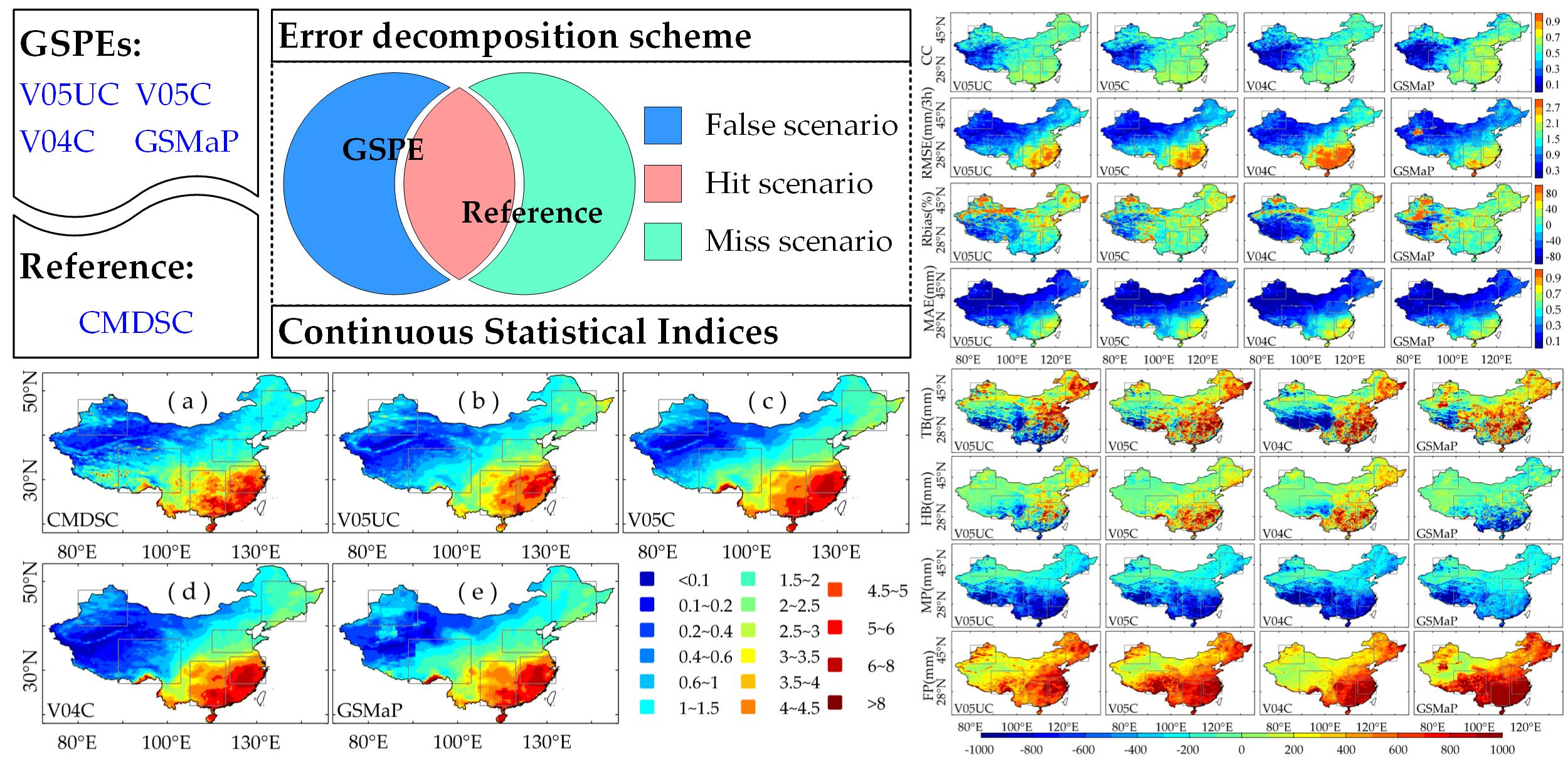
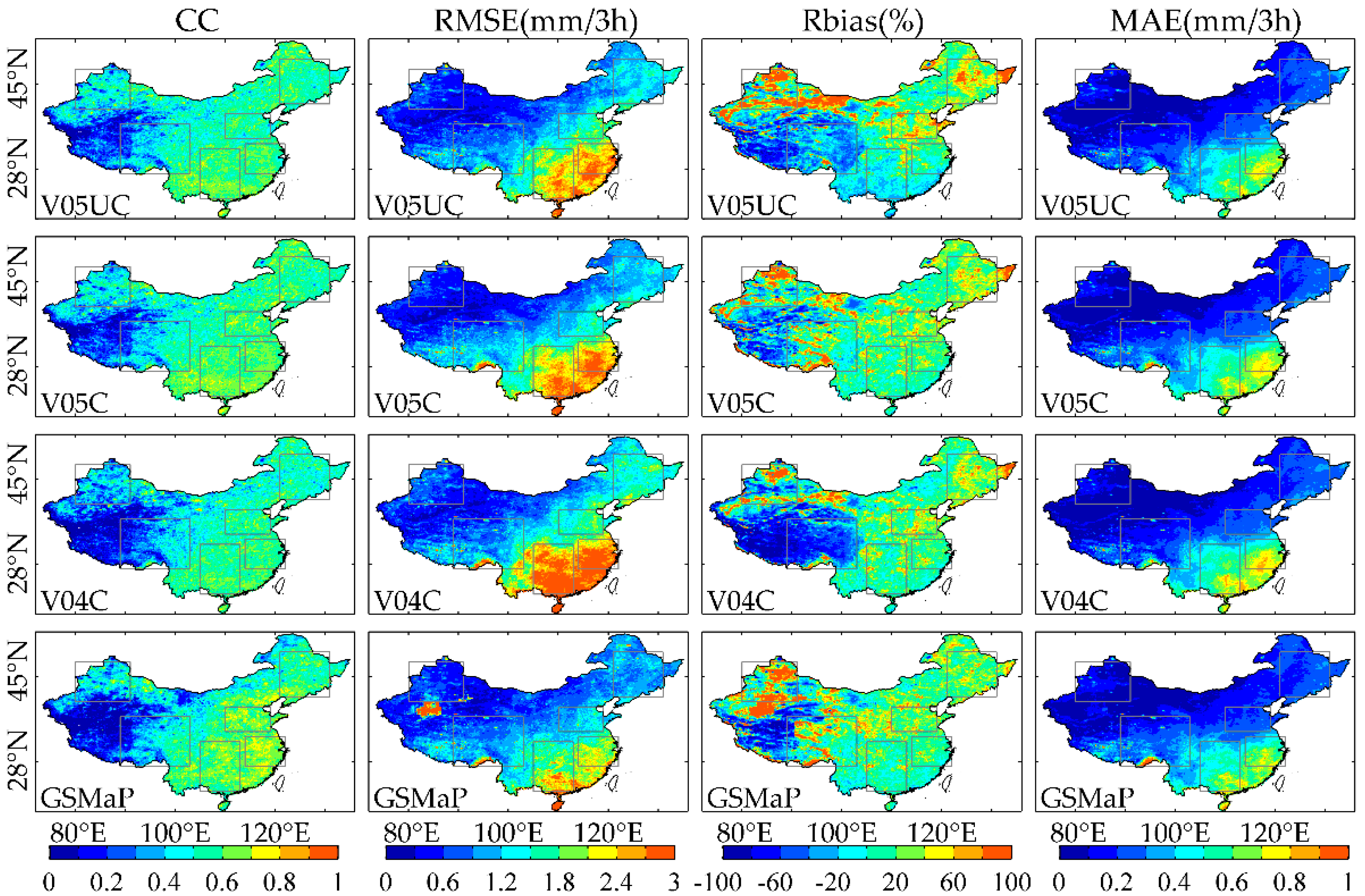
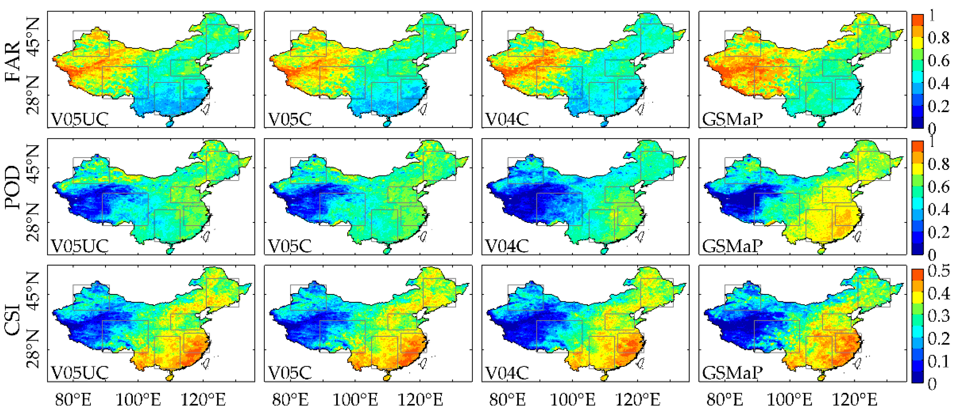
Compared to the CMDSC, the four GSPEs could generally capture the spatial patterns of precipitation over mainland China in spite of the overestimation in the southeast and the underestimation in the northern Tibetan Plateau. Overall, the quality of the four GSPEs in the humid and flat east was better than that in the arid and hypsographic west, with higher CCs of approximately 0.6 occurring in the east, but relatively lower CCs appearing in the west.

(2)

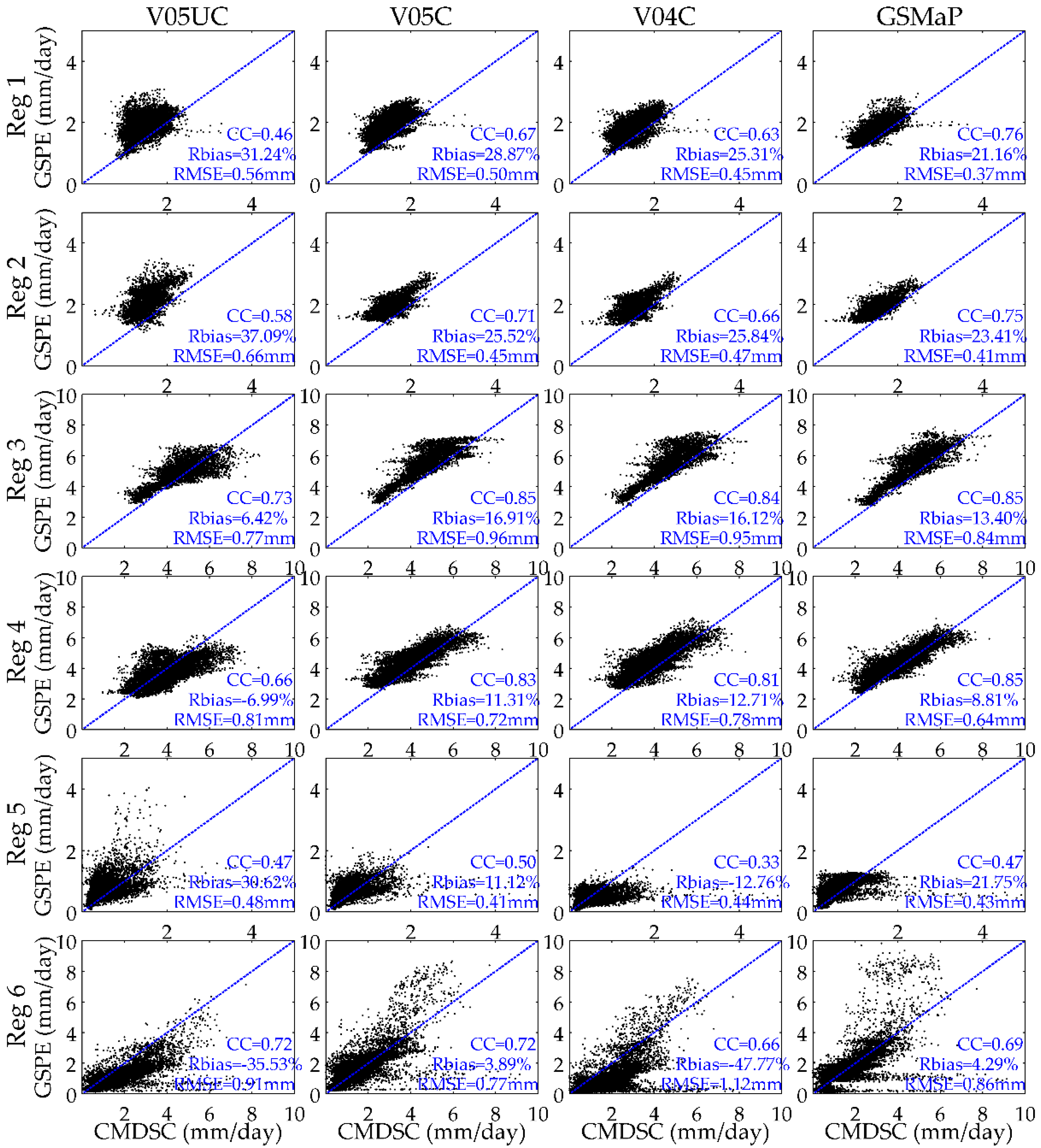
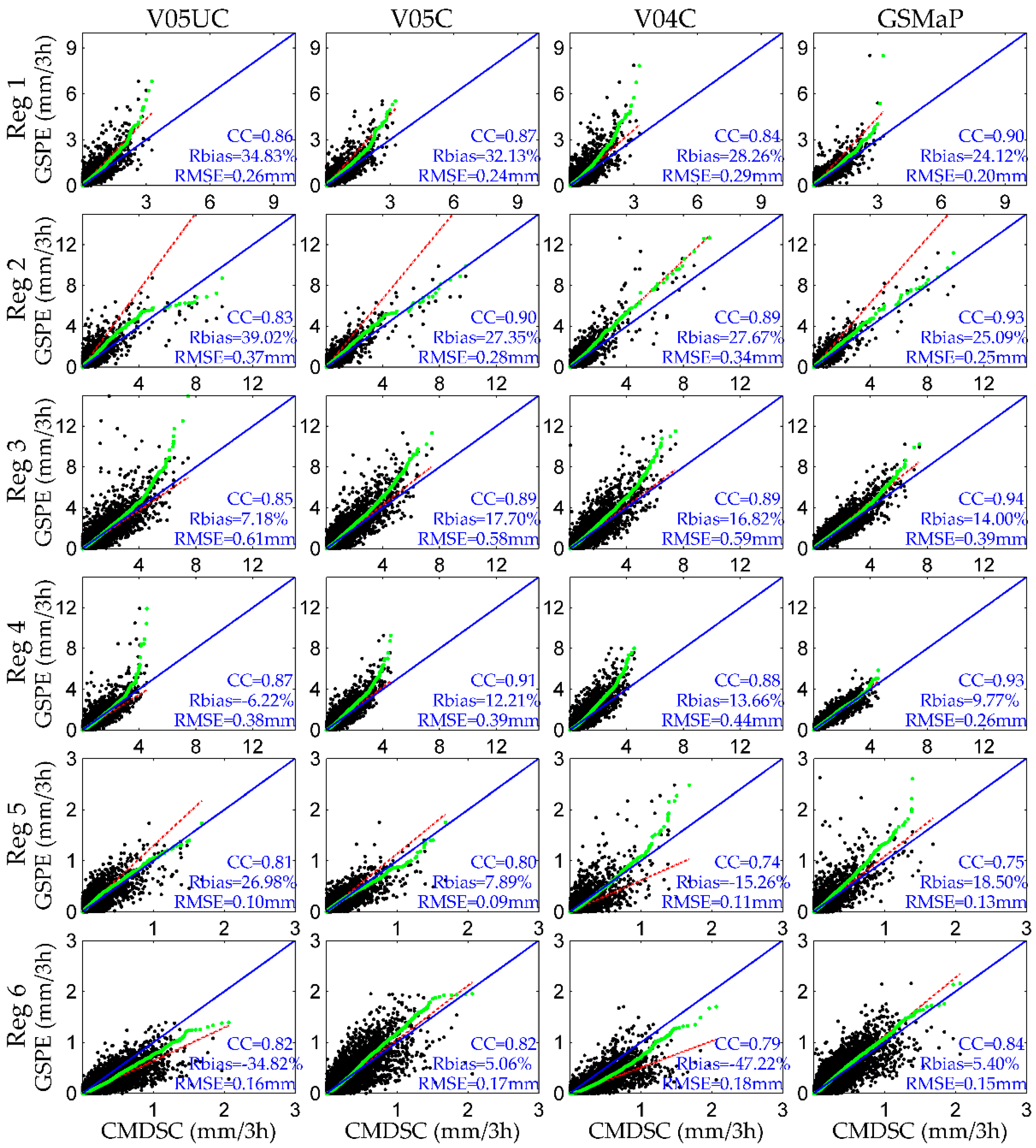
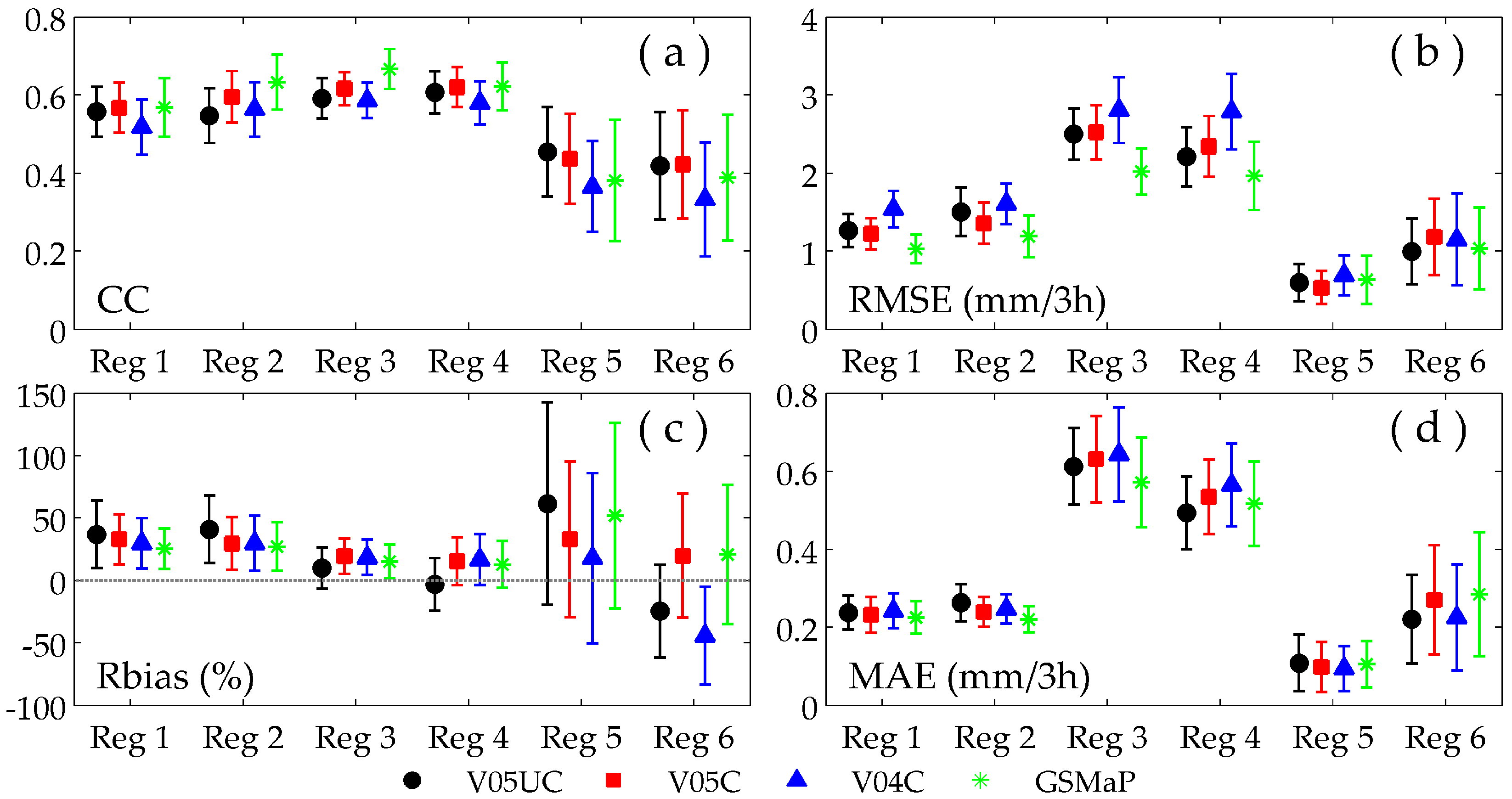
In regional analysis, two calibrated IMERG products (V05C and V04C) showed similar performances in both detecting accurate daily average precipitation and capturing 3-h-scale regional averaged precipitation accumulation over regions 1–4. The uncalibrated V05UC achieved comparable performance to calibrated IMERG products over these regions. This indicated that the latest IMERG (V05UC and V05C) did not achieve superior improvement in these areas, despite the slight improvement in detecting regional heavy precipitation events. Moreover, GSMaP outperformed all of the IMERG products in regions 1–4 in regard to almost all of the metrics. However, all four products should improve their quality in arid areas (Region 5) and the Tibet Plateau (Region 6) for better application.

(3)

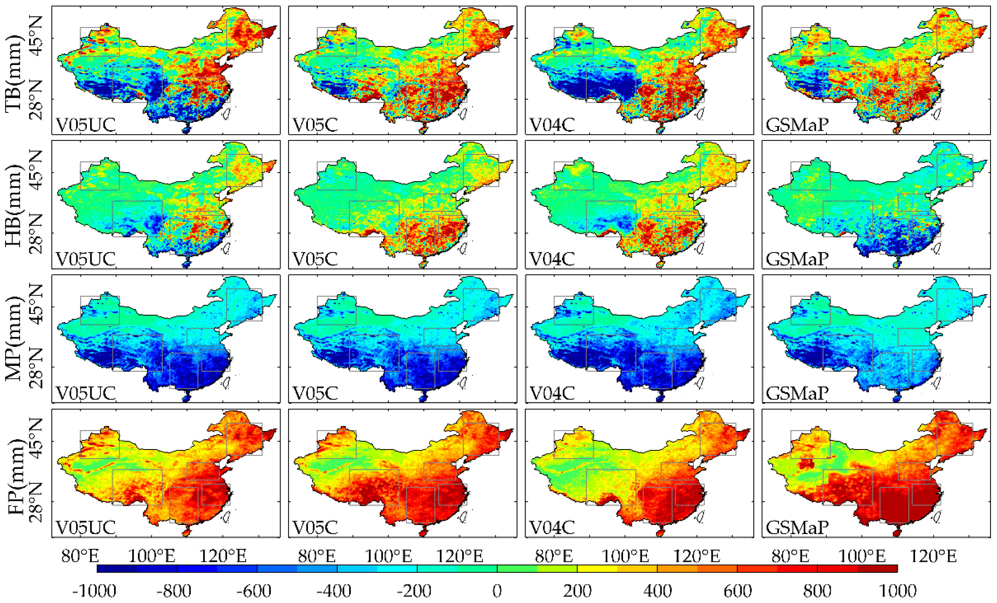
The error components and TB of the four GSPEs showed strong regional differences over mainland China. Much of the overestimations over the North China Plain and northeastern China for IMERG V05 can be traced to significant FP and noticeable HB. Since the GCA used in IMERG V05 was prone to increase the rain rates over the southern Tibetan Plateau and southeastern China, the negative HB had been changed to positive, and FP was significantly enlarged, but could not correct the MP. Thus, the negative TB contained in V05UC had been turned to positive over these regions. V04C had similar error component distributions to V05C except for over the Tibetan Plateau, where larger MP and non-negligible negative HB had generated remarkable TB. For GSMaP, much of the overestimations over the east and south are the comprehensive impact of HB and FP, although MP may counteract some of this impact.

(4)

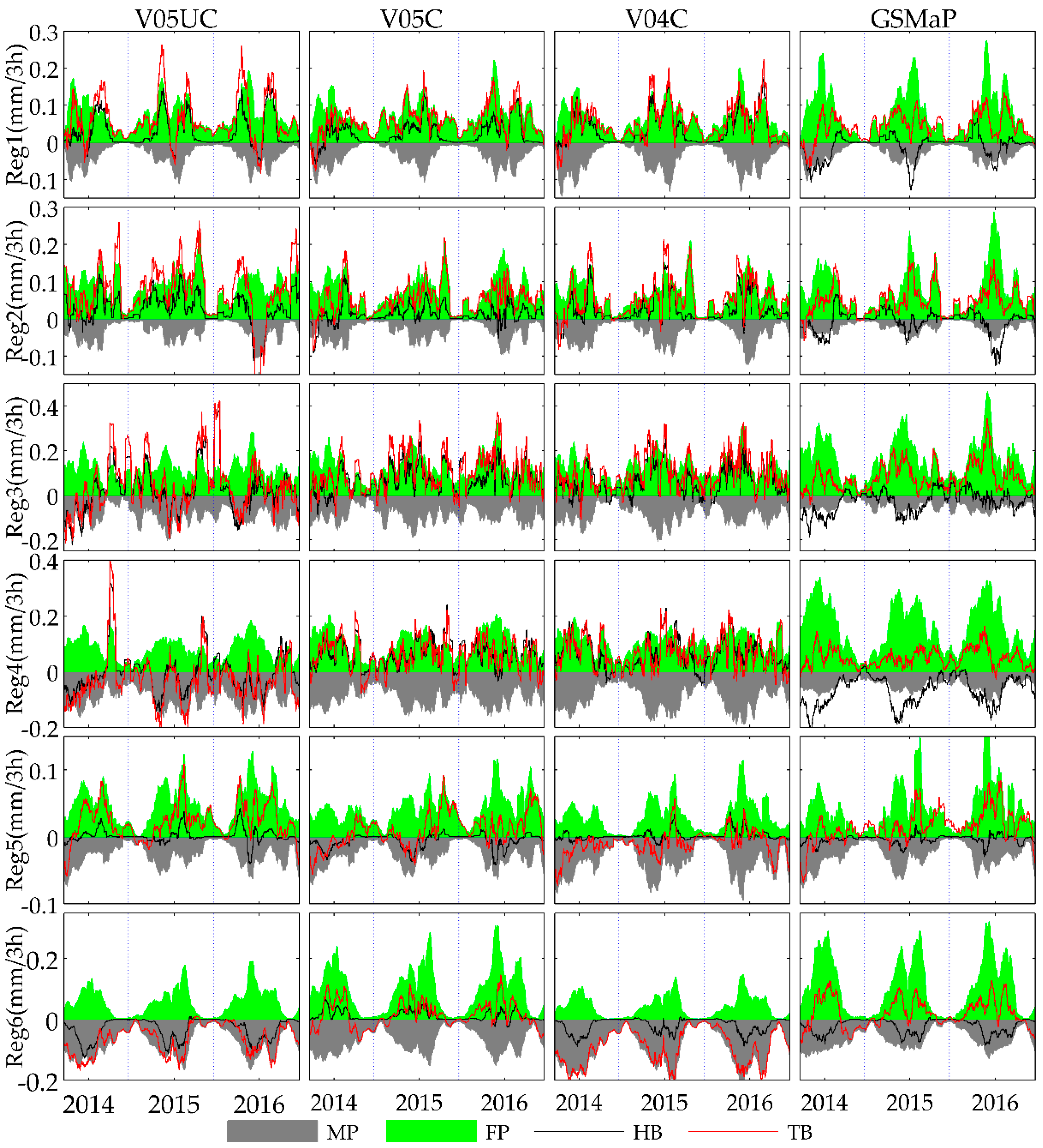
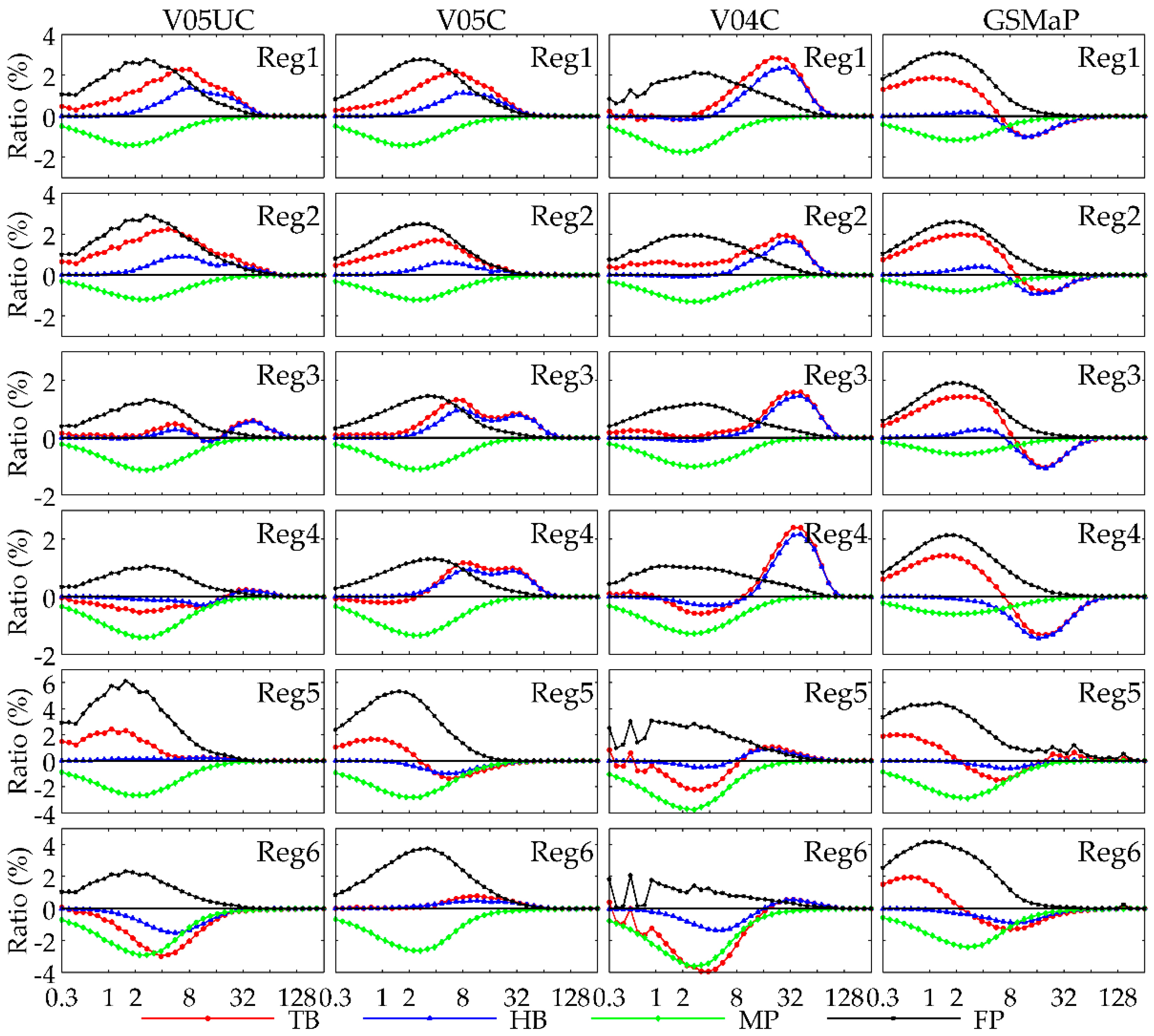
The regional time-series analyses clearly illustrated that the TB resulted from the interaction of the three independent components. The positive HB and FP played a dominant role in the overestimation of IMERG over northeast China (regions 1–2). Benefiting from the mutual melting of FP and MP, the curves of HB in IMERG were very close to the corresponding TB over south China (regions 3–4), although a more obviously positive HB appeared in the calibrated IMERG. The uncertainty in IMERG caused by MP and FP cannot be ignored in high-altitude (Regions 6) and dry (Region 5) areas, particularly for V04C in the Tibetan Plateau, where it showed obvious underestimation principally caused by MP. Larger FP was a main problem of GSMaP over almost the entirety of China. Meanwhile, the HB contained in GSMaP over Region 4 also needs to be noted.

(5)

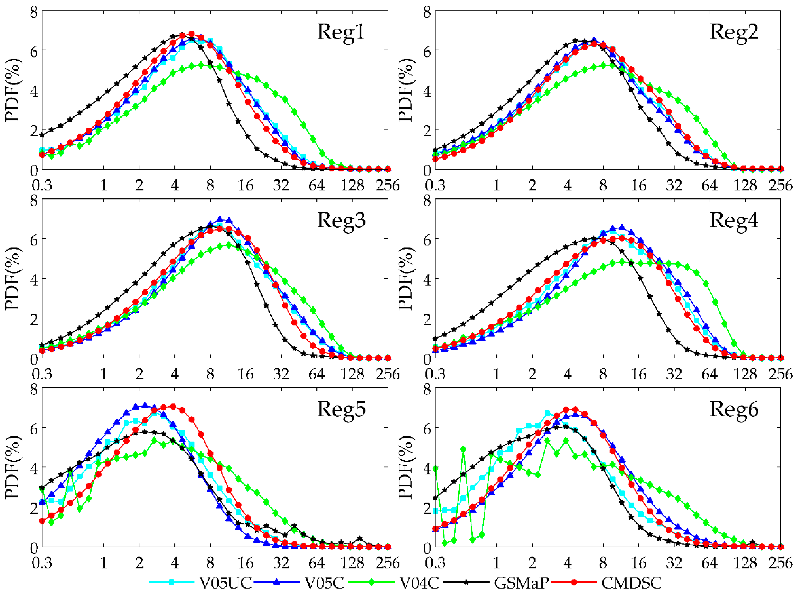
From the perspective of the intensity distribution, V05C can best match the PDF of CMDSC over almost all of the regions, but the overestimation in heavy rain, which was mainly caused by positive HB, was still a large problem. V05UC had better ability than V05C in detecting heavy rain. In addition, GSMaP tended to overrate light rain and underrate heavy rain, particularly for regions 1–4. Such overestimation and underestimation were mainly caused by large FP in light rain and negative HB in heavy rain, respectively.

In summary, the two calibrated V05C and V04C were at about the same level, except for over the Tibetan Plateau, but showed significant improvements from the uncalibrated V05UC over most of the parts of mainland China. Meanwhile, GSMaP was identified to be the best performed precipitation estimation over the east and south of mainland China in spite of the performance reduction over the arid northwest. In order to improve the quality of precipitation, more research methods should be explored, such as the integration of multi-source precipitation information (e.g., satellite-based precipitation estimations, ground gauge/radar observations, reanalysis precipitation products, climate model products, and so on) and the data assimilation method using precipitation related geophysical variables (e.g., soil moisture [59] and snow depth [60]). Besides, further investigations should be also carried out to assess IMERG Level-2 retrieval algorithms and thus provide the underlying insights of how the uncertainty propagates to the IMERG Level-3 precipitation products. Also, more localized studies focused on investigating and improving the quality of GSPEs for specific regions should be encouraged to perfect the calibration algorithms. In addition, as applications are the driving force for technological progress, a broader application of GSPEs in hydrological simulation, disaster forecasting, and water resource management should be called on.

References

1. Hong, Y.; Adler, R.F.; Huffman, G.J.; Pierce, H. Applications of Trmm-Based Multi-Satellite Precipitation Estimation for Global Runoff Prediction: Prototyping a Global Flood Modeling System; Springer: Berlin, Germany, 2010; pp. 245–265. [Google Scholar]
2. Su, J.; Lü, H.; Wang, J.; Sadeghi, A.M.; Zhu, Y. Evaluating the applicability of four latest satellite–gauge combined precipitation estimates for extreme precipitation and streamflow predictions over the upper yellow river basins in China. Remote Sens. 2017, 9, 1176. [Google Scholar] [CrossRef]
3. Hou, A.Y.; Kakar, R.K.; Neeck, S.; Azarbarzin, A.A.; Kummerow, C.D.; Kojima, M.; Oki, R.; Nakamura, K.; Iguchi, T. The global precipitation measurement mission. Bull. Am. Meteorol. Soc. 2014, 95, 701–722. [Google Scholar] [CrossRef]
4. Conti, F.L.; Hsu, K.L.; Noto, L.V.; Sorooshian, S. Evaluation and comparison of satellite precipitation estimates with reference to a local area in the mediterranean sea. Atmos. Res. 2014, 138, 189–204. [Google Scholar] [CrossRef]
5. Dinku, T.; Anagnostou, E.N.; Borga, M. Improving radar-based estimation of rainfall over complex terrain. J. Appl. Meteorol. 2002, 41, 1163–1178. [Google Scholar] [CrossRef]
6. Mei, Y.; Anagnostou, E.N.; Nikolopoulos, E.I.; Borga, M. Error analysis of satellite precipitation products in mountainous basins. J. Hydrometeorol. 2014, 15, 1778–1793. [Google Scholar] [CrossRef]
7. Hong, Y.; Chen, S.; Xue, X.; Hodges, G. Global precipitation estimation and applications. In Multiscale Hydrologic Remote Sensing: Perspectives and Applications; CRC Press: Boca Raton, FL, USA, 2012; pp. 371–386. [Google Scholar]
8. Barrera, D.F.; Ceirano, E.; Zucarelli, G.V. Differences in area-averaged rainfall depth over a mid-size basin from two remote sensing methods of estimating precipitation. In Predictions in Ungauged Basins: PUB Kick-Off, Proceedings of the PUB Kick-Off Meeting Held in Brasilia, 20–22 November 2002; IAHS Publ.: London, UK, 2007. [Google Scholar]
9. Huffman, G.J.; Bolvin, D.; Nelkin, E.; Wolff, D.B.; Adler, R.F.; Gu, G.; Hong, Y.; Bowman, K.P.; Stocker, E.F. The trmm multisatellite precipitation analysis (tmpa): Quasi-global, multiyear, combined-sensor precipitation estimates at fine scales. J. Hydrometeorol. 2007, 8, 38–55. [Google Scholar] [CrossRef]
10. Joyce, R.J.; Janowiak, J.E.; Arkin, P.A.; Xie, P. Cmorph: A method that produces global precipitation estimates from passive microwave and infrared data at high spatial and temporal resolution. J. Hydrometeorol. 2004, 5, 487–503. [Google Scholar] [CrossRef]
11. Sorooshian, S.; Hsu, K.L.; Gao, X.; Gupta, H.V.; Imam, B.; Dan, B. Evaluation of persiann system satellite–based estimates of tropical rainfall. Bull. Am. Meteorol. Soc. 2000, 81, 2035–2046. [Google Scholar] [CrossRef]
12. Kubota, T.; Shige, S.; Hashizume, H.; Aonashi, K.; Takahashi, N.; Seto, S.; Takayabu, Y.N.; Ushio, T.; Nakagawa, K.; Iwanami, K. Global precipitation map using satellite-borne microwave radiometers by the gsmap project: Production and validation. IEEE Trans. Geosci. Remote Sens. 2007, 45, 2259–2275. [Google Scholar] [CrossRef]
13. Ushio, T.; Sasashige, K.; Kubota, T.; Shige, S.; Okamoto, K.I.; Aonashi, K.; Inoue, T.; Takahashi, N.; Iguchi, T.; Kachi, M.; et al. A kalman filter approach to the global satellite mapping of precipitation (gsmap) from combined passive microwave and infrared radiometric data. J. Meteorol. Soc. Jpn. 2009, 87A, 137–151. [Google Scholar] [CrossRef]
14. Mei, Y.; Nikolopoulos, E.I.; Anagnostou, E.N.; Borga, M. Evaluating satellite precipitation error propagation in runoff simulations of mountainous basins. J. Hydrometeorol. 2016, 17, 1407–1423. [Google Scholar] [CrossRef]
15. Chen, F.; Li, X. Evaluation of imerg and trmm 3b43 monthly precipitation products over mainland China. Remote Sens. 2016, 8, 472. [Google Scholar] [CrossRef]
16. Ning, S.; Wang, J.; Jin, J.; Ishidaira, H. Assessment of the latest gpm-era high-resolution satellite precipitation products by comparison with observation gauge data over the Chinese mainland. Water 2016, 8, 481. [Google Scholar] [CrossRef]
17. Tang, G.; Ma, Y.; Long, D.; Zhong, L.; Hong, Y. Evaluation of gpm day-1 imerg and tmpa version-7 legacy products over mainland China at multiple spatiotemporal scales. J. Hydrol. 2016, 533, 152–167. [Google Scholar] [CrossRef]
18. Guo, H.; Chen, S.; Bao, A.; Behrangi, A.; Hong, Y.; Ndayisaba, F.; Hu, J.; Stepanian, P.M. Early assessment of integrated multi-satellite retrievals for global precipitation measurement over China. Atmos. Res. 2016, 176–177, 121–133. [Google Scholar] [CrossRef]
19. Tian, Y.; Peters-Lidard, C.D.; Eylander, J.B.; Joyce, R.J.; Huffman, G.J.; Adler, R.F.; Hsu, K.L.; Turk, F.J.; Garcia, M.; Zeng, J. Component analysis of errors in satellite-basd precipitation estimates. J. Geophys. Res. Atmos. 2009, 114. [Google Scholar] [CrossRef]
20. Xu, S.; Shen, Y.; Du, Z. Tracing the source of the errors in hourly imerg using a decomposition evaluation scheme. Atmosphere 2016, 7, 161. [Google Scholar] [CrossRef]
21. Ning, S.; Song, F.; Udmale, P.; Jin, J.; Thapa, B.R.; Ishidaira, H. Error analysis and evaluation of the latest gsmap and imerg precipitation products over eastern China. Adv. Meteorol. 2017, 2017, 1803492. [Google Scholar] [CrossRef]
22. Yong, B.; Chen, B.; Tian, Y.; Yu, Z.; Hong, Y. Error-component analysis of trmm-based multi-satellite precipitation estimates over mainland China. Remote Sens. 2016, 8, 440. [Google Scholar] [CrossRef]
23. Meng, L.; Long, D.; Quiring, S.M.; Shen, Y. Statistical analysis of the relationship between spring soil moisture and summer precipitation in east China. Int. J. Climatol. 2014, 34, 1511–1523. [Google Scholar] [CrossRef]
24. Yang, Y.; Yi, L. Evaluating the performance of remote sensing precipitation products cmorph, persiann, and tmpa, in the arid region of northwest China. Theor. Appl. Climatol. 2014, 118, 429–445. [Google Scholar] [CrossRef]
25. Guo, Z.H.; Liu, X.M.; Xiao, W.F. Regionalization and integrated assessment of climate resource in China based on gis. Resour. Sci. 2007, 29, 2–9. (In Chinese) [Google Scholar]
26. Shen, Y.; Zhao, P.; Pan, Y.; Yu, J. A high spatiotemporal gauge-satellite merged precipitation analysis over China. J. Geophys. Res. Atmos. 2014, 119, 3063–3075. [Google Scholar] [CrossRef] [Green Version]
27. Xie, P.; Yatagai, A.; Chen, M.; Hayasaka, T.; Fukushima, Y.; Liu, C.; Yang, S. A gauge-based analysis of daily precipitation over East Asia. J. Hydrometeorol. 2007, 8, 607. [Google Scholar] [CrossRef]
28. Shen, Y.; Xiong, A.; Wang, Y.; Xie, P. Performance of high-resolution satellite precipitation products over China. J. Geophys. Res. Atmos. 2010, 115. [Google Scholar] [CrossRef] [Green Version]
29. Shen, Y.; Feng, M.; Zhang, H.; Gao, F. Interpolation methods of China daily precipitation data. J. Appl. Meteorol. Sci. 2010, 21, 279–286. (In Chinese) [Google Scholar]
30. Shen, Y.; Xiong, A. Validation and comparison of a new gauge-based precipitation analysis over mainland China. Int. J. Climatol. 2016, 36, 252–265. [Google Scholar] [CrossRef]
31. Tang, G.; Zeng, Z.; Ma, M.; Liu, R.; Wen, Y.; Hong, Y. Can near-real-time satellite precipitation products capture rainstorms and guide flood warning for the 2016 summer in south China? IEEE Geosci. Remote Sens. Lett. 2017. [Google Scholar] [CrossRef]
32. Shen, Y.; Xiong, A.; Hong, Y.; Yu, J.; Pan, Y.; Chen, Z.; Saharia, M. Uncertainty analysis of five satellite-based precipitation products and evaluation of three optimally merged multi-algorithm products over the tibetan plateau. Int. J. Remote Sens. 2014, 35, 6843–6858. [Google Scholar] [CrossRef]
33. Karaseva, M.O.; Prakash, S.; Gairola, R.M. Validation of high-resolution trmm-3b43 precipitation product using rain gauge measurements over kyrgyzstan. Theor. Appl. Climatol. 2012, 108, 147–157. [Google Scholar] [CrossRef]
34. Huffman, G.J.; Bolvin, D.T.; Braithwaite, D.; Hsu, K.; Joyce, R.; Kidd, C.; Nelkin, E.J.; Sorooshian, S.; Tan, J.; Xie, P. Algorithm Theoretical Basis Document (ATBD) Version 5.1. Available online: https://pmm.nasa.gov/sites/default/files/document_files/IMERG_ATBD_V5.1b.pdf (accessed on 22 January 2018).
35. Huffman, G.J.; Bolvin, D.T.; Nelkin, E.J. Integrated Multi-satellitE Retrievals for GPM (IMERG) Technical Documentation. Available online: https://pmm.nasa.gov/sites/default/files/document_files/IMERG_doc_171117b.pdf (accessed on 22 January 2018).
36. Huffman, G.J.; Bolvin, D.T.; Nelkin, E.J.; Stocker, E.F.; Tan, J. V05 Imerg Final Run Release Notes; NASA/GSFC: Greenbelt, MD, USA, 2017.
37. Omranian, E.; Sharif, H.O. Evaluation of the global precipitation measurement (GPM) satellite rainfall products over the lower Colorado River Basin, Texas. JAWRA J. Am. Water Resour. Assoc. 2018. [Google Scholar] [CrossRef]
38. Okamoto, K.I.; Ushio, T.; Iguchi, T.; Takahashi, N.; Iwanami, K. The global satellite mapping of precipitation (gsmap) project. In Proceedings of the 2005 IEEE International Geoscience and Remote Sensing Symposium, Seoul, Korea, 29 July 2005; pp. 3414–3416. [Google Scholar]
39. Maggioni, V.; Meyers, P.C.; Robinson, M.D. A review of merged high-resolution satellite precipitation product accuracy during the tropical rainfall measuring mission (TRMM) era. J. Hydrometeorol. 2016, 17. [Google Scholar] [CrossRef]
40. Aonashi, K.; Liu, G.; Awaka, J.; Hirose, M.; Kozu, T.; Kubota, T.; Shige, S.; Kida, S.; Seto, S.; Takahashi, N. Gsmap passive microwave precipitation retrieval algorithm: Algorithm description and validation. J. Meteorol. Soc. Jpn. 2009, 87A, 119–136. [Google Scholar] [CrossRef]
41. Ushio, T.; Kachi, M. Kalman Filtering Applications for Global Satellite Mapping of Precipitation (GSMAP); Springer: Dordrecht, The Netherlands, 2010; pp. 105–123. [Google Scholar]
42. Tian, Y.; Peterslidard, C.D.; Choudhury, B.J.; Garcia, M. Multitemporal analysis of trmm-based satellite precipitation products for land data assimilation applications. J. Hydrometeorol. 2007, 8, 1165–1183. [Google Scholar] [CrossRef]
43. Wang, W.; Chen, X.; Shi, P.; Phajmvan, G. Detecting changes in extreme precipitation and extreme streamflow in the dongjiang river basin in southern China. Hydrol. Earth Syst. Sci. 2008, 12, 207–221. [Google Scholar] [CrossRef]
44. Dinku, T.; Ceccato, P.; Grover-Kopec, E.; Lemma, M.; Connor, S.J.; Ropelewski, C.F. Validation of satellite rainfall products over East Africa’s complex topography. Int. J. Remote Sens. 2007, 28, 1503–1526. [Google Scholar] [CrossRef]
45. Li, Z.; Yang, D.; Hong, Y. Multi-scale evaluation of high-resolution multi-sensor blended global precipitation products over the Yangtze River. J. Hydrol. 2013, 500, 157–169. [Google Scholar] [CrossRef]
46. Omranian, E.; Sharif, H.O.; Tavakoly, A.A. How well can global precipitation measurement (GPM) capture hurricanes? Case study: Hurricane harvey. Remote Sens. 2018, 10, 1150. [Google Scholar] [CrossRef]
47. Yong, B.; Chen, B.; Gourley, J.J.; Ren, L.; Hong, Y.; Chen, X.; Wang, W.; Chen, S.; Gong, L. Intercomparison of the version-6 and version-7 TMPA precipitation products over high and low latitudes basins with independent gauge networks: Is the newer version better in both real-time and post-real-time analysis for water resources and hydrologic extr. J. Hydrol. 2014, 508, 77–87. [Google Scholar] [CrossRef]
48. Yuan, F.; Zhang, L.; Win, K.; Ren, L.; Zhao, C.; Zhu, Y.; Jiang, S.; Liu, Y. Assessment of GPM and TRMM multi-satellite precipitation products in streamflow simulations in a data-sparse mountainous watershed in myanmar. Remote Sens. 2017, 9, 302. [Google Scholar] [CrossRef]
49. Beck, H.E.; Vergopolan, N.; Pan, M.; Levizzani, V.; Dijk, A.I.J.M.V.; Weedon, G.P.; Brocca, L.; Pappenberger, F.; Huffman, G.J.; Wood, E.F. Global-scale evaluation of 23 precipitation datasets using gauge observations and hydrological modeling. Hydrol. Earth Syst. Sci. Discuss. 2017, 21, 6201–6217. [Google Scholar] [CrossRef]
50. Michaelides, S.; Levizzani, V.; Anagnostou, E.; Bauer, P.; Kasparis, T.; Lane, J.E.; Michaelides, S. Precipitation: Measurement, remote sensing, climatology and modeling. Atmos. Res. 2009, 94, 512–533. [Google Scholar] [CrossRef]
51. Sun, R.; Yuan, H.; Liu, X.; Jiang, X. Evaluation of the latest satellite–gauge precipitation products and their hydrologic applications over the huaihe river basin. J. Hydrol. 2016, 536, 302–319. [Google Scholar] [CrossRef]
52. Mega, T.; Ushio, T.; Kubota, T.; Kachi, M.; Aonashi, K.; Shige, S. Gauge adjusted global satellite mapping of precipitation (gsmap_gauge). In Proceedings of the General Assembly and Scientific Symposium, Florence, Italy, 9–14 November 2014; pp. 1–4. [Google Scholar]
53. Yong, B.; Ren, L.; Hong, Y.; Gourley, J.J.; Tian, Y.; Huffman, G.J.; Chen, X.; Wang, W.; Wen, Y. First evaluation of the climatological calibration algorithm in the real-time tmpa precipitation estimates over two basins at high and low latitudes. Water Resour. Res. 2013, 49, 2461–2472. [Google Scholar] [CrossRef]
54. Shen, Y.; Pan, Y.; Yu, J.J.; Zhao, P.; Zhou, Z.J. Quality assessment of hourly merged precipitation product over China. Trans. Atmos. Sci. 2013, 36, 37–46. (In Chinese) [Google Scholar]
55. Su, X.; Shum, C.K.; Luo, Z. Evaluating imerg v04 final run for monitoring three heavy rain events over mainland China in 2016. IEEE Geosci. Remote Sens. Lett. 2018, 15, 444–448. [Google Scholar] [CrossRef]
56. Wang, Z.; Zhong, R.; Lai, C.; Chen, J. Evaluation of the gpm imerg satellite-based precipitation products and the hydrological utility. Atmos. Res. 2017, 196, 151–163. [Google Scholar] [CrossRef]
57. Zhao, H.; Yang, S.; You, S.; Huang, Y.; Wang, Q.; Zhou, Q. Comprehensive evaluation of two successive v3 and v4 imerg final run precipitation products over mainland China. Remote Sens. 2017, 10, 34. [Google Scholar] [CrossRef]
58. Wei, G.; Lü, H.; Crow, W.T.; Zhu, Y.; Wang, J.; Su, J. Evaluation of satellite-based precipitation products from imerg v04a and v03d, cmorph and tmpa with gauged rainfall in three climatologic zones in China. Remote Sens. 2017, 10, 30. [Google Scholar] [CrossRef]
59. Crow, W.T.; Berg, M.J.V.D.; Huffman, G.J.; Pellarin, T. Correcting rainfall using satellite-based surface soil moisture retrievals: The soil moisture analysis rainfall tool (smart). Water Resour. Res. 2011, 47, 2924–2930. [Google Scholar] [CrossRef]
60. Lü, H.; Crow, W.T.; Zhu, Y.; Ouyang, F.; Su, J. Improving streamflow prediction using remotely-sensed soil moisture and snow depth. Remote Sens. 2016, 8, 503. [Google Scholar] [CrossRef]
Figure 1. (a) Digital elevation map (DEM) of China; (b) spatial distributions of the four climate districts and locations of the six selected subregions.
Remotesensing 10 01420 g001
Figure 2. Spatial distribution of daily average precipitation (mm/day) during April 2014 and December 2016 at 0.1° × 0.1° resolution derived over mainland China: (a) China Meteorological Date Service Center (CMDSC), (b) V05UC, (c) V05C, (d) V04C and (e) GSMaP.
Remotesensing 10 01420 g002
Figure 3. Scatter plots of daily average precipitation (mm/day) for four GSPEs against CMDSC over six selected regions of mainland China during April 2014 and December 2016.
Remotesensing 10 01420 g003
Figure 4. Quantile–Quantile (Q–Q) plots (green) and scatterplots (black) of 3-h scale regional averaged precipitation accumulation (mm/3 h) from GSPEs against the CMDSC over six regions during April 2014 and December 2016.
Remotesensing 10 01420 g004
Figure 5. Spatial distributions of continuous statistical indices for the chosen four GSPEs at a 3-h time-scale and 0.1° × 0.1° resolution over mainland China: the rows from first to last represent CC RMSE (mm/3 h), Rbias (%), and MAE (mm/3 h), respectively.
Remotesensing 10 01420 g005
Figure 6. Vertical error bars (±σ) of continuous statistical indices for the four chosen GSPEs at a 3-h time-scale over the six selected regions: (a) CC, (b) RMSE (mm/3 h), (c) Rbias (%) and (d) MAE (mm/3 h).
Remotesensing 10 01420 g006
Figure 7. The accumulated error components (mm) of the four GSPEs (i.e., V05UC, U05C, V04C, and GSMaP) for the entire study period from April 2014 to December 2016 at a 3-h and 0.1° × 0.1° resolution.
Remotesensing 10 01420 g007
Figure 8. Spatial distributions of categorical statistical indices—false alarm ratio (FAR), probability of detection (POD), and critical success index (CSI)—of the four GSPEs—i.e., uncalibrated Integrated Multi-satellitE Retrievals for the GPM (IMERG) V05 (V05UC), gauge-calibrated IMERG V05 (VU05C), gauge-calibrated IMERG V04 (V04C), and Global Satellite Mapping of Precipitation (GSMaP)—for the entire study period from April 2014 to December 2016 at a 3-h and 0.1° × 0.1° resolution over mainland China.
Remotesensing 10 01420 g008
Figure 9. Regionally averaged time series of error components and total bias for four GSPEs (i.e., V05UC, U05C, V04C, and GSMaP) at a 3-h resolution.
Remotesensing 10 01420 g009
Figure 10. Probability density function of 3 h of precipitation intensity for four GSPEs (i.e., V05UC, U05C, V04C, and GSMaP) and the gauged observation in six selected regions.
Remotesensing 10 01420 g010
Figure 11. Probability density function of total bias, hit bias, missed precipitation, and false precipitation intensity for four GSPEs (i.e., V05UC, U05C, V04C, and GSMaP) from April 2014 to December 2016 in six selected regions.
Remotesensing 10 01420 g011