Source Model and Stress Disturbance of the 2017 Jiuzhaigou Mw 6.5 Earthquake Constrained by InSAR and GPS Measurements

Abstract

Seismogenic fault geometry, especially for a blind fault, is usually difficult to derive, based only on the distribution of aftershocks and interference fringes of Interferometric Synthetic Aperture Radar (InSAR). To better constrain the fault geometry of the 2017 Jiuzhaigou Mw 6.5 earthquake, we first carried out a nonlinear inversion for a single fault source using multi-peak particle swarm optimization (MPSO), Monte Carlo (MC), and Markov Chain Monte Carlo (MCMC) algorithms, respectively, with constraints of InSAR data in multiple SAR viewing geometries. The fault geometry models retrieved with different methods were highly consistent and mutually verifiable, showing that a blind faulting with a strike of ~154° and a dip angle of ~77° was responsible for the Jiuzhaigou earthquake. Based on the optimal fault geometry model, the fault slip distribution jointly inverted from the InSAR and Global Positioning System (GPS) data by the steepest descent method (SDM) and the MC method showed that the slip was mainly concentrated at the depth of 1–15 km, and only one slip center appeared at the depth of 5–9 km with a maximum slip of about 1.06 m, some different from previous studies. Taking the shear modulus of μ = 32 GPa, the seismic moment derived from the distributed slip model was about 7.85 × 10¹⁸ Nm, equivalent to Mw 6.54, which was slightly larger than that from the focal mechanism solutions. The fault spatial geometry and slip distribution could be further validated with the spatial patterns of the immediate aftershocks. Most of the off-fault aftershocks with the magnitude > M2 within one year after the mainshock occurred in the stress positive stress change area, which coincided with the stress triggering theory. The static Coulomb stress, triggered by the mainshock, significantly increased at the Tazang fault (northwest to the epicenter), and at the hidden North Huya fault, and partial segments of the Minjiang fault (west of the epicenter).

1. Introduction

On the 8 August 2017, an M_W 6.5 earthquake struck Jiuzhaigou (103.82°E, 33.20°N) in Sichuan Province, China, with a focal depth of approximately 20 km (http://www.csi.ac.cn). The epicenter was located just at the intersection of the Tazang fault, Minjiang fault and Huya fault (Figure 1). Several strong earthquakes, with magnitudes larger than M_W 6.0, have occurred in this region including the 1933 M_W 7.5 Diexi earthquake along the southern segment of the Minjiang fault [1] and the 1976 Songpan earthquake swarm of M_W 7.2, M_W 6.5, and M_W 7.2 [2], along the Huya fault. The Huya and Minjiang faults control the eastern and western boundary of the Minshan uplift zone, respectively. The NS-trending Minjiang fault extends northward to the Tazang fault and southward to the Wenchuan–Maowen fault. The NNW-trending Huya fault extends southward to the Pingwu-Qingchuan fault and northward to the Snow Mountain fault. However, the segment of the Huya fault, north of the Snow Mountain, is a blind segment [3]. The Jiuzhaigou earthquake recently occurred in this blind segment of the Huya fault [4], which provided an opportunity and a challenge to identify the blind fault geometry through the geodetic data.

Results from the field investigation reported immediately after the event showed that no significant surface rupture was found around the epicenter [4]. There were significant discrepancies among the focal mechanism solutions by several organizations, e.g., the Global Centroid Moment Tensor (GCMT), United States Geological Survey (USGS), and China Seismic Information (CSI), in terms of the fault geometric parameters, while these solutions showed that the rupture was dominated by strike-slip. The near-field full seismic waveform inversion for the focal mechanism indicated that the Jiuzhaigou earthquake was mostly dominated by a left-lateral strike-slip [5], with a strike direction of 153°. The coseismic slip distribution constrained by the Sentinel-1A/B ascending and descending interferograms showed that the earthquake was produced by a left-lateral strike-slip, on a southwest-dipping fault plane [6], with a strike direction of 153°, or on two northeast-dipping fault planes [7] with the strikes of 329° and 341°, respectively. Horizontal displacements in the near field as indicated by GPS data suggested the presence of a fault dipping to the northeast [8] with a strike direction of 326°. Constrained by the InSAR and GPS data, optimal dip angles of 80° and 81° for the Jiuzhaigou earthquake with the strike direction of 155° were reported [9,10], respectively. The results of three faulting segments, used to fit seismic waveforms and InSAR data, indicated that the Jiuzhaigou earthquake occurred on a young fault system [11].

There are significant inconsistencies in the aforementioned studies regarding the fault geometric parameters. These are mainly due to the fact that most of the parameters of fault geometry models are directly constructed using aftershocks and interference fringes [6,7,8,9,10,11,12]. Discrepancies in the fault geometry may inevitably result in the inconsistency of fault slip models, and even the deviation of static Coulomb stress changes at the nearby faults. Therefore, further study is still needed to optimize the source models as more InSAR and GPS data becomes available. In addition, the static Coulomb stress distribution due to the mainshock is also necessary to quantify for seismic hazard assessment.

In this study, we first utilized the SAR data of Sentinel-1A/B and RADARSAT-2 (

Table 1. The InSAR data of the Jiuzhaigou earthquake.

Satellite	A/D	Image Time		Polarization	ΔT/day	B⊥/m	ΔH2π/m	Abbr.
		Pre-Quake	Post-Quake
Sentinel-1	A	20170730 A	20170811 A	VV	12	−35.79	~433.5	S1A
	D	20170725 A	20170812 B	VV	18	11.96	~1242.3	S1D
Radarsat-2	A	20170530	20170810	HH	72	46.48	~250.5	R2A

A and D represent the ascending orbit and descending orbit, respectively. The superscript A and B represent the Sentinel-1A and Sentinel-1B satellites, respectively. ΔT is the time baseline with a unit of day. B_⊥ is the vertical baseline with a unit in meters. ΔH_2π is the height of ambiguity with a unit in meters. Abbr. is the abbreviation of corresponding interferogram pairs.

) to build up the coseismic deformation fields in multiple SAR viewing geometries. We inverted the coseismic measurements for the geometric parameters of the seismogenic fault with the algorithms of multi-peak particle swarm optimization (MPSO) + Monte Carlo (MC) [13,14], and Markov Chain Monte Carlo (MCMC) [15], respectively. A joint inversion from the InSAR data and GPS measurements was conducted to determine the slip distribution of the earthquake with the steepest descent method (SDM) [16] and MC method. The static Coulomb disturbances were also calculated using the mainshock rupture and the nearby receiving faults separately to reveal the triggering relationship between the Coulomb stress and aftershocks, and to analyze the seismic potentiality of the nearby faults due to the Jiuzhaigou earthquake. Finally, the discrepancies of several existing distribution models and the Coulomb stress disturbances are discussed.

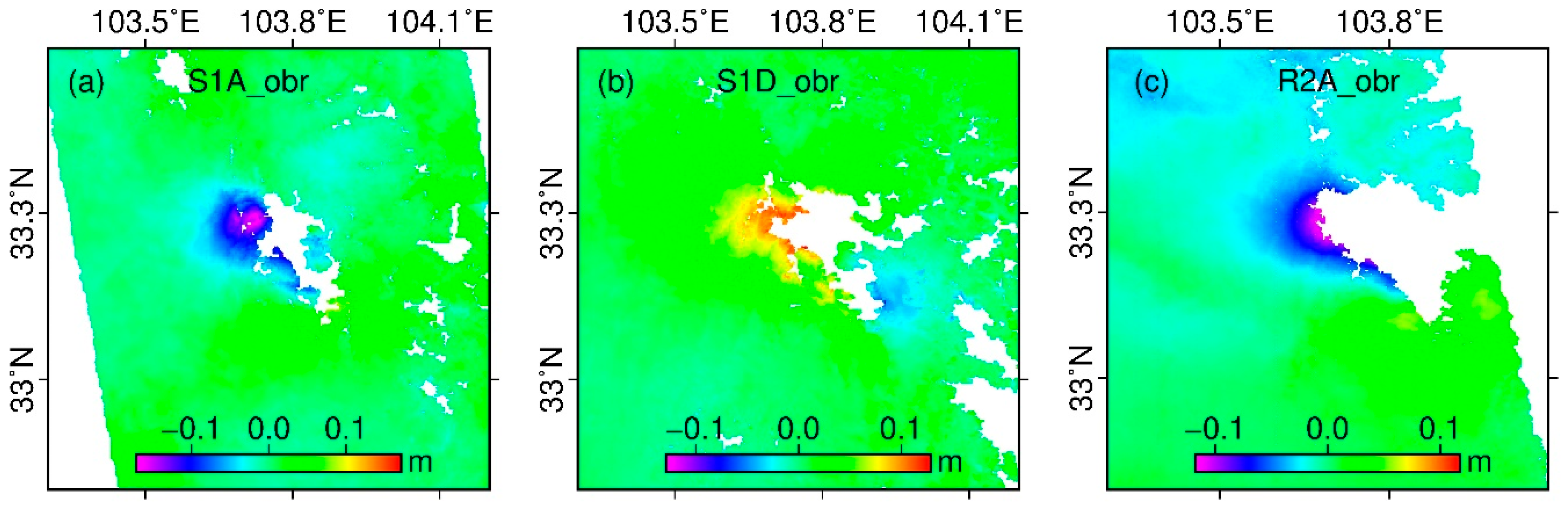
2. InSAR Coseismic Deformation Measurements

The SAR data used in this study included the Single Look Complex (SLC) data in ascending and descending orbits from the Sentinel-1A/B and RADARSAT-2 satellite platforms (Table 1), operating at the C band with a radar wavelength of about 5.6 cm. The coseismic interferometry pairs of the Sentinel-1 ascending, descending, and RADARSAT-2 ascending orbits are referred to the S1A, S1D, and R2A in this study, respectively.

We used the InSAR Scientific Computing Environment (ISCE) [17] software developed by the Jet Propulsion Laboratory (JPL) and Stanford University to generate interferograms of the three image pairs (Table 1). The precise orbit data for S1A and S1D were used to reduce potential orbit errors. A Shuttle Radar Topography Mission (SRTM) digital elevation model with a spatial resolution of about 30 m [18] was used to remove the topographic contribution of the interferograms. The interferograms were then unwrapped with the SNAPHU method [19]. For the Sentinel-1A/1B data, we mosaicked the multiple bursts in the same swath and the three swaths in a track. A strict, high-precision data alignment is required for the Sentinel-1 SAR data. In addition, a spectral method has been proposed to remove the phase jumps due to steep frequency variations along the azimuth [20]. The ISCE can process the Sentinel-1 interferometry efficiently and allows for the extraction of the Region of Interest (ROI) from the entire mosaic image, which can greatly reduce the computation time.

The interferogram pairs have short vertical baselines smaller than 50 m (Table 1), which are beneficial for decreasing the contribution of potential topographic phase errors and maintaining high coherence. The heights of ambiguity of the S1A, S1D, and R2A interferogram pairs for a 1-m error in the terrain can introduce a ~6.5 × 10⁻³ cm, ~2.2 × 10⁻³ cm, and ~1.1 × 10⁻² cm deformation deviation, respectively. The vertical accuracy of SRTM 1 is generally better than ~10 m [21]; therefore, the influence of topography errors is very small and was ignored in this study. In addition, timely satellite observations after the mainshock are beneficial for excluding postseismic deformation contamination. The ionospheric errors were not negligible for the InSAR measurement with a long wavelength of the L or P band; however, they were greatly weakened for the C band with a relatively shorter wavelength [22]. Significant topography correlated atmospheric screens (APS) could be observed in all three interferograms. To reduce the effects of APS, independent APS simulations with a GACOS online system [23,24] were used to correct the interferograms for APS. We found that the tropospheric disturbance of the S1D interferograms was effectively reduced, and the variance of the far field noise in the interferogram decreased from 52 mm² to 41 mm².

The coseismic deformation fields of the InSAR measurements are shown in Figure 2. The coseismic deformation fields can be divided into east and west zones by the nearly NW-trending boundary. The west zone has a larger deformation magnitude and coverage than the east zone. The western deformation fields of S1A and R2A with ascending orbits demonstrated subsidence in the line-of-sight (LOS) direction, opposite to those from the S1D with descending orbit, which indicated that the predominant deformation was a horizontal component as the major difference between the ascending and descending InSAR measurements was due to the contributions of horizontal motions. Therefore, the InSAR results in multiple viewing geometries, particularly in the descending and ascending directions, can better serve the determination of the focal mechanism of the Jiuzhaigou earthquake.

3. Geodetic Modeling

First, we estimated the fault geometry parameters from down-sampling the InSAR data. Then, we jointly inverted the InSAR and GPS data to obtain the fault slip distribution as well as its uncertainties.

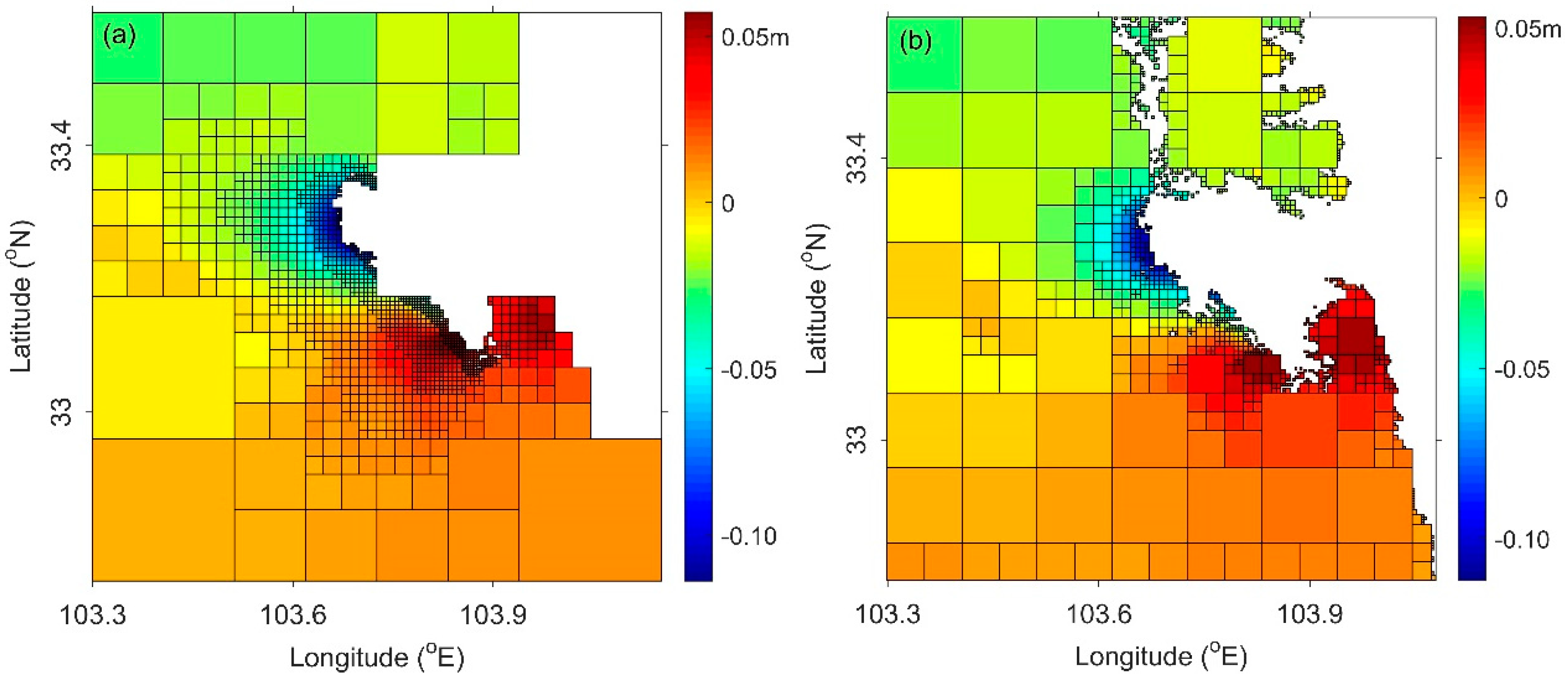
3.1. Data Down-Sampling

The conventional quadtree down-sampling method may produce high densities of data far from the deformation center in the presence of non-deformation noise, decorrelation, or phase-unwrapping errors, which may possibly affect the solution accuracy of fault geometric parameters and slip distributions. Here, we used the Resolution Based method (R_Based) [25] to down-sample the coseismic deformation fields. The R_Based method considers the resolution between the deformation data and fault slip model. It uses a priori fault plane source to determine the data resolution matrix and down-sample the data with spatial variables in which it becomes possible to down-sample the data densely in the near-field of the seismogenic fault and sparsely in the far-field (Figure 3), which can effectively decrease the far-field noise influence in the following inversion. Through R_Based resampling, we obtained 1953, 1581, and 1517 deformation points from the interferograms of the S1A, S1D, and R2A, respectively, with variable incidence angles and azimuth angles to the coordinates of InSAR data.

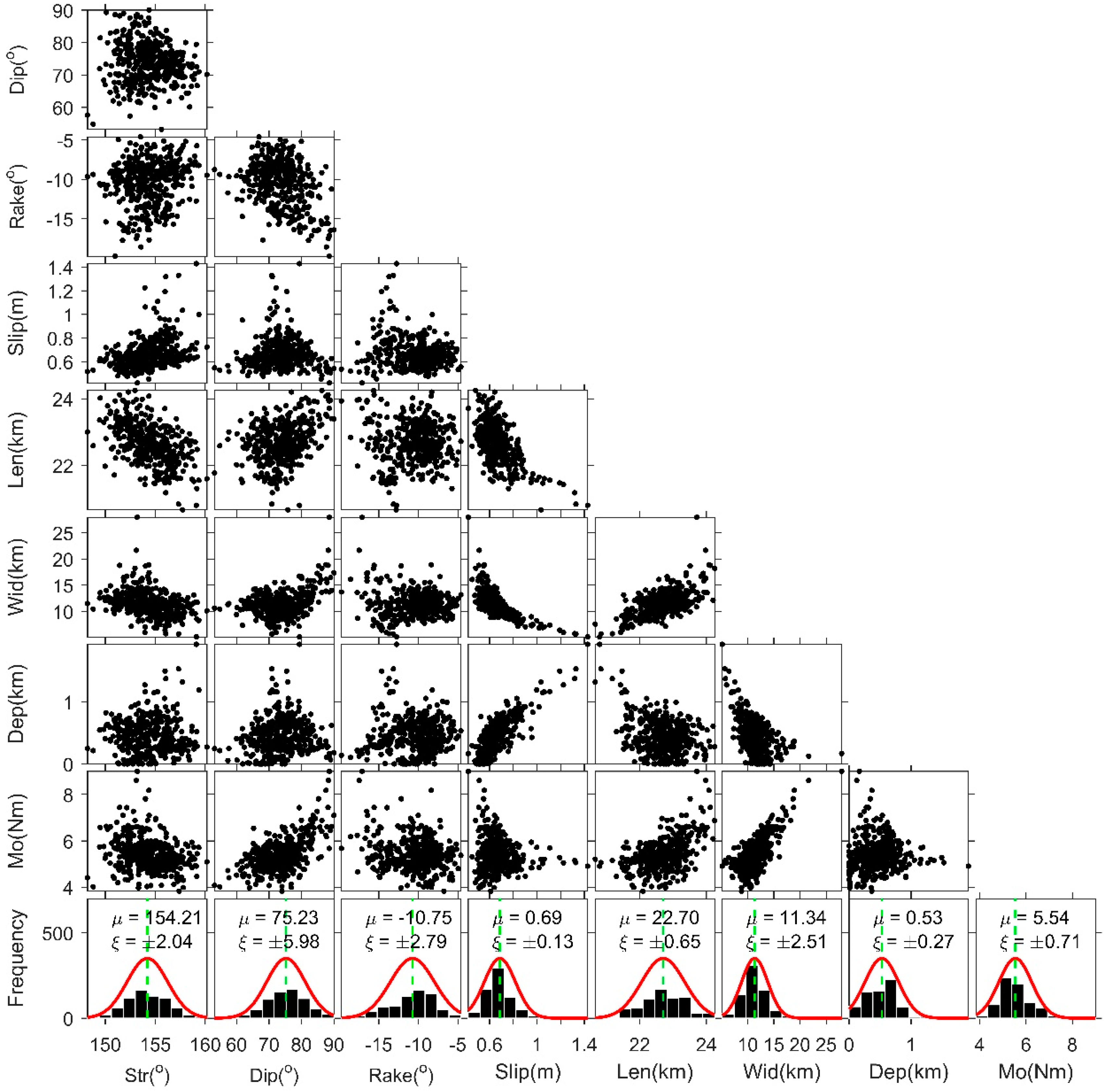
3.2. Nonlinear Inversion for Fault Geometry

According to the focal mechanism of the mainshock and aftershocks of the Jiuzhaigou earthquake [5], the seismic sequence was dominantly controlled by a vertical left-lateral strike-slip fault with a SSE strike direction. The long axis orientation of isoseismic, spatially linear distributions of the aftershocks, and earthquake-triggered bedrock collapses or landslides in the epicenter all indicate that the seismogenic faulting was oriented NNW [4]. The focal mechanism solutions of the GCMT, USGS, and CSI also showed that the SSE-oriented rupture controlled this event. The long axis azimuth of the InSAR deformation fringes coincided with the SSE-oriented rupture. Therefore, we assumed that the seismogenic fault was an NNW-SSE striking and left-lateral strike-slip fault, which has also been adopted by most of the preceding researches [6,8,9,10,12].

To build the fault model more reasonably, we adopted two methods to invert the fault geometry parameters. If the geometry parameters inverted by different methods were similar, we believed that the results were reliable and could be cross-validated. However, if the opposite was true, the results were unreliable.

3.2.1. MPSO+MC Method

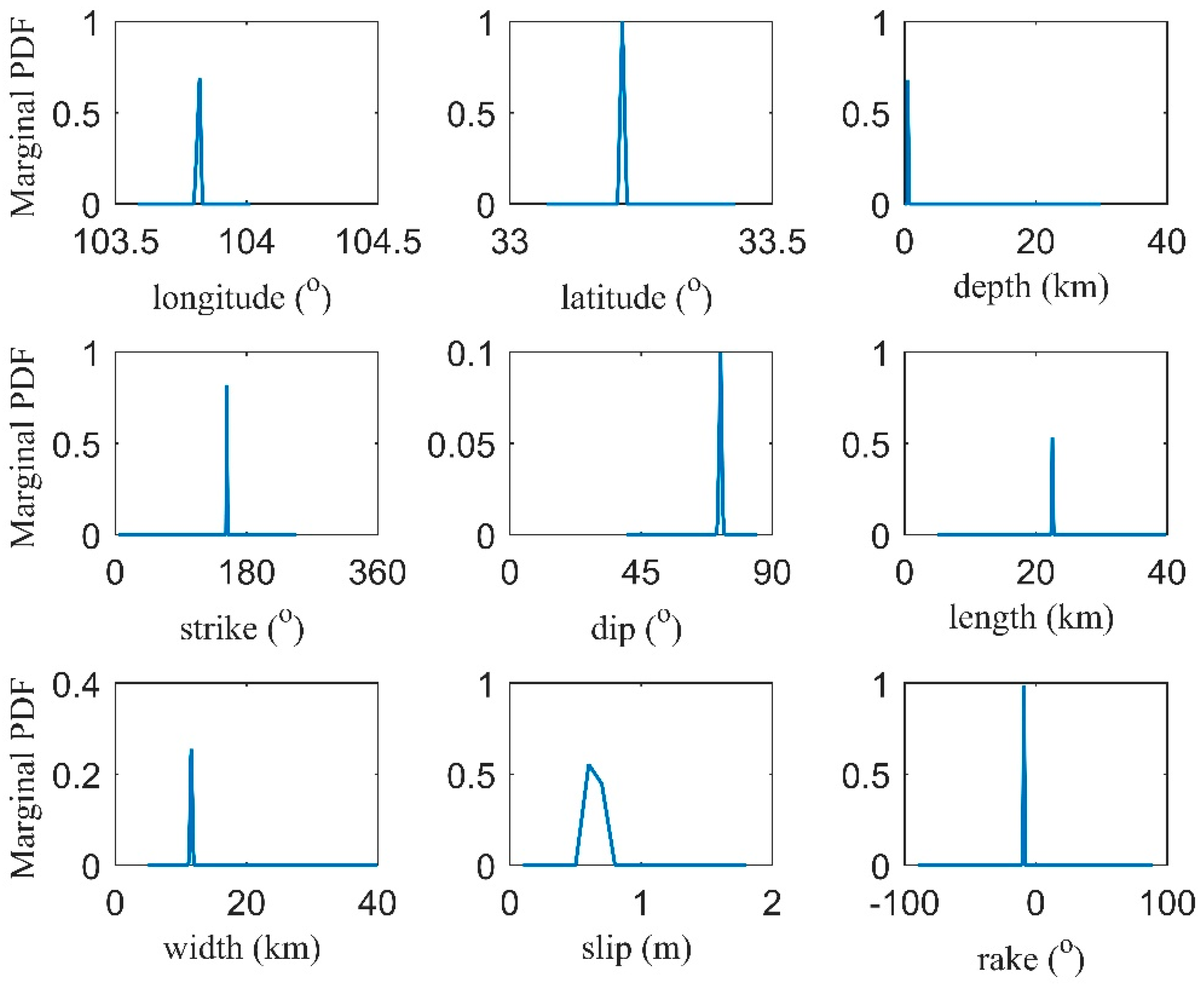
Based on the hypothesis of uniform slip, the MPSO algorithm [13] was used to invert for the geometric parameters of the fault including the fault location, length, width, strike, buried depth, dip angle, slip magnitude, and rake angle. The MPSO nonlinear inversion algorithm has been successfully applied to multiple earthquakes [26,27]. The relative weights of the coseismic deformation fields of S1A, S1D, and R2A were separately determined at 0.17, 0.43, and 0.40 by the far-field noise levels, which were evaluated by the best-fit 1D covariance function [14].

By minimizing the root mean square (RMS) deviation between the measurements and model values, an optimal solution of the geometric parameters of the fault can be obtained. However, the MPSO method alone cannot estimate the inversion errors of the fault parameters. Referring to the MC method [14], we further generated 100 groups of InSAR measurement data with random noise through the full Variance–Covariance Matrix (VCM) in the far field, assuming that the noise was isotropic in the image. With regard to the constraints imposed by the noisy data, we again performed global search 100 times to obtain 100 sets of solutions of fault parameters. Then, the mean and standard deviation of the fault parameters were solved by the Gaussian distribution statistics of the 100 sets of solutions (Figure 4). The standard deviation was considered as the error of the fault geometry parameter.

The geometrical parameters of the seismogenic fault retrieved by the MPSO+MC algorithm are shown in

Table 2. The source mechanism parameters retrieved by different methods.

Source	Top Fault Center			Length/km	Width/km	Strike/(°)	Dip/(°)	Rake/(°)	Slip/m	Depth/km	Mo/×1018 Nm	Mw
	X/(°)	Y/(°)	Z/km
F1	103.831 ± 0.006	32.221 ± 0.005	0.53 ± 0.27	22.70 ± 0.65	11.34 ± 2.51	154.21 ± 2.04	75.23 ± 5.98	−10.75 ± 2.79	0.69 ± 0.13	-	5.54 ± 0.71	6.44 ±0.03
F2	103.816 C ± 0.001	33.211 C ± 0.001	0.534 ± 0.001	22.52 ± 0.01	11.59 ± 0.02	153.36 ± 0.02	72.21 ± 0.21	−9.15 ± 0.02	0.65 ± 0.01	-	5.43 ± 0.10	6.43 ± 0.01
S1	-	-	-	40.0	22.0	154.21	77.0	−7.86 A ± 0.31 −10.37 MS ± 0.34	0.28 A ± 0.01 1.06 M ± 0.02	6.84 MS ± 0.33	7.85 ± 0.13	6.54 ± 0.01
Shan et al. [6]	-	-	-	40	30	153	50	−9 A	~1	~8 MS	-	6.50
Zhang et al. [12]	-	-	-	32	30	153	84	−19.5 A	~1	~12 MS	6.61	6.50
Ji et al. [7]	-	-	-	N:26	26	341	<16 km:90	-	~0.77 M	-	-	6.46
							>16 km:61
	-	-	-	S:20	26	329	<16 km:90	-
							>16 km:75
Wang et al. [8]	-	-	-	80	40	326	60	−15A	0.4 M	-	-	6.40
Zhao et al. [9]				35	25	155	80	−10A	~1.3 M	~6MS	6.75	6.50
Nie et al. [10]				40	30	155	81	−11A	~0.85 M ~0.18 A	~11MS	6.635	6.49
Yang et al. [5]	-	-	-	-	-	150	80	−20	-	~22	-	6.36
						244	70	−169
USGS	-	-	-	-	-	246	57	−173	-	13.5	7.228	6.5
						153	84	−33
GCMT	-	-	-	-	-	242	77	−168	-	14.9	7.62	6.5
	-	-	-	-	-	150	78	−13
CSI	-	-	-	-	-	326	62	−15	-	11.0	-	6.5
	-	-	-	-	-	64	77	−151

The F1 and F2 are separately the uniform slip fault model retrieved by the MPSO+MC and the MCMC method; the S1 are the distributed slip models derived by the SDM+MC method based on the extension of F1 with an optimize dip angle. Models from References [6,7] are with the inversion of the InSAR data; the model of Reference [5] is with the inversion of seismic waves; the model in Reference [8] is with the inversion of the GPS data; the model from Reference [12] is derived from the joint inversion of the InSAR and seismic wave data; the models in References [9,10] are with the joint inversion of the InSAR and GPS data. The superscript C represents the center point of the fault plane, the superscript A represents the average value, the superscript M represents the maximum, and the superscript MS represents the maximal slip.

, and represented by F1. According to the MPSO+MC inversion, the strike, dip angle and rake angle of the fault were closer to the GCMT and USGS solutions than the CSI solutions. Assuming the shear modulus was μ = 32 GPa, the seismic moment of the Jiuzhaigou earthquake derived by the MPSO+MC algorithm was about (5.54 ± 0.71) × 10¹⁸ Nm, equivalent to a moment magnitude of Mw 6.44 ± 0.03, slightly smaller than those of the focal mechanism solutions.

3.2.2. MCMC Method

One problem of the Akaike’s Bayesian Information Criterion (ABIC) inversion algorithm [28] is that the model space integration cannot be correctly resolved under non-negative constraints. Therefore, one full Bayesian inversion method has been proposed, which adopts the more reasonable sampling method of the Markov Chain Monte Carlo [29]. However, if the priori constraints are too strong, the solution of the MCMC method will be not unique, which may cause the multimodal posterior distribution to possibly fall into a local minimum solution. The maximum value of complex functions with multiple peaks can be found by the simulated annealing (SA) algorithm, which can effectively avoid falling into the local minimum solution [15]. Furthermore, the MCMC method improved by the SA algorithm can make the acceptance probability cool and converge faster.

Although the above MCMC method was suitable for the optimization problem with non-negative constraints, we adopted the method to invert the geometric parameters of the fault with the boundary constraints of variables. The Markov chain can be divided into the burn-in and resampling stage. A relatively long Markov chain is needed to ensure the solution convergence. The total length of the Markov chain was composed of 1 × 10⁶ seeds, the length of the burning and resampling stage were separately composed of 0.5 × 10⁶ seeds, and the resampling interval was set as 100 seeds. The advantage of the MCMC algorithm is that not only can the mean value of geometric parameters be retrieved, but also the error range and marginal probability density function (MPDF) of each parameter can be estimated. After resampling the second stage of the Markov chain, the mean model can be obtained by averaging the sampling space. The results showed that the MPDF of the fault parameters were consistent with the normal Gauss distribution (Figure 5).

The geometrical parameters of the seismogenic fault retrieved by the MCMC algorithm are shown in Table 2, and represented by F2. Taking the shear modulus as μ = 32 GPa, the seismic moment of the Jiuzhaigou earthquake was about (5.43 ± 0.10) × 10¹⁸ Nm, equivalent to the moment magnitude Mw 6.43 ± 0.01, which was very close to the MPSO+MC algorithm.

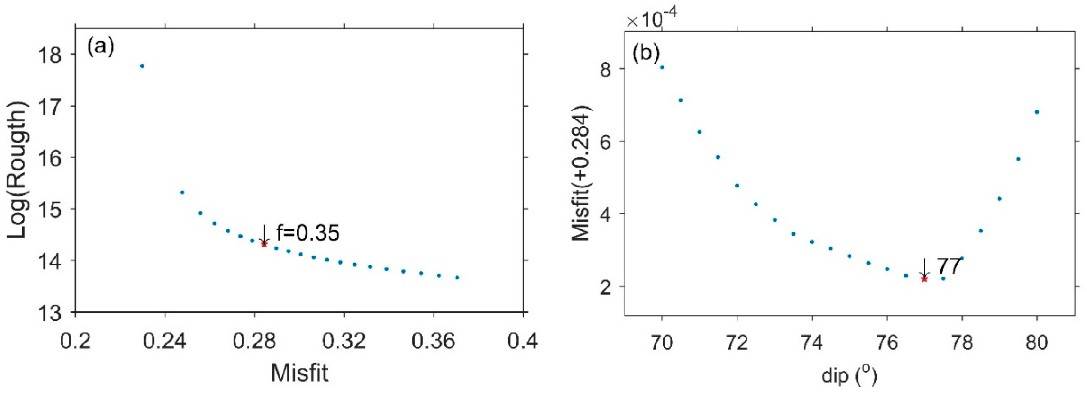
3.3. Inversion for Fault Slip Distribution

Except for about a 3° deviation in the dip angle of the F1 and F2 models, the other parameters were highly consistent with each other. Due to the high similarity of the fault geometry parameters determined by the different nonlinear inversion methods, we believed that the fault geometry models were reliable. As there was only a slight difference between the F1 and F2 models, the F1 model was considered for inversion for the fault slip distribution. Besides the InSAR data, we also adopted the coseismic displacements of 10 GPS stations [8] to constrain the slip distribution.

The fault model of F1 extended along the strike and dip directions to a length of 40 km and 22 km, respectively. In order to discretize the fault plane into a reasonable patch size, we first performed checkerboard tests. Synthetic slip distributions with patch sizes of 2 km, 4 km and 6 km were used as input models to calculate LOS displacements at the multiple view geometries of the InSAR and GPS locations, and then the synthetic displacements were subsequently used to invert for the distributed slip basing on the same regularization that was applied in the forward-model. The checkerboard tests showed that the slips down to a depth of 18 km were well recovered, with a patch size of 6 km (Figure S1). According to previous studies [30,31], a uniform fault patch size may be experimentally about 20% of the recoverable spatial resolution of the checkerboard at the depth, above which most of slip occurs. Therefore, the extended fault plane was divided into 880 patches, each with a size of 1 km × 1 km in this study.

Based on the result from the field investigation [4], we assumed there was no sliding at the top boundary of the fault plane. The Crust1.0 model [32] and EDGRN software, a layered half-space model [33] were employed to compute Green’s functions. Considering that the accuracy of GPS is better than that of InSAR, we set its initial relative weight to 1 and set the relative weight ratio of InSAR to (0, 1) with the same value used in the nonlinear inversion of fault geometry. Then, by using the mean RMS residuals ratio of GPS and the InSAR measurement in the initial inversion of the slip distribution, an optimal factor of 10:1 was chosen as the relative weight ratio of the GPS and InSAR data after multiple calculations.

The reasonable smoothing factor was set to 0.35, which was determined by the trade-off curve of the relative fitting residuals of the Misfit and Roughness (Figure 6a). In order to further optimize the dip angle, the slip distributions with a variable dip angle from 70° to 80° with an interval of 0.5° were inverted, separately; and the optimized dip angle was determined to be 77° by the trade-off curve between the Misfit and dip angle (Figure 6b).

The uncertainty of the slip distributions could not be directly obtained by the single SDM inversion. Therefore, we integrated the MC method with the SDM method. First, the SDM inversion was performed 100 times, each time with the input data generated by observational LOS displacement plus random noise using the VCM method in the far field. Then the 100 sets of slip distribution solutions were analyzed statistically to calculate the average and standard deviation of the slip distributions (Figure 7 and Table 2).

Using the distributing slip model of S1 to forward calculate the deformation fields and to compare with the InSAR and GPS data, the residuals obtained are shown in Figure 8. The mean residuals of the retrieved S1A, S1D, and R2A interferogram pairs were about 1.9 cm, 1.4 cm, and 0.8 cm, respectively. The mean residual of the GPS horizonal deformation was about 2.0 mm. Overall, the residuals were not systematic spatially, indicating that the fault slip distributions model was a good match for the geodetic measurement data.

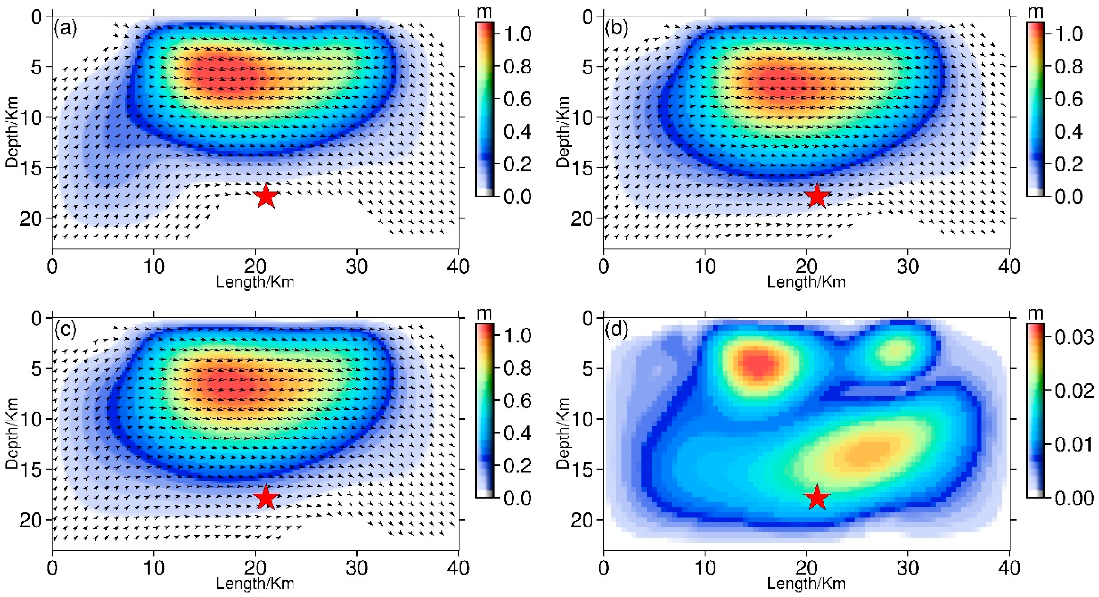
3.4. Characters of the Slip Distribution Model

The fault slip was mainly concentrated in a rectangular area 30 km long along the fault strike direction and 16 km wide along the dip direction, with a major slip at a depth of 1–15 km within the recoverable depth range of the checkerboard test, and one slip center at a depth of about 5–9 km (Figure 7c). The slip within the depth of 0–1 km was smaller than 0.25 m.

The maximum uncertainty of the slip model was about 3.2 cm (Figure 7d), equivalent to about 3.0% of its maximum slip (about 1.06 m). The average slip estimated by the MC method was about 0.28 ± 0.01 m, with an average rake angle about −7.86 ± 0.31°; the maximum slip was about 1.06 ± 0.02 m, located at a depth of 6.84 ± 0.33 km, with a rake angle about −10.37 ± 0.34°. When the shear modulus was μ = 32 GPa, the seismic moment was about (7.85 ± 0.13) × 10¹⁸ Nm, which was equivalent to a moment magnitude of about Mw 6.54 ± 0.01. The slip models showed that the Jiuzhaigou earthquake was a typical sinistral strike-slip rupture event.

4. Relationship between Fault Slip and Aftershocks

According to the precise location of aftershocks [34] during the month after the mainshock, the aftershocks were distributed over a zone of ~42 km with NWW–SEE trending about 150°, predominantly at a depth of 4–20 km. In addition, the dip angle of the seismogenic fault was steep with an average value of about 84°. Finally, the average positioning error of the aftershocks in the three directions of E–W, N–S, and U–D was 0.16, 0.15, and 0.18 km, respectively.

To reveal the relationship between the slip distribution and the aftershocks, we projected the positions of the aftershocks to the parallel and vertical direction of the fault trending, respectively (Figure 9). We found that there was a high consistency between the spatial distribution of the aftershocks and fault slip in the section parallel to the fault trending from NW to SE (Figure 9a). However, it is worth noting that the aftershocks were relatively scarce in the sliding peak center within the depth of 5–10 km, which may have been due to a full rupture of the mainshock in this region.

In addition, the fault geometric model essentially passed through the concentration zone of aftershocks in the section perpendicular to the fault trending from southwest (SW) to northeast (NE) (Figure 9b). There is also a need to note that the optimal dip angle of 77° was slightly smaller than that (~84°) directly suggested by the aftershocks [34]. From the multiple view geometries of the InSAR deformation fields (Figure 2), the deformation range and amplitude west of the fault were obviously larger than that in the east. In the case of a purely sinistral strike-slip rupture with vertical dip angle, the elastic deformation on both sides of the fault should be completely symmetrical. Apparently, the deformation of the Jiuzhaigou earthquake with a typical sinistral strike-slip rupture did not show symmetrical characteristics. Therefore, we suggest that the 77° dip angle was possibly more reasonable than the nearly vertical dip angle, considering the coincidence with the geodetic observation.

5. Stress Disturbance Due to the Jiuzhaigou Earthquake

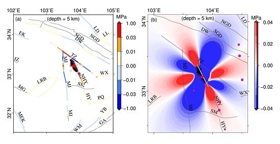
5.1. Coulomb Stress Change by the Mainshock

According to the seismic stress trigger theory, the fault rupture of an earthquake will always lead to stress disturbance at the epicenter and its surrounding zones. According to previous research [35,36,37], the stress change is perhaps highly correlated with the distribution of immediate aftershocks and has an effect on the seismic potentiality of the surrounding faults. According to the Coulomb failure criterion [38], the Coulomb stress is written as:

$${\sigma }_f={\tau }_{\beta }-\mu {\sigma }_{\beta }^{\prime },$$

(1)

where ${\sigma }_f$ is the Coulomb stress change on a specific receiving fault; ${\tau }_{\beta }$ (positive in the direction of fault slip) and ${\sigma }_{\beta }^{\prime }$ (positive in compression) are the shear stress and normal stress change on the receiving fault, respectively; $\mathsf{\mu }$ is the effective friction coefficient with a range 0–1. Using the fault slip distribution derived from the InSAR and GPS data, we calculated the coseismic Coulomb stress changes using the software package PSCMP/PSGRN [39]. The coseismic Coulomb stress changes with different depths of 0 to 20 km with an interval of 5 km were calculated using the optimal rupture plane of F1 with empirical friction of 0.4 for the receiving fault to reveal the triggering relationship between the mainshock and aftershocks (Figure 10).

The dislocation model is based on linear elasticity where only infinitesimal strain is assumed. In the vicinity of the rupturing surface, especially on their edges, an extremely large stress concentration occurs, and linear elasticity does not work. Due to the limitation of the dislocation model, the Coulomb stress changes in the near-field of the fault are unreliable; therefore, we do not discuss the spatial correlation between the near-field aftershocks and Coulomb stress changes.

The twenty-three aftershocks (M > 2) in the far-field of the fault within one year after the mainshock from 8 August 2017 to 7 July 2018 were compared with the Coulomb stress changes (Figure 10). We found that only five shocks occurred in the stress shadow area (Figure 10a–d), about 22% of the total number shocks in the far-field. Additionally, about 78% of the shocks happened in the positive stress change area, which were obviously consistent with the stress trigger theory. A notable phenomenon was that a total of eight shocks happened in the vicinity of the NHY fault (Figure 10).

To evaluate the effect of effective friction on the Coulomb stress changes, we also calculated the Coulomb stress changes with the frictions of 0.1 and 0.7 (Figures S2 and S3). The comparison showed that the different friction had a few influences on the Coulomb stress changes. However, the spatial correlation between the distribution of the off-fault aftershocks and Coulomb stress changes was not altered by the apparently different friction. Most of the aftershocks in the far-field happened in the positive stress change area with the different frictions.

5.2. Stress Disturbance at the Surrounding Faults

The Coulomb stress disturbances of the surrounding faults have been calculated in previous studies [7,40,41]. As our slip distribution model was somewhat different from previous models (Table 2), therefore, the stress disturbance to the surrounding faults due to the coseismic rupture needed to be reanalyzed for the receiving faults (Table S1). We not only considered the receiving faults [42], but also the Tazang fault and North Huya faults near the mainshock. The Tazang fault is considered as a southeastern extension of the East Kunlun fault. The North Huya fault is a hidden northern segment of the Huya fault. The strike direction, dip angle, and rake angle of the North Huya fault were assumed to be those of the mainshock fault model in the Section 3.2.

The stress distributions were calculated by the software PSCMP/PSGRN [39] with a stratified crustal model of Crust1.0. The stress distributions at the depth of 5 km showed that the remarkable stress increase (>0.1 MPa) at the Tazang fault was primarily located in the intersection with the Minjiang fault (Figure 11a). The stress increase of the Minjiang fault was localized west of the epicenter. The overall stress of the Huya fault was increased, especially in the northern hidden section, with a stress increase larger than 0.01 MPa. The stress disturbances to other faults were within ±0.01 MPa, approximate to the previous results [7,40,41]. The uncertainties of the stress distribution were also calculated based on the errors of the slip distribution model. Except for two small fragments in the middle-segment of the Tazang fault and the northern-segment of the north Huya fault (Figure 11b), most of the uncertainties were smaller than 0.003 MPa, which were within a reasonable range.

5.3. Seismic Potentiality of the Near-Field Fault

The static Coulomb stress was significantly enhanced (>0.01 MPa) in the northwestern Tazang fault that intersects with the Minjiang fault, with a static Coulomb stress increase at a segment more than 0.03 MPa, three times larger than the threshold to trigger future earthquakes. The static Coulomb stress also significantly increased in partial sections of the Minjiang fault, west of the epicenter with a maximum value of more than 0.03 MPa. However, the static Coulomb stress reduced in other sections of the Minjiang fault (Figure 11a). Therefore, this suggests that the Jiuzhaigou earthquake may increase the seismic potentiality of the northwestern section of the Tazang fault and partial sections of the Minjiang fault.

Some researchers have claimed that if the collective effect of the 2017 Jiuzhaigou Mw 6.5 earthquake, 1973 Huanglong M_W 6.5 earthquake, and the 1976 Songpan earthquake clusters break the Huya fault entirely from south to north, the seismic potentiality of the Huya fault may possibly be reduced [6,9]. However, other studies have found that the static Coulomb stress in the northern part of the Huya fault increased [40,43], and the latest activity of the Huya fault could possibly cause further earthquakes with a relatively small magnitude [11]. Our result confirmed a significant increase in the static Coulomb stress in the North Huya fault due to the Jiuzhaigou earthquake (Figure 11a).

6. Discussion

6.1. Comparison with Previous Slip Models

We collected the partly existing models of Ji et al. [7], Zhao et al. [9], Nie et al. [10], and Zhang et al. [12] and redrew them in the same color scales (Figure S4). A visual comparison of the models showed that there were some differences among them.

Our slip model showed that there was no significant slip in the lower left and right corners of the fault, which was different from previous models [7,9]. The maximum slip of our model was smaller than the model of Zhao et al. [9] and larger than the other models [7,10,12]. Unlike the other models, the seismic moment of our model was slightly larger than the focal mechanism solutions of GCMT and USGS (Table 2). Considering the role of aftershocks during the observation of the InSAR data, it would be reasonable to suggest that the seismic moments were slightly larger than the focal mechanism solution.

With the sole constraint of the geodetic data, the fault slip distribution models still differed from one another (Figure S4a–d). The discrepancies are possibly due to the fault geometric models. Our fault geometric parameters were derived from multiple view geometries of the InSAR data with nonlinear inversion methods, which were different from the previous studies [7,9,10,12]. We found that the fault geometry models retrieved by the nonlinear MPSO+MC and MCMC methods were highly consistent and the standard deviations of the fault geometry parameters were controlled within small values.

Overall, the fault slip distribution derived from the geodetic deformation measurements were principally located at the depth of 1–15 km (Figure S4a–d); whereas the addition of seismic waveform data caused dominant sliding to be located at a deeper depth (Figure S4e). Although there were some differences among the models, the dominant fault rake angles were all between –20° and 20°, indicating that the mainshock was attributable to a left-lateral strike-slip rupture.

6.2. Discrepancies of Coulomb Stress Changes of Mainshock Rupture

The coseismic Coulomb stress changes at the depth of 15 km, from the multiple coseismic slip distribution models, were calculated with the same crustal model, and receiving fault of the mainshock rupture (Figure S5) to evaluate the influence of the coseismic slip distribution models to the static Coulomb stress changes. We found some discrepancies in the coseismic Coulomb stress changes.

Coulomb stress distributions are obviously different from each other in the near-field of the fault (Figure S5). If we hypothesize that the nonlinear elastic actions in the vicinity of fault are similar, the discrepancies in the five dislocation models may dominantly influence the Coulomb stress distributions in the near-field of the fault. There were also some diversities in the far-field of the fault; however, these diversities will not influence the spatial correlation comparison between the far-field aftershock and Coulomb stress change (Figure S5).

It is noteworthy that if we ignored the nonlinear elastic action in the vicinity of the fault, the discrepancy of the existing coseismic slip distribution models may bias the spatial relationship analysis of the near-field aftershocks with static Coulomb stress changes. For example, the near-field aftershocks at the depth range of 15–20 km occurred mostly in the positive Coulomb stress area identified with the models of Zhao et al. [9], Zhang et al. [12], and this work (Figure S5a,b,e). However, they happened mostly in the shadow area with the models of Ji et al. [7] and Nie et al. [10] (Figure S5c,d).

6.3. Discrepancies of Coulomb Stress Disturbance to Nearby Faults

Using the different slip distribution models (Figure S4), the stress disturbances to nearby faults at the depth of 5 km were calculated by the software PSCMP/PSGRN with the same crustal model and receiving faults (Table S1). We found that the differences of the coseismic slip distribution models may bias the Coulomb stress disturbances to nearby faults (Figure S6). The magnitude of positive stress changes at the MJ fault west of the epicenter was larger than 0.03 MP using the slip models of Nie et al. [10] and this work (Figure S6a,d). Whereas, it was smaller than 0.03 MPa with the slip models of Ji et al. [7], Zhao et al. [9], and Zhang et al. [12] (Figure S6b,c,e). The positive stress perturbations to the Tazang fault east of the epicenter were not significant when calculated with the slip models of Ji et al. [7], Zhao et al. [9], and this study—however, they were significant based on the estimate obtained from the slip model of Nie et al. [10] and Zhang et al. [12].

7. Conclusions

We inverted for the seismogenic fault geometry models of the Jiuzhaigou Mw 6.5 earthquake from InSAR data by the MPSO+MC and MCMC nonlinear algorithms, and the slip distribution by the SDM+MC method. The fault geometry and slip model were compared with the distribution of the relocated aftershocks. Then, the static Coulomb stress disturbances to the mainshock rupture plane and nearby faults were analyzed. Finally, the discrepancies of several existing slip distribution models and Coulomb stress changes due to the slip models were discussed. The main findings were as follows:

(1)

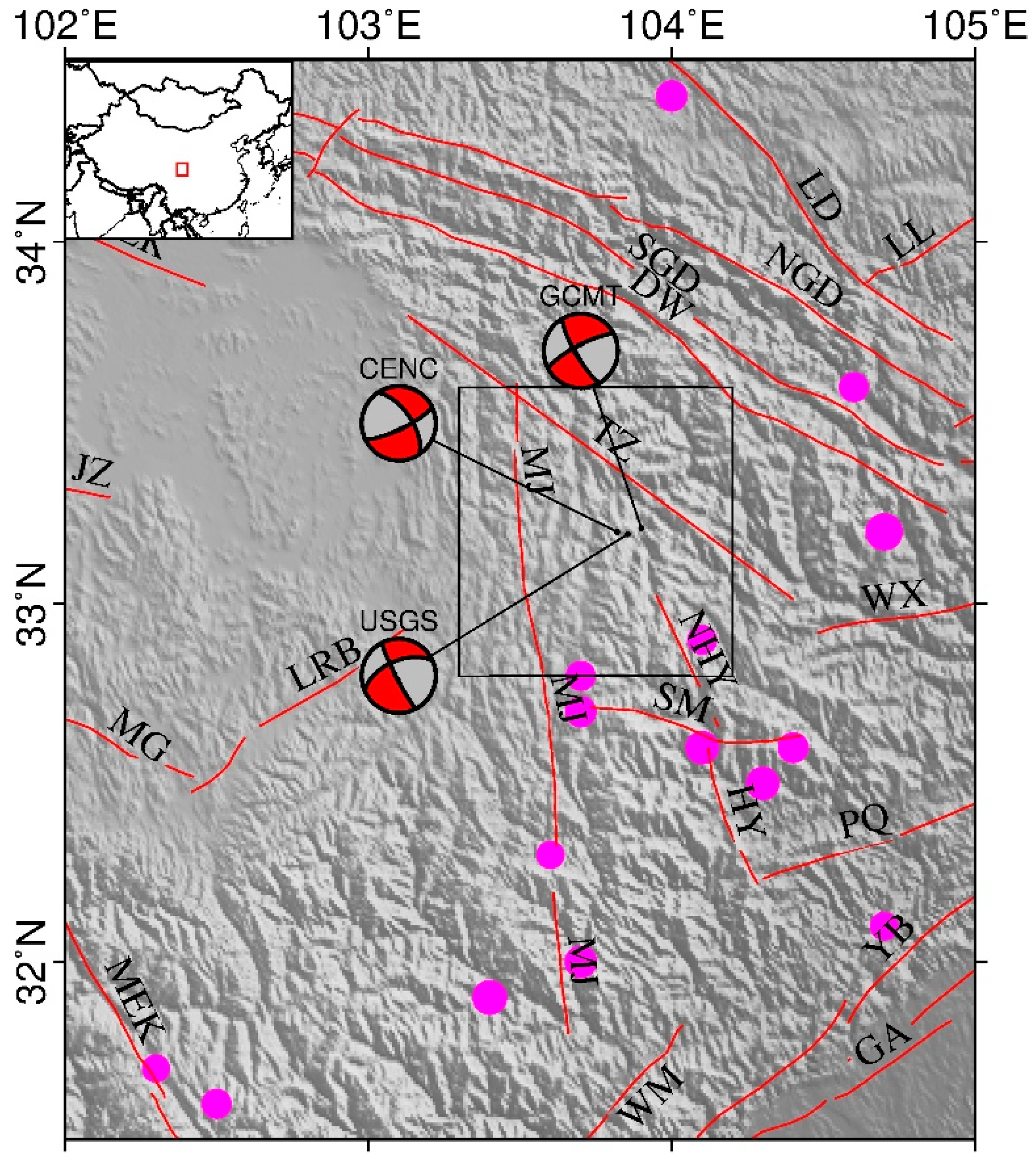
A blind faulting with a length of about 23 km, a width of about 11 km, a strike angle of about 154°, an optimized dip angle of 77°, was causative of the Jiuzhaigou earthquake.

(2)

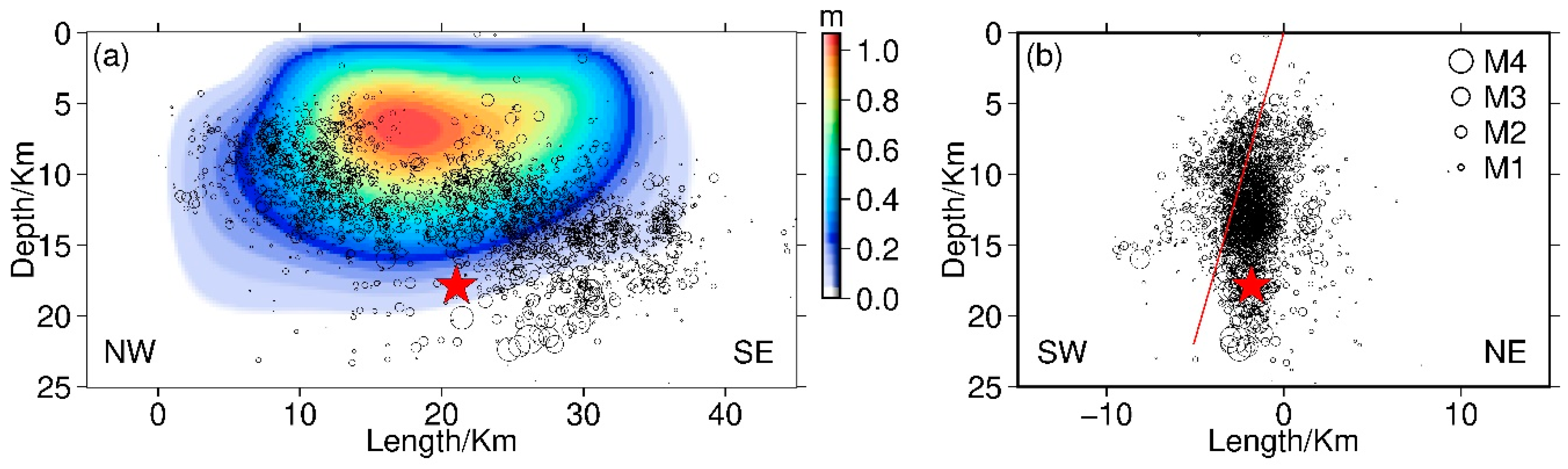
The fault slip was majorly concentrated at the depth of 1–15 km, and only one slip center appeared at the depth of 5–9 km with a maximum slip of ~1.06 m. The average rake angle was about 7.84°, indicating the pure left-lateral strike-slip fracture of the mainshock.

(3)

The seismic moment derived from the slip distribution was about 7.85 × 10¹⁸ Nm, equivalent to a moment magnitude about Mw 6.54, which was slightly larger than the previous results and the focal mechanism solutions.

(4)

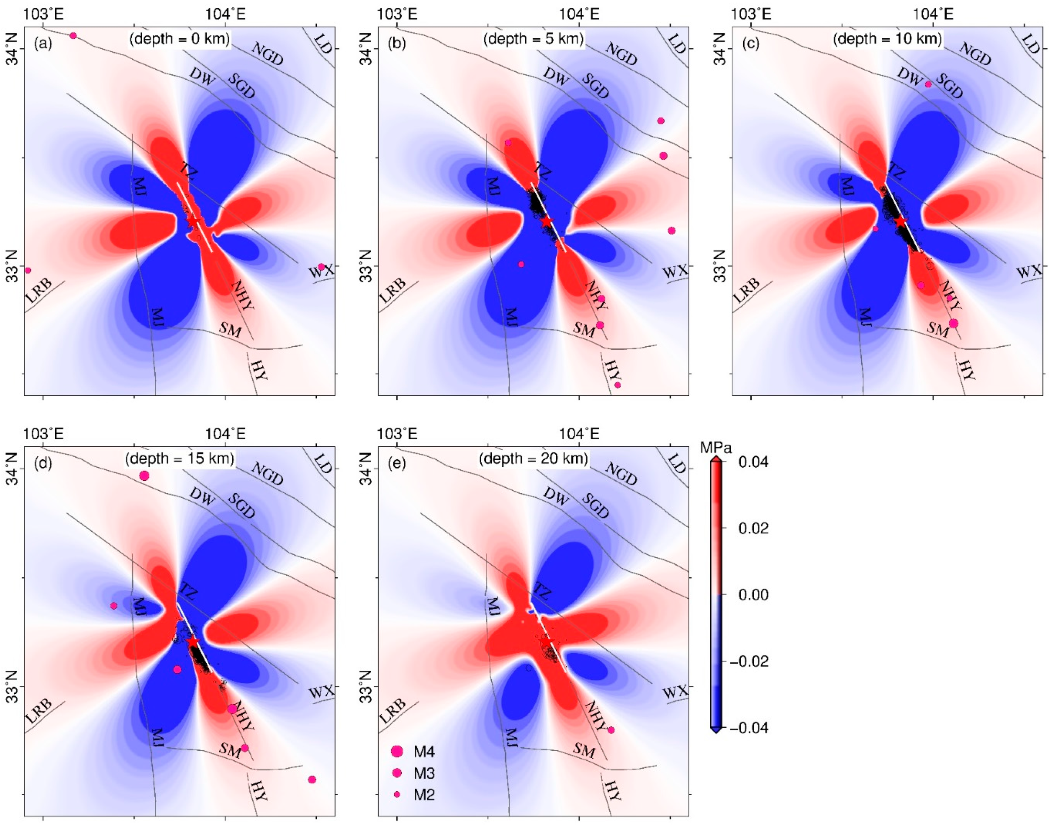
Most of the off-fault aftershocks with the magnitude >M 2 within one year after the mainshock happened in the stress positive stress change area, which coincided with the stress triggering theory.

(5)

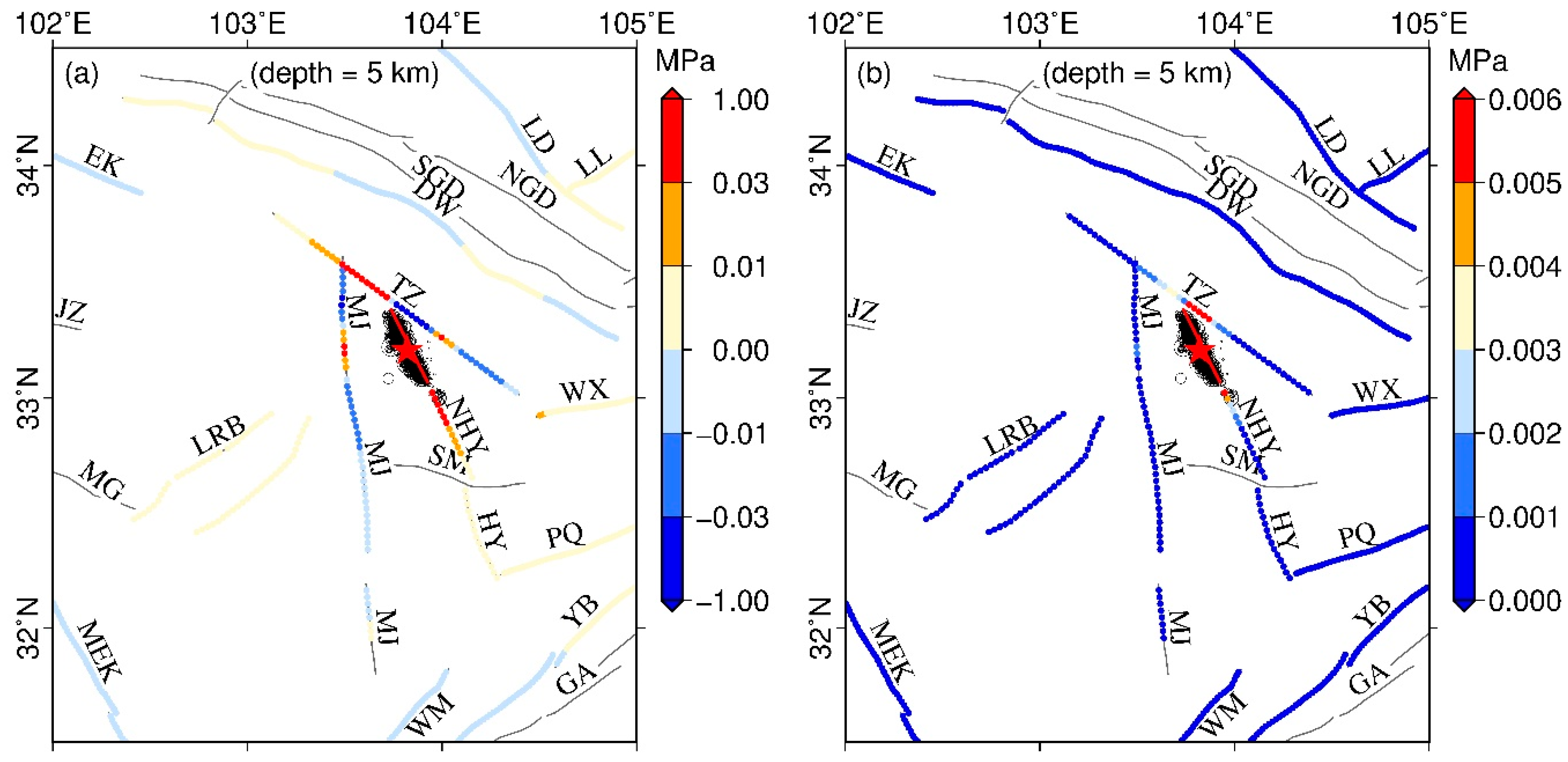
The Coulomb stress obviously increased (>0.01 MPa) in the northwestern section of the Tazang fault, a partial segment of the Minjiang fault west of the epicenter, and the hidden North Huya fault, where the seismic potentiality was possibly enhanced.

References

1. Wang, K.; Shen, Z.K. Location and focal mechanism of the 1933 Diexi earthquake and its associated regional tectonics. Acta Seismol. Sin. 2011, 33, 557–567. (In Chinese) [Google Scholar]
2. Zhu, H.; Wen, X.Z. Stress triggering process of the 1973 to 1976 Songpan, Sichuan, Sequence of strong earthquakes. Chin. J. Geophys. 2009, 52, 994–1003. (In Chinese) [Google Scholar] [CrossRef]
3. Chen, S.F.; Wilson, C.J.L.; Deng, Q.D.; Zhao, X.L. Active faulting and block movement associated with large earthquakes in the Min Shan and Longmen Mountains, northeastern Tibetan Plateau. J. Geophys. Res. Solid Earth 1994, 99, 24025–24038. [Google Scholar] [CrossRef]
4. Xu, X.W.; Chen, G.H.; Wang, Q.X.; Chen, L.C.; Ren, Z.K.; Xu, C.; Wei, Z.Y.; Lu, R.Q.; Tan, X.B.; Dong, S.P.; et al. Discussion on seismogenic structure of Jiuzhaigou earthquake and its implication for current strain state in the southeastern Qinghai-Tibet Plateau. Chin. J. Geophys. 2017, 60, 4018–4026. (In Chinese) [Google Scholar] [CrossRef]
5. Yang, Y.H.; Fan, J.; Hua, Q.; Gao, J.; Wang, C.L.; Zhou, L.; Zhao, T. Inversion for the focal mechanisms of the 2017 Jiuzhaigou M7.0 earthquake sequence using near-field full waveforms. Chin. J. Geophys. 2017, 60, 4098–4104. (In Chinese) [Google Scholar] [CrossRef]
6. Shan, X.J.; Qu, C.Y.; Gong, W.Y.; Zhao, D.Z.; Zhang, Y.F.; Zhang, G.H.; Song, X.G.; Liu, Y.H.; Zhang, G.F. Coseismic deformation field of the Jiuzhaigou Ms7.0 earthquake from Sentinel-1A InSAR data and fault slip inversion. Chin. J. Geophys. 2017, 60, 4527–4536. (In Chinese) [Google Scholar] [CrossRef]
7. Ji, L.Y.; Liu, C.J.; Xu, J.; Liu, L.; Long, F.; Zhan, Z.W. InSAR observation and inversion of the seismogenic fault for the 2017 Jiuzhaigou MS 7.0 earthquake in China. Chin. J. Geophys. 2017, 60, 4069–4082. (In Chinese) [Google Scholar] [CrossRef]
8. Wang, Y.B.; Gan, W.J.; Chen, W.T.; You, X.Z.; Liang, W.P. Coseismic displacements of the 2017 Jiuzhaigou M7.0 earthquake observed by GNSS: Preliminary results. Chin. J. Geophys. 2018, 61, 161–170. (In Chinese) [Google Scholar] [CrossRef]
9. Zhao, D.; Qu, C.; Shan, X.; Gong, W.; Zhang, Y.; Zhang, G. InSAR and GPS derived coseismic deformation and fault model of the 2017 Ms7.0 Jiuzhaigou earthquake in the Northeast Bayanhar block. Tectonophysics 2018, 726, 86–99. [Google Scholar] [CrossRef]
10. Nie, Z.; Wang, D.-J.; Jia, Z.; Yu, P.; Li, L. Fault model of the 2017 Jiuzhaigou Mw6.5 earthquake estimated from coseismic deformation observed using Global Positioning System and Interferometric Synthetic Aperture Radar data. Earth Planets Space 2018, 70. [Google Scholar] [CrossRef]
11. Sun, J.; Yue, H.; Shen, Z.; Fang, L.; Zhan, Y.; Sun, X. The 2017 Jiuzhaigou earthquake: A complicated event occurred in a young fault system. Geophys. Res. Lett. 2018, 45. [Google Scholar] [CrossRef]
12. Zhang, X.; Feng, W.P.; Xu, L.S.; Li, C.L. The source-process inversion and the intensity estimation of the 2017 Ms7.0 Jiuzhaigou earthquake. Chin. J. Geophys. 2017, 60, 4105–4116. (In Chinese) [Google Scholar] [CrossRef]
13. Feng, W.P.; Li, Z.H. A novel hybrid PSO/simplex algorithm for determining earthquake source parameters using InSAR data. Progress Geophys. 2010, 25, 1189–1196. (In Chinese) [Google Scholar] [CrossRef]
14. Parsons, B.; Wright, T.; Rowe, P.; Andrews, J.; Jackson, J.; Walker, R.; Khatib, M.; Talebian, M.; Bergman, E.; Engdahl, E.R. The 1994 Sefidabeh (eastern Iran) earthquakes revisited: new evidence from satellite radar interferometry and carbonate dating about the growth of an active fold above a blind thrust fault. Geophys. J. Int. 2006, 164, 202–217. [Google Scholar] [CrossRef] [Green Version]
15. Zhou, X. Markov Chain Monte Carlo method used to invert for fault slip from geodetic data. J. Geod. Geodyn. 2017, 37, 996–1002. (In Chinese) [Google Scholar] [CrossRef]
16. Wang, R.; Diao, F.; Hoechner, A. SDM—A geodetic inversion code incorporating with layered crust structure and curved fault geometry. EGU Gen. Assem. 2013, 15, EGU2013–2411. [Google Scholar]
17. Rosen, P.A.; Gurrola, E.; Sacco, G.F.; Zebker, H. The InSAR scientific computing environment. In Proceedings of the 2012 EUSAR. 9th European Conference on Synthetic Aperture Radar, Nürnberg, Germany, 23–26 April 2012; pp. 730–733. [Google Scholar]
18. Farr, T.G.; Rosen, P.A.; Caro, E.; Crippen, R.; Duren, R.; Hensley, S.; Kobrick, M.; Paller, M.; Rodriguez, E.; Roth, L.; et al. The Shuttle Radar Topography Mission. Rev. Geophys. 2007, 45, RG2004. [Google Scholar] [CrossRef]
19. Chen, C.W.; Zebker, H.A. Phase unwrapping for large SAR interferograms: Statistical segmentation and Generalized network models. IEEE Trans. Geosci. Remote Sens. 2002, 40, 1709–1719. [Google Scholar] [CrossRef]
20. Yague-Martinez, N.; Prats-Iraola, P.; Rodriguez Gonzalez, F.; Brcic, R.; Shau, R.; Geudtner, D.; Eineder, M.; Bamler, R. Interferometric processing of Sentinel-1A TOPS data. IEEE Trans. Geosci. Remote Sens. 2016, 54, 2220–2234. [Google Scholar] [CrossRef]
21. Rodriguez, E.; Morris, C.S.; Belz, J.E.; Chapin, E.C.; Martin, J.M.; Daffer, W.; Hensley, S. An Assessment of the SRTM Topographic Products; Technical Report JPL D-31639; Jet Propulsion Laboratory: Pasadena, CA, USA, 2005. [Google Scholar]
22. Gray, A.L.; Mattar, K.E.; Sofko, G. Influence of ionospheric electron density fluctuations on satellite radar interferometry. Geophys. Res. Lett. 2000, 27, 1451–1454. [Google Scholar] [CrossRef] [Green Version]
23. Yu, C.; Li, Z.; Penna, N.T. Interferometric synthetic aperture radar atmospheric correction using a GPS-based iterative tropospheric decomposition model. Remote Sens. Environ. 2018, 204, 109–121. [Google Scholar] [CrossRef]
24. Yu, C.; Penna, N.T.; Li, Z. Generation of real-time mode high-resolution water vapor fields from GPS observations. J. Geophys. Res. Atmos. 2017, 122, 2008–2025. [Google Scholar] [CrossRef] [Green Version]
25. Lohman, R.B.; Simons, M. Some thoughts on the use of InSAR data to constrain models of surface deformation: Noise structure and data downsampling. Geochem. Geophys. Geosyst. 2005, 6, Q01007. [Google Scholar] [CrossRef]
26. Li, Z.; Elliott, J.; Feng, W.; Walters, R. The 2010 MW 6.8 Yushu (Qinghai, China) earthquake: Constraints provided by InSAR and body wave seismology. J. Geophys. Res. 2011, B10302. [Google Scholar] [CrossRef]
27. Feng, W.; Li, Z.; Elliott, J.R.; Fukushima, Y.; Hoey, T.; Singleton, A.; Cook, R.; Xu, Z. The 2011 Mw 6.8 Burma earthquake: fault constraints provided by multiple SAR techniques. Geophys. J. Int. 2013, 195, 650–660. [Google Scholar] [CrossRef]
28. Yabuki, T.; Matsu’ura, M. Geodetic data inversion using a Bayesian information criterion for spatial distribution of fault slip. Geophys. J. Int. 1992, 109, 363–375. [Google Scholar] [CrossRef] [Green Version]
29. Fukuda, J.; Johnson, K.M. A Fully Bayesian Inversion for Spatial Distribution of Fault Slip with Objective Smoothing. Bull. Seismol. Soc. Am. 2008, 98, 1128–1146. [Google Scholar] [CrossRef]
30. Diao, F.; Xiong, X.; Wang, R.; Zheng, Y.; Walter, T.R.; Weng, H.; Li, J. Overlapping post-seismic deformation processes: Afterslip and viscoelastic relaxation following the 2011 mw 9.0 Tohoku (Japan) earthquake. Geophys. J. Int. 2014, 196, 218–229. [Google Scholar] [CrossRef]
31. Bie, L.; Hicks, S.; Garth, T.; Gonzalez, P.; Rietbrock, A. ‘Two go together’: Near-simultaneous moment release of two asperities during the 2016 Mw 6.6 Muji, China earthquake. Earth Planet. Sci. Lett. 2018, 491, 34–42. [Google Scholar] [CrossRef]
32. Laske, G.; Masters, G.; Ma, Z.; Pasyanos, M. Update on CRUST1.0—A 1-degree Global Model of Earth’s Crust. Geophys. Res. Abstr. 2013, 15, EGU2013–2658. [Google Scholar]
33. Wang, R.; Martín, F.L.; Roth, F. Computation of deformation induced by earthquake in a multi-layered elastic crust-FORTRAN programs EDGRN/EDCMP. Comput. Geosci. 2003, 29, 195–207. [Google Scholar] [CrossRef]
34. Fang, L.H.; Wu, J.P.; Su, J.R.; Wang, M.M.; Jiang, C.; Fan, L.P.; Wang, W.L.; Wang, C.Z.; Tan, X.L. Relocation of mainshock and aftershock sequence of the Ms7.0 Sichuan Jiuzhaigou earthquake. China Sci. Bull. 2018, 63, 649–662. [Google Scholar] [CrossRef]
35. Toda, S.; Stein, R.S.; Reasenberg, P.A.; Dieterich, J.H.; Yoshida, A. Stress transferred by the 1995 Mw = 6.9 kobe, Japan, shock: effect on aftershocks and future earthquake probabilities. J. Geophys. Res. Solid Earth 1998, 103, 24543–24565. [Google Scholar] [CrossRef]
36. McCloskey, J.; Nalbant, S.S.; Steacy, S.; Nostro, C.; Scotti, O.; Baumont, D. Structural constrains on the spatial distribution of aftershocks. Geophys. Res. Lett. 2005, 30, 1610. [Google Scholar] [CrossRef]
37. De Natale, G.; Crippa, B.; Troie, C.; Pingue, F. Abruzzo, Italy, earthquakes of April 2009: heterogeneous fault-slip models and stress transfer from accurate inversion of ENVISAT-InSAR data. Bull. Seismol. Soc. Am. 2011, 101, 2340–2354. [Google Scholar] [CrossRef]
38. Ross, S.S.; Aykut, A.B.; James, H.D. Progressive failure on the North Anatolian fault since 1939 by earthquake stress triggering. Geophys. J. Int. 1997, 128, 594–604. [Google Scholar] [Green Version]
39. Wang, R.J.; Lorenzo-Martin, F.; Roth, F. PSGRN/PSCMP-a new code for calculation co- and post-seismic deformation, geoid and gravity changes based on the viscoelastic-gravitational dislocation theory. Comput. Geosci. 2006, 32, 527–541. [Google Scholar] [CrossRef]
40. Shan, B.; Zheng, Y.; Liu, C.L.; Xie, Z.J.; Kong, J. Coseismic Coulomb failure stress changes caused by the 2017 M7.0 Jiuzhaigou earthquake, and its relationship with the 2008 Wenchuan earthquake. Sci. China Earth Sci. 2017, 47, 1329–1338. [Google Scholar] [CrossRef]
41. Xu, J.; Shao, Z.G.; Liu, J.; Ji, L.Y. Analysis of interaction between great earthquakes in the eastern Bayan Har block based on changes of Coulomb stress. Chin. J. Geophys. 2017, 60, 4056–4068. (In Chinese) [Google Scholar] [CrossRef]
42. Xu, J.; Shao, Z.G.; Ma, H.S.; Zhang, L.P. Impact of the 2008 Wenchuan 8.0 and 2013 Lushan 7.0 earthquakes along the Longmenshan fault zone on surrounding faults. Earthquake 2014, 34, 40–49. (In Chinese) [Google Scholar]
43. Wang, J.J.; Xu, C.J. Coseismic Coulomb stress changes associated with the 2017 Mw6.5 Jiuzhaigou earthquake (China) and its impacts on surrounding major faults. Chin. J. Geophys. 2017, 60, 4398–4420. (In Chinese) [Google Scholar] [CrossRef]
Figure 1. The regional tectonic of Jiuzhaigou earthquake. Abbreviations are: East Kunlun fault = EKL, Tazang fault = TZ, Minjiang fault = MJ, Huya fault = HY, North Huya fault = NHY, Snow Mountain fault = SM, Pingwu–Qingchuan fault = PQ, WenXian fault = WX, Yingxiu–Beichuan fault = YB, Wenchuan–Maowen fault = WM, Maerkang fault = MEK, Maduo–Gande fault = MG, Jiuzhi fault = JZ, Guanxian–Anxian fault = GA, Diebu–Whitelongjang fault = DW, South Guankaishan–Dieshan fault = SGD, North Guankaishan–Dieshan fault = NGD, Lintan–Dangchang fault = LD, Lixian–Luojiapu fault = LL. The purple solid circles are the earthquakes that were larger than M 6 according to the CSI. The black rectangle is the InSAR measurement region in this study. The focal mechanism solutions are from the USGS, GCMT and CSI.
Remotesensing 10 01400 g001
Figure 2. The InSAR coseismic deformation fields. (ac) Corresponding coseismic deformation fields of the interferogram pairs of S1A, S1D and R2A, respectively.
Remotesensing 10 01400 g002
Figure 3. The comparison of the R_Based and Quadtree down-sampling. (a,b) R_Based and Quadtree down-sampling of the coseismic deformation field of R2A, respectively. The density of noisy points in the far field decreased sharply with the R_Based method.
Remotesensing 10 01400 g003
Figure 4. The mean values (µ) and standard deviation (ξ) of the fault parameters calculated by the MC method.
Remotesensing 10 01400 g004
Figure 5. The marginal probability density function of fault geometry parameters calculated by the Markov Chain Monte Carlo (MCMC) algorithm.
Remotesensing 10 01400 g005
Figure 6. The method of deciding the smooth factor and dip angle. (a) Trade-off curve of the relative fitting residuals of Misfit and the logarithm of Roughness; the asterisk is the position of the smoothness factor used. (b) Trade-off curve between the RMS Misfit and dip angle; the asterisk is the position of the dip angle adopted to invert for the slip distribution. The Misfit was subtracted by 0.284 in plot (b).
Remotesensing 10 01400 g006
Figure 7. The slip distributions and uncertainties derived from the steepest descent method + Monte Carlo (SDM+MC) inversion. (a) Slip distribution inverted only based on the Sentinel-1A/B data; (b) Slip distribution inverted based on the combination of the Sentinel-1A/1B and Radarsat-2 data, which the slip distribution in the lower left is more reasonable than (a); (c) Slip distribution inverted based on the combination of the Sentinel-1A/1B, Radarsat-2, and GPS data, which was the optimum solution with the S1 model in Table 2; (d) Uncertainties with the slip distribution of the S1 model. The maximum uncertainty of the fault sliding was about 3.2 cm. The maximal fault sliding was about 1.06 m. The red pentagram is the mainshock by Fang et al. [34].
Remotesensing 10 01400 g007
Figure 8. The deformation residuals of the distributed slip model. (ac) The InSAR residuals of S1A, S1D, and R2A, respectively; (d) Red and blue arrows are the observation and simulation deformation of GPS, separately. The red solid line is the fault model of S1 in the surface. The maximal residuals were smaller than 0.1 m and the mean residuals were separately 1.9 cm, 1.4 cm, and 0.8 cm for the S1A, S1D, and R2A. The simulation deformations of GPS were generally consistent with the observations with a mean residual of about 2.0 mm.
Remotesensing 10 01400 g008
Figure 9. The spatial distribution of relocated aftershocks and fault slip model. (a) Section parallel to the strike of the fault from northwest (NW) to southeast (SE); (b) Section perpendicular to the strike of the fault from SW to NE. The relocated aftershocks denoted by black circles and the mainshock by the red pentagram are from Fang et al. [34]; the slip distribution model is S1; the red line is the fault location in the section. The fault geometry and slip distribution had a high consistency with the aftershocks.
Remotesensing 10 01400 g009
Figure 10. Coseismic Coulomb stress changes with the receiving fault of the mainshock rupture (i.e., strike = 154°, dip = 77°, rake = –8°, friction = 0.4). (ae) Coulomb stress changes in the depth of 0 km, 5 km, 10 km, 15 km and 20 km, respectively. The white line is the optimal fault model of this work. The near-field relocated aftershocks denoted by black circles and the mainshock by a red pentagram are from Fang et al. [34]. The far-field aftershocks denoted by rose-red solid circles are from CSI. The magnitude of near-field aftershocks is referred to in Figure 9b. The gray lines are faults referred to in Figure 1. The depth of the aftershocks is <5 km with a, ≥5 km and <10 km with b, ≥10 km and <15 km with c, ≥15 km and <20 km with d, and ≥20 km with e, respectively.
Remotesensing 10 01400 g010
Figure 11. The coseismic Coulomb stress distributions and uncertainties in the surrounding faults at the depth of 5 km. (a) Coseismic Coulomb stress distributions; (b) Uncertainties of the coseismic Coulomb stress distributions. The Coulomb stress obviously increased in the northwest section of the Tazang fault, the partial segments of the Minjiang fault just west of the epicenter, and the hidden North Huya fault. The red line is the fault model of S1 on the surface. The black points and red pentagram are separately the relocated aftershocks and mainshock from Fang et al. [34]. The fault names are referred to in Figure 1 and the fault parameters are referred to in Table S1.
Remotesensing 10 01400 g011