An Improved Spatial and Temporal Reflectance Unmixing Model to Synthesize Time Series of Landsat-Like Images

Abstract

The trade-off between spatial and temporal resolution limits the acquisition of dense time series of Landsat images, and limits the ability to properly monitor land surface dynamics in time. Spatiotemporal image fusion methods provide a cost-efficient alternative to generate dense time series of Landsat-like images for applications that require both high spatial and temporal resolution images. The Spatial and Temporal Reflectance Unmixing Model (STRUM) is a kind of spatial-unmixing-based spatiotemporal image fusion method. The temporal change image derived by STRUM lacks spectral variability and spatial details. This study proposed an improved STRUM (ISTRUM) architecture to tackle the problem by taking spatial heterogeneity of land surface into consideration and integrating the spectral mixture analysis of Landsat images. Sensor difference and applicability with multiple Landsat and coarse-resolution image pairs (L-C pairs) are also considered in ISTRUM. Experimental results indicate the image derived by ISTRUM contains more spectral variability and spatial details when compared with the one derived by STRUM, and the accuracy of fused Landsat-like image is improved. Endmember variability and sliding-window size are factors that influence the accuracy of ISTRUM. The factors were assessed by setting them to different values. Results indicate ISTRUM is robust to endmember variability and the publicly published endmembers (Global SVD) for Landsat images could be applied. Only sliding-window size has strong influence on the accuracy of ISTRUM. In addition, ISTRUM was compared with the Spatial Temporal Data Fusion Approach (STDFA), the Enhanced Spatial and Temporal Adaptive Reflectance Fusion Model (ESTARFM), the Hybrid Color Mapping (HCM) and the Flexible Spatiotemporal DAta Fusion (FSDAF) methods. ISTRUM is superior to STDFA, slightly superior to HCM in cases when the temporal change is significant, comparable with ESTARFM and a little inferior to FSDAF. However, the computational efficiency of ISTRUM is much higher than ESTARFM and FSDAF. ISTRUM can to synthesize Landsat-like images on a global scale.

1. Introduction

Landsat images have the longest continuous record of the Earth surface with fine resolution of 30 m (denoted by fine-resolution image henceforth). It has been widely applied by the scientific community [1]. However, due to the trade-off between spatial and temporal resolution, Landsat sensor revisits the same region every 16 days, which limits its applicability in studies. For example, fine-resolution vegetation phenology mapping [2] and crop type mapping [3] require both high spatial and temporal resolution images. For regions with frequent cloud contamination, the time interval may be longer to achieve an image that can be used to extract information on the instantaneous field of view [4]. To overcome this constraint, spatiotemporal image fusion methods have been developed to synthesize time series of Landsat-like images by blending low spatial resolution but high temporal resolution images (henceforth denoted by coarse-resolution image) such as the MODerate resolution Imaging Spectroradiometer (MODIS) and the Medium Resolution Imaging Spectrometer (MERIS) [5,6,7,8,9,10,11,12]. In the remote sensing image fusion domain, spatiotemporal fusion is different from the superresolution methods which enhance the spatial resolution by combining single-frame or multi-frame images [13], and different from the pansharpening methods (referred to as spatial-spectral fusion) which enhance the spatial resolution and retain spectral resolution of multi-spectral bands with a simultaneously acquired panchromatic band [14]. Spatiotemporal fusion methods aim to generate fine-resolution images with frequent temporal coverage [15]. Inputs of these methods are one or more Landsat and coarse-resolution image pairs (L-C pairs) observed on the same dates (henceforth denoted by base date, $T_B$), and one coarse-resolution image observed on the prediction date ($T_P$). Output is a Landsat-like image on $T_P$, which captures the temporal change during $T_B$ and $T_P$ and retains the spatial details. The synthetic time series Landsat-like images have been effectively applied in vegetation monitoring [16,17], crop types mapping [18], fine-resolution land surface temperature monitoring [19,20], daily evapotranspiration mapping [21,22], and water environment monitoring [23,24].

Typically, in technical literature, the spatiotemporal image fusion methods can be categorized into five types [15]: spatial-unmixing based, weight-function based, learning based, Bayesian based, and hybrid methods. The method proposed by Zurita-Milla et al. [6], the STDFA [25] and the STRUM [26] are typical spatial-unmixing based methods. The theoretical basis of these methods is linear spectral mixture of coarse pixels [6]. Different from the spectral-unmixing, which computes the abundance with known spectra of endmembers, spatial-unmixing computes the spectra of endmembers with known abundance. Spatial-unmixing based methods have the advantage of retrieving accurate spectra of endmembers [27]. However, their shortcoming is the synthetic image lacks intra-class spectral variability and spatial details [27]. Because the methods assume each fine pixel contains only one class type and the computed spectra of endmembers are directly assigned to a class image to synthesize the fine-resolution image [6]. The spatial and temporal adaptive reflectance fusion model (STARFM) [5], the Enhanced STARFM (ESTARFM) [7], and the spatial and temporal nonlocal filter-based fusion model (STNLFFM) [28] are typical weight-function based methods. A fine pixel value is estimated by weighting the information of its surrounding similar pixels in these methods. Spatial details are better retained than spatial-unmixing based methods. However, the spectral mixture of coarse pixels are not taken into account in the weighted model [27]. Learning-based methods generally contain two processes, i.e., the learning and applying of the model [15]. Dictionary-pair learning [8,9], regression tree [29], and deep convolutional network [30] have been adopted in learning-based methods with good performance. However, selection of learning samples has significant influence on the accuracy of learning-based methods, and the computation expense is also high to train a model [31]. Some relatively simple but efficient learning-based methods were also proposed. Hazaymeh and Hassan [32,33] proposed a spatiotemporal image-fusion model (STI-FM) which builds the relationship between coarse-resolution images observed on $T_B$ and $T_P$, and applies the model to Landsat image on $T_B$ to synthesize Landsat-like image. STI-FM is capable of enhancing the temporal resolution of both land surface temperature and reflectance images of Landsat-8. Kwan et al. [34,35] proposed the HCM which first learns a pixel-to-pixel transformation matrix based on coarse-resolution images and then applies the matrix to Landsat image. Both STI-FM and HCM are simple and computationally efficient with high performance [34]. Bayesian based methods synthesize images in a probabilistic manner based on the Bayesian estimation theory. By making use of the advantage of multivariate arguments, it is flexible to predict temporal changes [36]. However, fusion accuracy is sensitive to the model assumptions and parameter estimations. Spectral mixture of coarse pixels is also not fully incorporated in the methods [36]. By combining advantages of two or more methods of the above four categories, hybrid methods were proposed [15]. The FSDAF [10] is a typical hybrid method. It performs temporal and spatial predictions by spatial-unmixing and Thin Plate Spline (TPS) interpolator separately, and combines two predictions with the idea of weight-function based methods. Hybrid methods could be more flexible in dealing with complicated scenarios, e.g., heterogeneous landscapes [37], abrupt land cover type changes [10] and shape changes [12]. However, accuracy improvement is at the cost of complicated processing steps and computational expense.

Spatiotemporal image fusion methods should capture temporal change of land surface. Because land surface changes in different ways across different regions and periods, each fusion method may have its own suitable situations [26]. There is probably no universally best method. Simple methods can outperform complicated methods if the conditions are suitable [38]. It is valuable to diversify the fusion methods to give more choices in applications [34]. It is also meaningful to improve existing fusion methods. Aiming to fix the shortcoming of the spatial-unmixing based method proposed by Zurita-Milla et al. [6], Gevaert and García-Haro [26] proposed STRUM. Different from the method proposed by Zurita-Milla et al. [6] which directly performs the spatial-unmixing to coarse-resolution image on $T_P$, STRUM first calculates a coarse-resolution temporal change image by subtracting coarse-resolution image on $T_B$ from the image on $T_P$. Then, the difference image is disaggregated by spatial-unmixing to synthesize the fine-resolution temporal change image, which is further added to Landsat image on $T_B$ to synthesize Landsat-like image on $T_P$. Therefore, the synthetic image inherits spectral variability and spatial details from Landsat image on $T_B$ to some degree [26]. The STRUM outperforms STARFM and original spatial-unmixing method, even when there are few reference Landsat images [26]. However, because classification image is applied in spatial-unmixing process, the downscaled fine-resolution temporal change image in STRUM still lacks intra-class spectral variability and spatial details.

Because of the heterogeneity of land surface, more than one land cover types could exist in a Landsat pixel at the scale of 30 m. Mixed pixels commonly occur in Landsat image [39]. The hard-classification image is unable to represent the varied combinations of endmembers in the pixels [39]. Generally, land surface varies gradually even on the boundaries of different land cover types. The abundance image, which records area fractions of endmembers in the pixel, could report continuous gradations and retain the spatial structure of land surface, thus providing a more accurate representation of land surface than class image [39]. Therefore, it is more appropriate to mix spectra of endmembers with fine-resolution abundance image than to assign it to classification image. For the reasons above, we proposed Improved STRUM (ISTRUM) by taking advantages of abundance images in order to tackle the aforementioned shortcoming of STRUM. By surveying the studies on the spatial-unmixing based methods [6,25,26,40,41], we found that ISTRUM is the first study that applies fine-resolution abundance image in spatial-unmixing process. In STRUM, the derived fine-resolution temporal change image based on coarse-resolution image is directly added to Landsat image. The sensor difference between Landsat and coarse-resolution imaging systems is not considered [26]. It was adjusted with a linear model in ISTRUM. Moreover, STRUM only considered the situation when only one L-C image pair is available [26]. A method to combine results synthesized by multiple L-C pairs was integrated in ISTRUM in order to enhance its applicability for situations when multiple L-C pairs are available.

The objective of this paper is: (1) to describe the framework of ISTRUM; (2) to evaluate the performance improvement of ISTRUM by comparing it with STRUM; (3) to analyze the sensitivity of ISTRUM to factors that influence the accuracy; and (4) to compare the performance of ISTRUM with STDFA, ESTARFM, HCM and FSDAF.

2. Prediction Method

ISTRUM aims to synthesize time series of Landsat-like images based on at least one L-C pair observed on $T_B$, and a coarse-resolution image observed on $T_P$. Similar to other spatiotemporal fusion methods [5,6,26], all input images should be atmospherically corrected and geometrically co-registered. The coarse-resolution images should contain similar spectral bands of Landsat images.

2.1. Notations and Definitions

The coarse-resolution images observed on $T_B$ and $T_P$ are stored in array ${\mathbf{C}}^B$ and ${\mathbf{C}}^P$, respectively. Dimensions of ${\mathbf{C}}^B$ and ${\mathbf{C}}^P$ are $n_{cx}\times n_{cy}\times n_b$, where $n_{cx}$ and $n_{cy}$ denote the lines and samples of the coarse-resolution images and $n_b$ denotes spectral bands. The Landsat image observed on $T_B$ and $T_P$ is stored in array ${\mathbf{F}}^B$ and ${\mathbf{F}}^P$, respectively. The synthetic Landsat-like image based on L-C pair on $T_B$ is stored in ${\mathbf{F}}^{P\_B}$. Dimensions of ${\mathbf{F}}^B$, ${\mathbf{F}}^P$, and ${\mathbf{F}}^{P\_B}$ are $n_{fx}\times n_{fy}\times n_b$, where $n_{fx}$ and $n_{fy}$ denote the lines and samples of the Landsat images. The spatial resolution ratio is $S=n_{fx}/n_{cx}$.

A pixel is selected according to its sample, line, and band indices which are denoted by i, j, and b, respectively. For example, $[i_c,j_c,b]$ denotes a coarse pixel at location $[i_c,j_c]$ of band b, where $i_c\in \{1,2,\dots ,n_{cx}\}$, $j_c\in \{1,2,\dots ,n_{cy}\}$ and $b\in \{1,2,\dots ,n_b\}$. Subscript c and f denot coarse- and fine-resolution images, respectively. For all valid sample, line, or band indices of an image, we use the asterisk notation. For example, $[i_c,j_c,\ast ]$ refers to all band values for pixel at location $[i_c,j_c]$, and $[\ast ,\ast ,b]$ refers to all pixels of band b. To select pixels in a sliding-window from the image, we use $[i_{1c}$:$i_{2c},j_{1c}$:$j_{2c},b]$ to denote the subset covers lines $i_{1c},\dots ,i_{2c}$ and samples $j_{1c},\dots ,j_{2c}$ of band b. There are $S^2$ fine pixels within a coarse pixel at location $[i_c,j_c]$. For k-th fine pixel, its location on the fine-resolution image is denoted as $[k_{ic},k_{jc}]$ with $k\in \{1,2,\dots ,S^2\}$.

2.2. Introduction of STRUM

STRUM generally contains the following steps [26]: (1) Define the number of classes on image ${\mathbf{F}}^B$ and perform classification to obtain a fine-resolution class image. The class types are considered as endmembers of coarse-resolution image. (2) Calculate a coarse-resolution abundance image with the class image. For a coarse pixel, abundance of each endmember is the ratio of the number of fine pixels with corresponding class type to $S^2$. (3) Calculate coarse-resolution temporal change image $\mathsf{\Delta }\mathbf{C}$ by ${\mathbf{C}}^P-{\mathbf{C}}^B$. (4) $\mathsf{\Delta }\mathbf{C}$ is assumed to be linear mixture of endmembers and downscaled with spatial-unmixing to obtain a fine-resolution temporal change image $\mathsf{\Delta }\mathbf{F}$. The step first calculates spectra of endmembers by solving a system of linear equations which is established by coarse pixels in a sliding-window, then assigns the spectra to fine pixels with corresponding class type. (5) ${\mathbf{F}}^{P\_B}$ is calculated by ${\mathbf{F}}^B+\mathsf{\Delta }\mathbf{F}$.

STRUM assumes a fine pixel contains only one class type. Therefore, Step (2) calculates coarse-resolution abundance by counting the number of fine pixels, and Step (4) directly assign spectra of endmembers to fine pixels. It results in the lack of intra-class spectral variability on image $\mathsf{\Delta }\mathbf{F}$ because pixels of same class type have same values. In addition, spectra derived by unmixing of $\mathsf{\Delta }\mathbf{C}$ have spectral characteristics of coarse-resolution imaging system. Sensor difference should be adjusted before adding $\mathsf{\Delta }\mathbf{F}$ to ${\mathbf{F}}^B$.

2.3. Theoretical Basis and Prediction Model of ISTRUM

Because of the heterogeneity of land surface, more than one land cover types can exist in both Landsat pixels (e.g., 30 m × 30 m) and coarse pixels (e.g., 500 m × 500 m for MODIS). A linear mixture model could represent the combinations of endmembers’ reflectance and abundance [42]. For a Landsat pixel $[i_f,j_f,b]$, its reflectance on $T_B$ and $T_P$ are

$${\mathbf{F}}^B[i_f,j_f,b]=\sum _{m=1}^{n_m}{\mathbf{A}}_F^B[i_f,j_f,m]\times {\mathbf{E}}_F^B[m,b]+\mathcal{E}[i_f,j_f,b]$$

(1)

$${\mathbf{F}}^P[i_f,j_f,b]=\sum _{m=1}^{n_m}{\mathbf{A}}_F^P[i_f,j_f,m]\times {\mathbf{E}}_F^P[m,b]+\mathcal{E}[i_f,j_f,b]$$

(2)

where $n_m$ is the number of endmembers and m denotes the m-th endmember with $m\in \{1,2,\dots ,n_m\}$. ${\mathbf{A}}_F^B$ and ${\mathbf{A}}_F^P$ are fine-resolution abundance images on $T_B$ and $T_P$ with dimensions of $n_{fx}\times n_{fy}\times n_m$. ${\mathbf{E}}_F^B$ and ${\mathbf{E}}_F^P$ are $n_m\times b$ arrays that store the reflectance of endmembers on $T_B$ and $T_P$. $\mathcal{E}$ is the residual. Assuming abundance images do not change between $T_B$ and $T_P$, i.e., ${\mathbf{A}}_F^B={\mathbf{A}}_F^P$, and $\mathcal{E}$ is constant, we have

$$\mathsf{\Delta }\mathbf{F}[i_f,j_f,b]=\sum _{m=1}^{n_m}{{\mathbf{A}}_F^B[i_f,j_f,m]\times \mathsf{\Delta }\mathbf{E}}_F[m,b]$$

(3)

with

$$\mathsf{\Delta }\mathbf{F}={\mathbf{F}}^P-{\mathbf{F}}^B$$

(4)

$${\mathsf{\Delta }\mathbf{E}}_F={\mathsf{\Delta }\mathbf{E}}_F^P-{\mathsf{\Delta }\mathbf{E}}_F^B$$

(5)

where $\mathsf{\Delta }\mathbf{F}$ denotes the temporal change of fine-resolution images and ${\mathsf{\Delta }\mathbf{E}}_F$ denotes the reflectance change of endmembers on fine-resolution images. Among the variables, only ${\mathbf{F}}^B$ is known and ${\mathbf{A}}_F^B$ could be derived from ${\mathbf{F}}^B$ by spectral-unmixing. If ${\mathsf{\Delta }\mathbf{E}}_F$ were obtained, $\mathsf{\Delta }\mathbf{F}$ would be calculated by linear mixture (Equation (3)) and a Landsat-like image would be predicted by adding $\mathsf{\Delta }\mathbf{F}$ to ${\mathbf{F}}^B$ (Equation (4)).

Similarly with Equations (3)–(5), temporal change of coarse-resolution images $\mathsf{\Delta }\mathbf{C}$ can be expressed as

$$\mathsf{\Delta }\mathbf{C}[i_c,j_c,b]=\sum _{m=1}^{n_m}{\mathbf{A}}_C^B[i_c,j_c,m]\times {\mathsf{\Delta }\mathbf{E}}_C[m,b]$$

(6)

with

$$\mathsf{\Delta }\mathbf{C}={\mathbf{C}}^P-{\mathbf{C}}^B$$

(7)

$${\mathsf{\Delta }\mathbf{E}}_C={\mathsf{\Delta }\mathbf{E}}_C^P-{\mathsf{\Delta }\mathbf{E}}_C^B$$

(8)

where ${\mathbf{A}}_C^B$ denotes the coarse-resolution abundance image with dimensions of $n_{cx}\times n_{cy}\times n_m$. ${\mathbf{E}}_C^B$ and ${\mathbf{E}}_C^P$ are $n_m\times b$ arrays that identify the reflectance of endmembers on coarse-resolution image, and ${\mathsf{\Delta }\mathbf{E}}_C$ represents the reflectance change of the endmembers on coarse-resolution images.

Among the variables in Equations (6)–(8), ${\mathbf{C}}^P$ and ${\mathbf{C}}^B$ are known and $\mathsf{\Delta }\mathbf{C}$ could be calculated. Moreover, because the types and spatial distributions of endmembers should be same for fine- and coarse-resolution images in same regions, ${\mathbf{A}}_C^B$ can be aggregated from ${\mathbf{A}}_F^B$ with

$${\mathbf{A}}_C^B[i_c,j_c,m]=\frac{1}{S^2}\sum _{k=1}^{S^2}{\mathbf{A}}_F^B[k_{ic},k_{jc},m]$$

(9)

Equation (9) indicates the abundance of m-th endmember in a coarse pixel $[i_c,j_c]$ is calculated by averaging the abundances of m-th endmember in the corresponding fine pixels. However, in STRUM, ${\mathbf{A}}_C^B[i_c,j_c,m]$ is the ratio of the count of fine pixels for class m to $S^2$ [26].

Although $\mathsf{\Delta }\mathbf{C}[i_c,j_c,b]$ and ${\mathbf{A}}_C^B[i_c,j_c,\ast ]$ of Equation (6) are known variables, ${\mathsf{\Delta }\mathbf{E}}_C$ is unsolvable because Equation (6) is underdetermined since there are $n_m$ unknowns of ${\mathsf{\Delta }\mathbf{E}}_C[\ast ,b]$ [6].

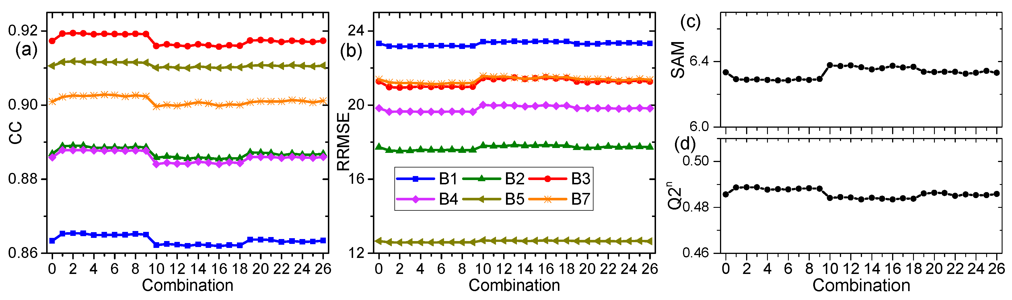
According to Waldo Tobler’s first law of geography [43], reflectance of same land cover type in a small region can change similarly over time, e.g., the maize in adjacent crop fields may grow in similar ways and have analogous spectral features. Therefore, it is reasonable to assume ${\mathsf{\Delta }\mathbf{E}}_C[m,\ast ]$ is same in a sliding-window of coarse-resolution image. With half of the sliding-window size $w_h$, which is measured by the number of coarse pixels and should be defined by user, a sliding-window centred at pixel $[i_c,j_c]$ is selected by $[(i_c-w_h)$:$(i_c+w_h),(j_c-w_h)$:$(j_c+w_h)]$. Size of sliding-window is $w=2\times w_h+1$. Then, $w^2$ linear equations similar with Equation (6) are established with the coarse pixels. To derive ${\mathsf{\Delta }\mathbf{E}}_C[\ast ,b]$ by solving the linear equations, $w^2$ should be greater than $n_m$ [6]. Given the reflectance change is also related to environmental factors (e.g., altitude, morphology, soil type, and fertilization) [40], the assumption that ${\mathsf{\Delta }\mathbf{E}}_C[m,\ast ]$ is the same may be valid only in a small region. Therefore, the definition of $w_h$ should take spatial resolution of the coarse-resolution image and heterogeneity of land surface into consideration. $w_h$ should not be too large, otherwise, it may induce errors in the calculation of ${\mathsf{\Delta }\mathbf{E}}_C[m,\ast ]$.

Theoretically, reflectance of endmembers on Landsat and coarse-resolution images should also be the same. However, sensor difference, caused by differences between fine- and coarse-resolution sensor systems such as bandwidth, solar-viewing geometry conditions, atmospheric correction, and surface reflectance anisotropy [44,45] may exist. The computation of ${\mathsf{\Delta }\mathbf{E}}_C$ is based on $\mathsf{\Delta }\mathbf{C}$. Thus, it has spectral characteristics of coarse-resolution imaging system. To obtain ${\mathsf{\Delta }\mathbf{E}}_F$, sensor difference should be adjusted. Linear and nonlinear models have been proposed to normalize the difference between images of different sensors [46]. Similar to previous studies [47,48], a simple linear model is applied to adjust sensor difference.

$${\mathbf{E}}_F^T[\ast ,b]=a_l\left[b\right]\times {\mathbf{E}}_C^T[\ast ,b]+b_l\left[b\right],\mathrm{with}T=B\mathrm{or}P$$

(10)

In Equation (10), $a_l\left[b\right]$ and $b_l\left[b\right]$ are slope and interception of the linear model for band b and can be calculated by linear regression between the observed fine- and coarse-resolution images. Sensor difference between ${\mathsf{\Delta }\mathbf{E}}_F$ and ${\mathsf{\Delta }\mathbf{E}}_C$ can be adjusted by Equation (11). The $b_l\left[b\right]$ in Equation (10) is reduced after subtraction.

$${\mathsf{\Delta }\mathbf{E}}_F[\ast ,b]=a_l\left[b\right]\times {\mathsf{\Delta }\mathbf{E}}_C[\ast ,b]$$

(11)

In STRUM, ${\mathsf{\Delta }\mathbf{E}}_F$ is directly assigned to fine pixels with same class type according to a fine class image [26]. However, ${\mathsf{\Delta }\mathbf{E}}_F$ is linearly mixed with ${\mathbf{A}}_F^B$ in ISTRUM. Since ${\mathsf{\Delta }\mathbf{E}}_F$ is the local reflectance change of the endmembers, the mixture is only performed on fine pixels that fall in the central coarse pixel. The $\mathsf{\Delta }\mathbf{F}$ is calculated as follow:

$$\mathsf{\Delta }\mathbf{F}[k_{ic},k_{jc},b]=\sum _{m=1}^{n_m}{{\mathbf{A}}_F^B[k_{ic},k_{jc},m]\times \mathsf{\Delta }\mathbf{E}}_F[m,b]$$

(12)

Based on one L-C pair, the Landsat-like image on $T_P$ is finally calculated by

$${\mathbf{F}}^{P\_B}={\mathbf{F}}^B+\mathsf{\Delta }\mathbf{F}$$

(13)

The aforesaid steps describe the prediction model with one L-C pair. When multiple L-C pairs are applied, ${\mathbf{F}}^{P\_B}$ could be first predicted based on each L-C pair and then combined to make a final prediction.

2.4. Implementation of ISTRUM

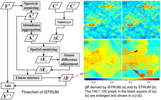
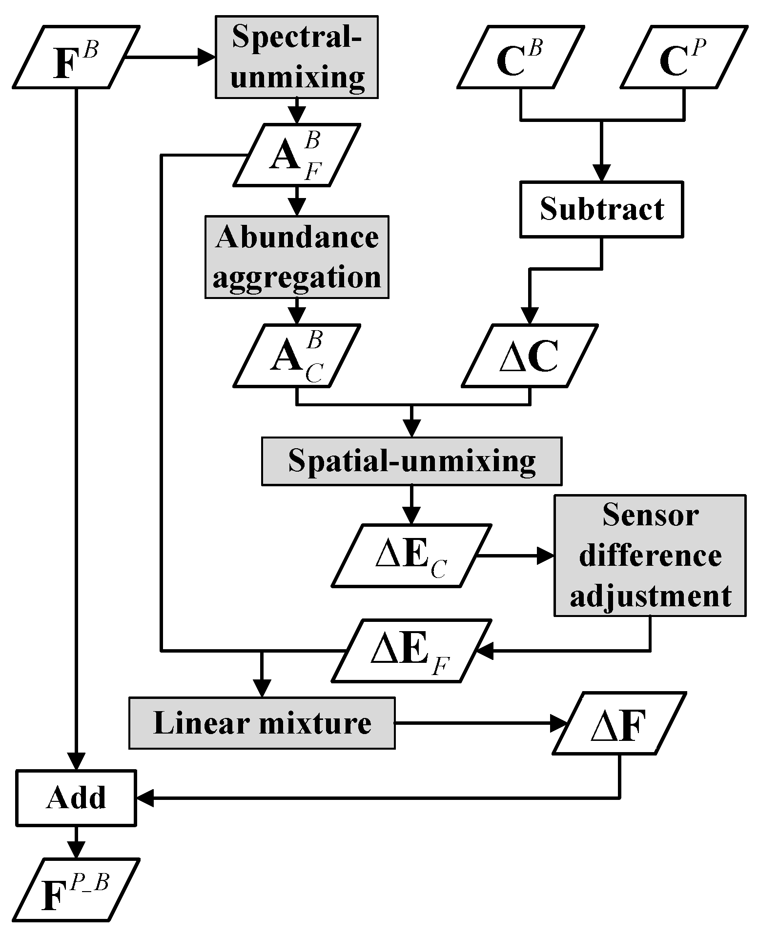
The workflow of ISTRUM is outlined by the flowchart in Figure 1. Key steps (steps with gray background) include spectral-unmixing, abundance aggregation, spatial-unmixing, sensor difference adjustment and linear mixture. Spectral-unmixing is the first step aiming to derive fine-resolution abundance image ${\mathbf{A}}_F^B$ which is used in abundance aggregation and linear mixture. Based on ${\mathbf{A}}_F^B$, coarse-resolution abundance ${\mathbf{A}}_C^B$ is calculated in abundance aggregation. With known ${\mathbf{A}}_C^B$ and coarse-resolution temporal change image $\mathsf{\Delta }\mathbf{C}$, reflectance change of endmembers are calculated in spatial-unmixing process. Derived ${\mathsf{\Delta }\mathbf{E}}_C$ has spectral characteristics of coarse-resolution imaging system. Sensor difference is adjusted to obtain ${\mathsf{\Delta }\mathbf{E}}_F$, which is further linear mixed with ${\mathbf{A}}_F^B$ to obtain fine-resolution temporal change image. Detailed descriptions are in the following subsections.

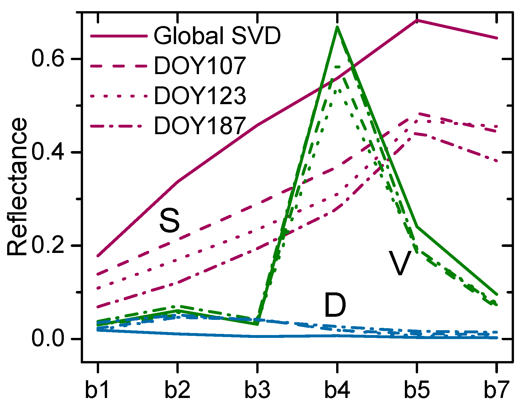
2.4.1. Spectral-Unmixing

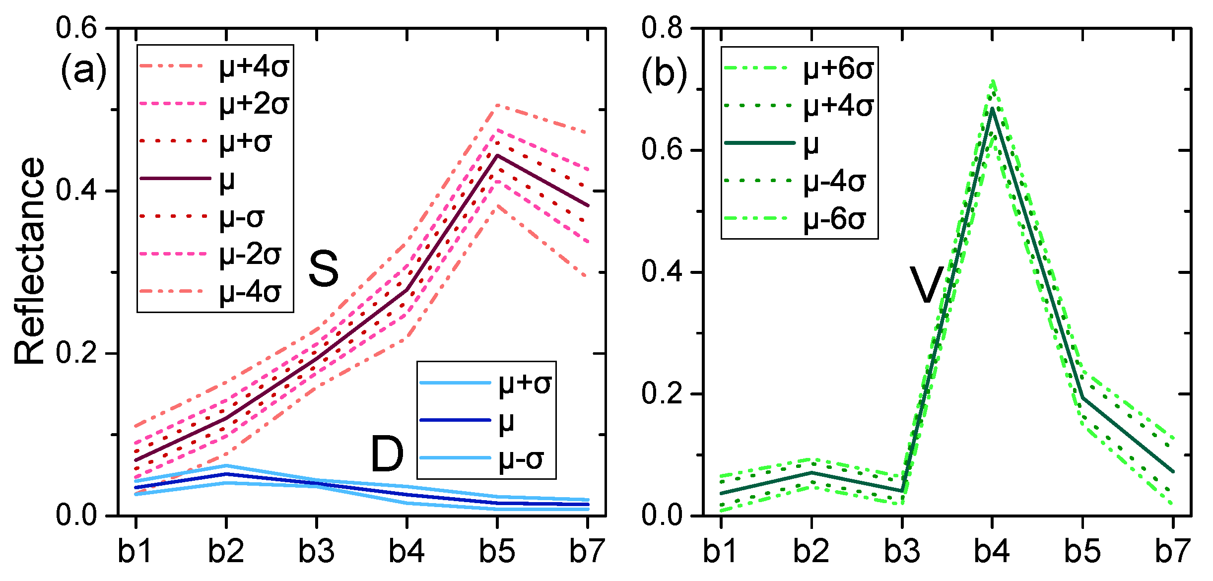
Spectral-unmixing is the first step applied to ${\mathbf{F}}^B$ to obtain ${\mathbf{A}}_F^B$ which is further used to calculate ${\mathbf{A}}_C^B$. To strengthen the applicability of ISTRUM on the global scale, a globally representative spectral linear mixture model (SVD model) for Landsat TM/ETM+/OLI images [39,49,50] was selected in the implementation of spectral-unmixing. Endmembers were classified to three types: substrate (S), vegetation (V), and dark surface (D).

Spectra of endmembers (i.e., ${\mathbf{E}}_F^B$) are extracted from ${\mathbf{F}}^B$ with the approach described by Small [39]. The approach first applies Principal Component Analysis (PCA) to ${\mathbf{F}}^B$, and then selects pure pixels by analyzing the mixing space of the first three primary components. The approach generally selects a suite of pure pixels for each endmember and mean spectra are used in spectral-unmixing. Based on the mixture model, the Fully Constrained Least Square (FCLS) method [51] is used to unmix ${\mathbf{F}}^B$ in the spectral-unmixing process. The computed abundance ${\mathbf{A}}_F^B$ varied from 0 to 1 and the sum of ${\mathbf{A}}_F^B[i_f,j_f,\ast ]$ is 1.

2.4.2. Abundance Aggregation

${\mathbf{A}}_C^B$ is calculated with ${\mathbf{A}}_F^B$ in this process. For a coarse pixel at location $[i_c,j_c]$, abundance of each endmember is calculated by Equation (9). If an endmember abundance is low in a coarse pixel, its errors in spatial-unmixing may be large [6]. Therefore, if the abundance of endmember m is $0<{\mathbf{A}}_C^B[i_c,j_c,m]<t{h}_A$, it is merged to its spectrally most similar class whose abundance should also be greater than 0. In the implementation of ISTRUM, similarity between each endmember is measured by Spectral Angle (SA), which is calculated with ${\mathbf{E}}_F^B$. $t{h}_A$ is set to 0.05 according to previous studies [6,52].

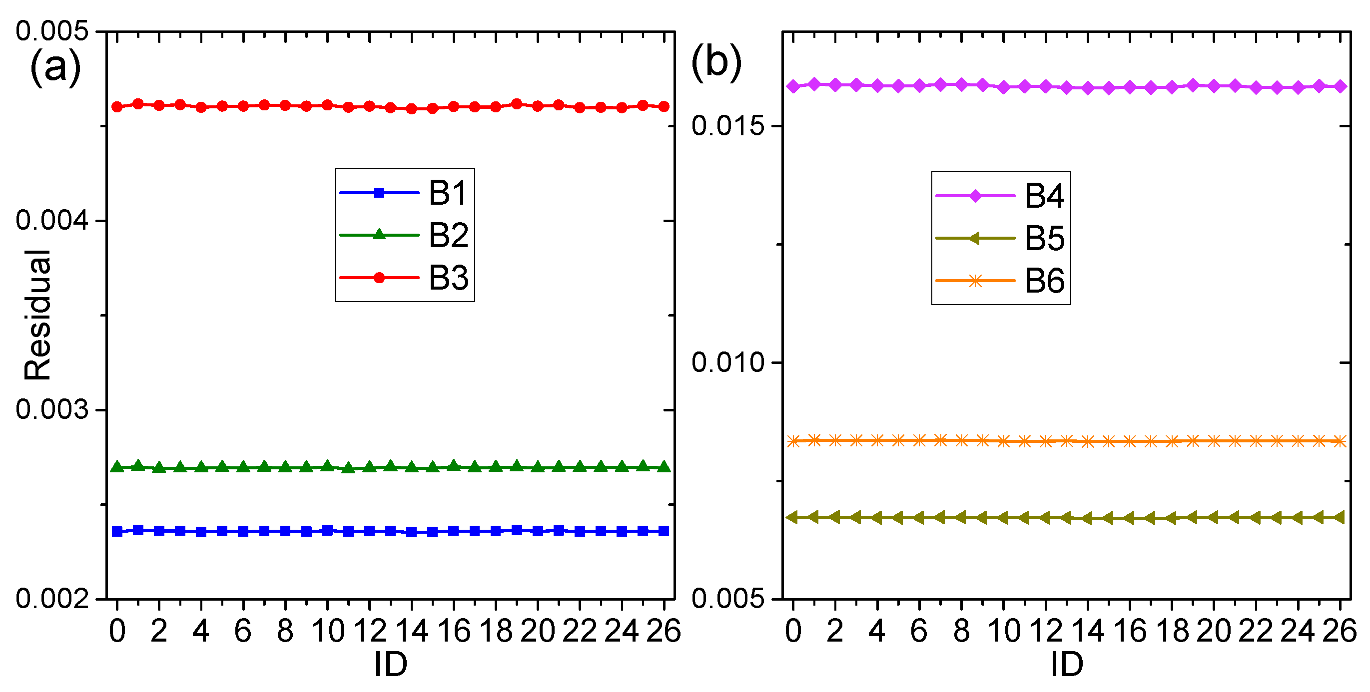
2.4.3. Spatial-Unmixing

The spatial-unmixing process aims to derive $\mathsf{\Delta }{\mathbf{E}}_C$ by solving a system of linear equations. For a coarse pixel at location $[i_c,j_c]$, a sliding-window around it is selected by $[(i_c-w_h)$:$(i_c+w_h),(j_c-w_h)$:$(j_c+w_h)]$ and $w^2$ equations similar with Equation (6) are considered. The least square method is applied to solve the equations because it does not require additional parameters and has been widely implemented in spatial-unmixing based methods [6,25,48]. $\mathsf{\Delta }{\mathbf{E}}_C$ is computed by minimizing Equation (14) based on the Generalized Reduced Gradient Method [53] as follow:

$$\mathsf{\Delta }{\mathbf{E}}_C[\ast ,b]=argmin\left\{\sum _{i=i_c-w_h}^{i_c+w_h}\sum _{j=j_c-w_h}^{j_c+w_h}{\left(\mathsf{\Delta }\mathbf{C}[i,j,b]-\sum _{m=1}^{n_m}{\mathbf{A}}_C^B[i,j,m]\times \mathsf{\Delta }{\mathbf{E}}_C[m,b]\right)}^2\right\}$$

(14)

2.4.4. Sensor Difference Adjustment

Sensor difference is adjusted to obtain $\mathsf{\Delta }{\mathbf{E}}_F$ from $\mathsf{\Delta }{\mathbf{E}}_C$ by means of Equation (11). The coefficient $a_l$ is calculated with ${\mathbf{F}}^B$ and ${\mathbf{C}}^B$. ${\mathbf{F}}^B$ is firstly aggregated to coarse-resolution image ${\mathbf{F}}_a^B$ by averaging the band values of fine pixels that fall in an individual coarse pixel. Then, $a_l\left[b\right]$ is computed by linear regression with ${\mathbf{F}}_a^B[\ast ,\ast ,b]$ as dependent variable and ${\mathbf{F}}^C[\ast ,\ast ,b]$ as independent variable.

2.4.5. Linear Mixture

The $\mathsf{\Delta }{\mathbf{E}}_F$ is linearly mixed with ${\mathbf{A}}_F^B$ (Equation (12)) to reconstruct $\mathsf{\Delta }\mathbf{F}$. The mixture is only applied to fine pixels (i.e., $[k_{ic},k_{jc}]$) falling in the center coarse pixel $[i_c,j_c]$ of the currently selected sliding-window. Because $\mathsf{\Delta }{\mathbf{E}}_F$ represents the reflectance change of endmembers in the sliding-window.

The spatial-unmixing and linear mixture processes are performed pixel-by-pixel for each band of $\mathsf{\Delta }\mathbf{C}$. When all the pixels of $\mathsf{\Delta }\mathbf{C}$ are processed, image $\mathsf{\Delta }\mathbf{F}$ is obtained and the Landsat-like image ${\mathbf{F}}^{P\_B}$ predicted by one L-C pair is finally calculated by Equation (13).

2.4.6. Method to Combine Images Predicted by Multiple L-C Pairs

Suppose there are $n_T$ L-C pairs observed on different base dates $T_B$ with $B\in \{1,2,\dots ,n_T\}$. Each L-C pair could synthesize an individual Landsat-like image ${\mathbf{F}}^{P\_B}$. The final prediction is weighted summation of all the ${\mathbf{F}}^{P\_B}$. Absolute temporal difference ($D_{ijb}^B$) between $T_P$ and $T_B$ is used to calculate the weights. $D_{ijb}^B$ is calculated locally by Equation (15) with $\mathsf{\Delta }\mathbf{C}$ in a sliding-window. The window is same with the one applied in spatial-unmixing because reflectance change of each endmember is assumed to be same in the sliding-window. When $D_{ijb}^B$ value approximates 0, it indicates little reflectance change between $T_B$ and $T_P$, so the prediction based on L-C pair on date $T_B$ should be more reliable. Therefore, ${\mathbf{F}}^{P\_B}$ should have a large weight. Hence, weight $W_{ijb}^B$ is calculated with the reciprocal of $D_{ijb}^B$ in Equation (16). The $W_{ijb}^B$ is for the central coarse pixel $[i_c,j_c]$ of the sliding-window, and fine pixels within it share the same weight. The final prediction (${\mathbf{F}}^{P\_M}$) with multiple L-C pairs is calculated by Equation (17).

$$D_{ijb}^B=\sum _{i=i_c-w_h}^{i_c+w_h}\sum _{j=j_c-w_h}^{j_c+w_h}\left|\mathsf{\Delta }\mathbf{C}\right[i,j,b\left]\right|$$

(15)

$$W_{ijb}^B=\frac{1/D_{ijb}^B}{{\displaystyle \sum _{B=1}^{n_T}}1/D_{ijb}^B}$$

(16)

$${\mathbf{F}}^{P\_M}[k_{ic},k_{jc},b]=\sum _{B=1}^{n_T}{W}_{ijb}^B\times {\mathbf{F}}^{P\_B}[k_{ic},k_{jc},b]$$

(17)

2.5. Differences between ISTRUM and STRUM

Both ISTRUM and STRUM applied spatial-unmixing process directly to the coarse-resolution temporal change image. However, there are some differences. ISTRUM considers the heterogeneity of land surface and regards the pixels on Landsat image are linear mixture of endmembers at the scale of 30 m. Therefore, the fine-resolution abundance image ${\mathbf{A}}_F^B$ is applied in ISTRUM, while class image is used in STRUM. Based on the difference, the $\mathsf{\Delta }{\mathbf{E}}_F$ is further linearly mixed with ${\mathbf{A}}_F^B$ to obtain $\mathsf{\Delta }\mathbf{F}$. The step ensures $\mathsf{\Delta }\mathbf{F}$ to better preserve spectral variability and spatial details than the one derived by STRUM. In addition, sensor difference between $\mathsf{\Delta }{\mathbf{E}}_F$ and $\mathsf{\Delta }{\mathbf{E}}_C$ is considered and adjusted in ISTRUM. While STRUM directly assigns ${\mathbf{E}}_C$ to fine pixels according to the class image without adjusting sensor difference.

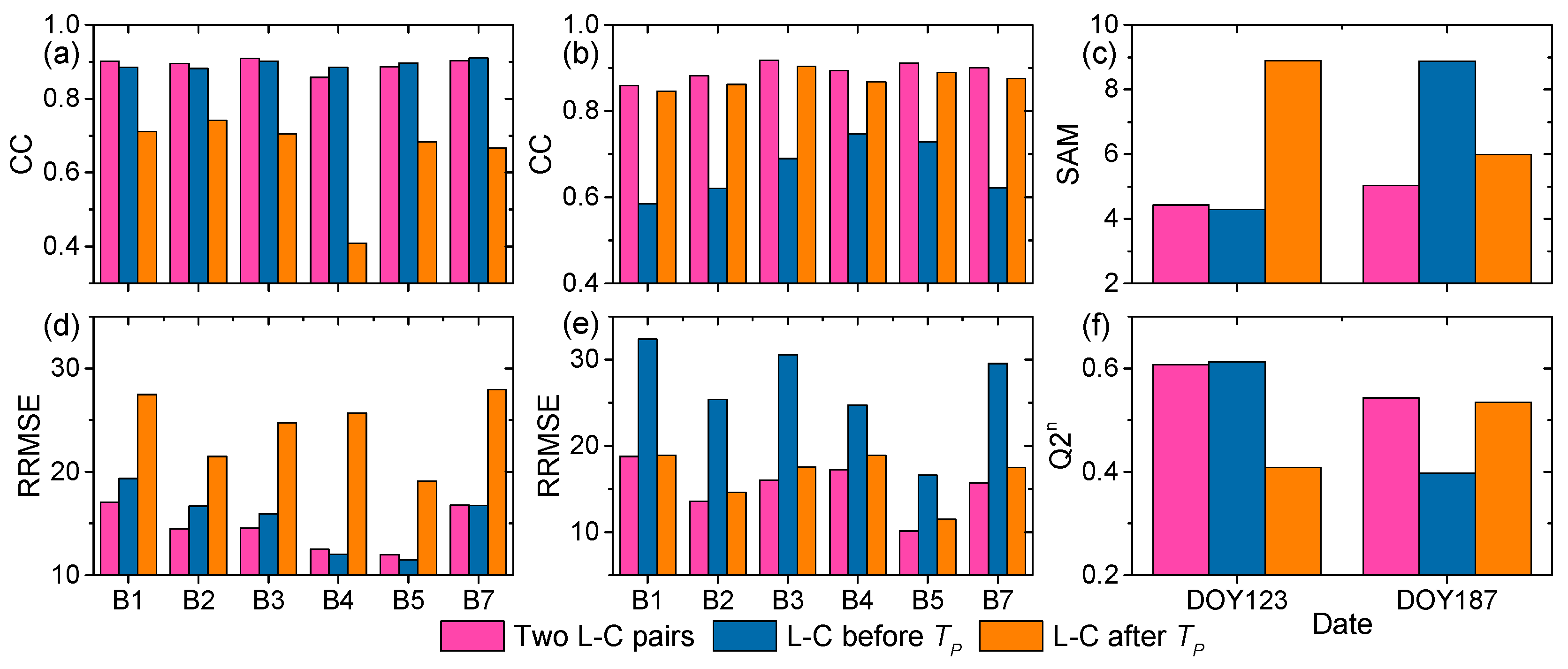
As reference images, the L-C pairs input into the fusion method have significant influence on the prediction accuracy [28,54]. According to [55], two L-C pairs is preferred to be applied in the prediction when temporal change is consistent. ISTRUM can combine prediction results of multiple L-C pairs with a weighted summation method, which strengthens the applicability, while STRUM is applicable with only one L-C pair.

3. Data and Experiment Schemes

3.1. Study Area

Performance of ISTRUM was evaluated with Landsat and MODIS images of Lower Gwydir Catchment (“Gwydir” henceforth) in northern New South Wales (149.2408°E, 29.1146°S), Australia, acquired on 16 April, 2 May, 5 July, and 22 August 2004. Day Of Year (DOY) for each image pair is 107, 123, 187, and 235. The images were shared by Emelyanova et al. [38] and have been widely applied in the evaluation of spatiotemporal image fusion methods [31,38,56]. The images were atmospherically corrected and geographically co-registered [38]. Pixel size of both Landsat and MODIS images was resampled to 25 m with nearest neighbor method by Emelyanova et al. [38]. Because the coarse-resolution image should be in its original spatial resolution to be applied in ISTRUM, we aggregated the MODIS pixel to 500 m resolution. Therefore, spatial resolution ratio S is 20. Dimensions of the Landsat and MODIS images applied in this study are $2000\times 2000\times 6$ and $100\times 100\times 6$, respectively. The Landsat and MODIS images are shown in Figure 2. Temporal dynamics were mainly caused by the vegetation phenology between DOY107 and DOY235. Images on DOY107 and DOY123 are the most similar pairs because of their short time interval. Vegetation growth from DOY187 to DOY235 leads to the reflectance differences in some regions. Bare soil changed to vegetation in large regions from DOY123 to DOY187.

3.2. Experiment Schemes

3.2.1. Comparisons between ISTRUM and STRUM

The experiment aimed to compare the performance of ISTRUM and STRUM. A Landsat-like image was predicted by ISTRUM and STRUM separately based on one L-C pair on its previous date. For example, the Landsat image on DOY123 was predicted by an L-C pair on DOY107 (DOY123by107). There are three experimental combinations: DOY123by107, DOY187by123, and DOY235by187.

In the experiment, ISTRUM and STRUM were tested by setting user defined parameters to different values for all the combinations. Because SVD model is applied in ISTRUM, $n_m$ is 3 and does not need to be defined by user. The parameters required to be defined include $w_h$ and $n_m$ for STRUM and $w_h$ for ISTRUM. $w_h$ was set to $\{1,2,\dots ,10\}$ in step of 1 (i.e., $w\in \{3,5,\dots ,21\}$). $n_m$ was set to 3, 5, 7, and 9 for STRUM. In spectral-unmixing process of ISTRUM, spectra of endmembers were extracted manually with the approach described by Small [39]. To obtain the classification image applied in STRUM, ISODATA was used to classify ${\mathbf{F}}^B$. Observed Landsat images were used to evaluate the prediction accuracy.

Performance of STRUM and ISTRUM under different parameter settings can be compared with results of the experiment. Influence of $w_h$ on ISTRUM could also be analyzed. In addition, performance improvements of ISTRUM were evaluated in detail with DOY187by123 because significant temporal change of vegetation occurred during DOY123 and DOY187.

3.2.2. Sensitivity of ISTRUM to Endmember Variability

The fine-resolution abundance image ${\mathbf{A}}_F^B$ is used to calculate coarse-resolution abundance image which affects the spatial-unmixing process. Derived ${\mathsf{\Delta }\mathbf{E}}_F$ is also linearly mixed with ${\mathbf{A}}_F^B$ to obtain $\mathsf{\Delta }\mathbf{F}$ which directly affects the synthetic image. Therefore, it is necessary to assess whether the uncertainties in ${\mathbf{A}}_F^B$ heavily influence accuracy of ISTRUM.

${\mathbf{A}}_F^B$ is obtained by spectral-unmixing of ${\mathbf{F}}^B$. Endmember variability, caused by the temporal and spatial variability of scene components and imaging conditions [57], is the key factor leading to the uncertainties in ${\mathbf{A}}_F^B$. Assessment of the influence of ${\mathbf{A}}_F^B$ is performed by applying different spectra combinations of endmembers in the spectral-unmixing process. If the accuracy of ISTRUM varies little as the spectra of endmembers varies, it means ISTRUM is robust to endmember variability. Otherwise, ISTRUM is sensitive to endmember variability. Based on this idea, we first determined 27 spectra combinations of endmembers. Each combination was applied to spectral-unmixing process to derive a ${\mathbf{A}}_F^B$. The 27 ${\mathbf{A}}_F^B$ images were separately applied in the prediction of a Landsat-like image with following steps of ISTRUM. Finally, the accuracy of 27 Landsat-like images was calculated and analyzed. Only images on DOY187 and DOY235 were applied in the experiment.

Small and Milesi [49] extracted the spectra of Global SVD endmembers from 100 diverse Landsat TM/ETM+ sub-scenes which were collected globally, and shared the spectra online at http://www.ldeo.columbia.edu/%7esmall/GlobalLandsat/. Although the spectra of endmembers of a specific study area may be different from the Global SVD spectra, we also tested the applicability of Global SVD spectra in experimental combinations DOY123by107, DOY187by123, and DOY235by187. The Global SVD was applied to derive ${\mathbf{A}}_F^B$ in spectral-unmixing process for the prediction of Landsat-like images. Prediction accuracy was compared with results when spectra of endmembers were extracted manually. If the ISTRUM were robust to spectral variability, the Global SVD would be valuable in future application of ISTRUM and only $w_h$ should be defined by user.

3.2.3. ISTRUM with two L-C Pairs

To test ISTRUM with two L-C pairs, Landsat-like images on DOY123 and DOY187 were predicted with L-C pairs on DOY107 and DOY235 (i.e., experimental combinations DOY123by107&235 and DOY187by107&235). The accuracy was compared with results when one L-C pair was applied.

3.2.4. Comparisons between ISTRUM and Benchmark Spatiotemporal Fusion Methods

Performance of ISTRUM was also evaluated by comparing it with benchmark spatiotemporal fusion methods. STDFA, ESTARFM, HCM and FSDAF methods were selected in the comparison. The methods used include spatial-unmixing based, weight-function based, learning based and hybrid methods. STDFA is a spatial-unmixing based method proposed by Wu et al. [25]. It first performs spatial-unmixing process to coarse-resolution image on $T_B$ and $T_P$ separately. Then, it synthesizes fine-resolution image on $T_P$ with a Surface Reflectance Calculation Model (SRCM) [25]. ESTARFM is a weight-function based method and is improved based on STARFM [7]. Since comparison between STRUM and STARFM has been performed in [26], we compared the ISTRUM and ESTARFM in this study because they are both improved methods. In the implementation of ESTARFM, class image was used to identify similar pixels according to [58]. HCM is a learning based method [34,35]. It synthesizes Landsat-like image by applying transformation matrix, which is learned from coarse-resolution images observed on $T_B$ and $T_P$, to Landsat image observed on $T_B$. HCM is a newly developed method and has high performance and computational efficiency [34]. FSDAF is a hybrid method [10]. It considers temporal and spatial variation between $T_B$ and $T_P$, and it has the ability to predict land cover type change.

To synthesize a Landsat-like image, STDFA, HCM and FSDAF require one L-C pair, while ESTARFM requires two L-C pairs, and ISTRUM is applicable with one or more L-C pairs. To ensure the input images are the same for the methods, experimental combinations DOY123by107, DOY187by123, and DOY235by187 were used in the comparison of STDFA, HCM, FSDAF and ISTRUM. Experimental combinations DOY123by107&235 and DOY187by107&235 were used in the comparison of ESTARFM and ISTRUM.

3.3. Quantitative Evaluation Indices

Correlation coefficient (CC), relative root mean square error (RRMSE), spectral angle mapper (SAM), and $Q{2}^n$ [59] between synthetic Landsat-like and observed Landsat image were used to deliver quantitatively assessment of accuracy. The ideal value of CC is 1 and a high value indicates a strong linear relationship between synthetic and observed images. RRMSE is defined as the ratio of the root mean square error of a predicted image to the mean value of the original image and the ratio multiplied by 100 [18]. The ideal value of RRMSE is 0. Low RRMSE indicates small difference in pixel values between synthetic and observed images. Spectral angle with unit of degree between synthesized and observed images was calculated. The ideal value of SAM is 0. Small SAM value indicates high spectral consistency. $Q{2}^n$ is suitable to assess the spatial structure errors for images with an arbitrary number of bands [59]. The ideal value of $Q{2}^n$ is 1. A high $Q{2}^n$ value indicates high spatial consistency between the synthetic image and observed image. Each band of image has a CC and RRMSE value, while each image has a SAM and $Q{2}^n$ value in the assessment.

The reduction in remaining error (RRE) [60] was also used to quantify the improvements in accuracy of different methods. RRE is calculated as

$$RRE=\frac{R{E}_1-R{E}_0}{R{E}_1}\times 100\%$$

(18)

$R{E}_1$ and $R{E}_0$ are remaining errors of the compared methods and ISTRUM, respectively. For CC and $Q{2}^n$, $RE$ is calculated by 1-CC and 1-$Q{2}^n$, respectively. For RRMSE and SAM, $RE$ is the calculated RRMSE and SAM value. The positive RRE means ISTRUM outperformed the compared method while the negative RRE means the compared method had higher accuracy than ISTRUM. The value of RRE indicates the percentage of improvement or degradation of ISTRUM when compared with STRUM, STDFA, ESTARFM and FSDAF.

4. Results

In this section, we present and analyze the experimental results. Section 4.1, Section 4.2, Section 4.3 and Section 4.4 are based on results of experiment described in Section 3.2.1. Section 4.5, Section 4.6 and Section 4.7 are based on results of Section 3.2.2, Section 3.2.3 and Section 3.2.4, respectively.

4.1. Accuracy Comparison of Derived Fine-Resolution Temporal Change Images

Deriving accurate $\mathsf{\Delta }\mathbf{F}$ is the key step for both ISTRUM and STRUM. The derived $\mathsf{\Delta }\mathbf{F}$ of band 4 (B4) in experiment DOY187by123 was used to analyze the improvements of ISTRUM, because B4 is the near infrared (NIR) band which could well indicate the large temporal change from bare soil to vegetation occurred during DOY123 and DOY187. For DOY187by123, when $w_h$ was set to 1 for ISTRUM and STRUM, and $n_m$ was set to 3 for STRUM, both ISTRUM and STRUM had highest accuracy (according to Section 4.3). Therefore, the predicted Landsat-like images with the parameter settings were used in the analysis.

The $\mathsf{\Delta }\mathbf{F}$ of B4 derived in ISTRUM and STRUM were shown in Figure 3. The $\mathsf{\Delta }\mathbf{F}$ derived in ISTRUM pointed out more spectral variability and spatial details than the one derived in STRUM. Because, in ISTRUM, $\mathsf{\Delta }\mathbf{F}$ is calculated by mixing the spectra of endmembers and the abundance image ${\mathbf{A}}_F^B$ which provides well representation of land surface, the mixture could generate different pixel values for $\mathsf{\Delta }\mathbf{F}$ and reserve the spatial characteristics of ${\mathbf{A}}_F^B$, therefore, spectral variability and spatial details are well presented on $\mathsf{\Delta }\mathbf{F}$. However, $\mathsf{\Delta }\mathbf{F}$ is obtained by directly assigning spectra of endmembers to a hard-classification image in STRUM. Therefore, $\mathsf{\Delta }\mathbf{F}$ derived in STRUM shows block effect because the footprints of MODIS pixels are obvious and fine pixels belong to same class type have identical values. Figure 4 shows the scatter plot of derived $\mathsf{\Delta }\mathbf{F}$ versus actual temporal change of B4. Result of ISTRUM was more correlated with the actual $\mathsf{\Delta }\mathbf{F}$ than STRUM, which indicated the improved accuracy of ISTRUM.

4.2. Accuracy Improvements of Every Step in ISTRUM

The accuracy improvements of ISTRUM over STRUM were analyzed step by step with experiment DOY187by123 (

Table 1. Accuracy improvements of every step in ISTRUM. Improvement-1 denotes the change of accuracy based on STRUM when abundance image is applied. Improvement-2 denotes the change of accuracy based on Improvement-1 when sensor difference is adjusted. Accuracy of ISTRUM equals to accuracy of STRUM adds Improvement-1 and Improvement-2.

		B1	B2	B3	B4	B5	B7	Mean
CC	STRUM	0.5589	0.6283	0.6492	0.6477	0.6735	0.5700	0.6213
	Improvement-1	+0.0384	+0.0249	+0.0497	+0.1066	+0.0458	+0.0587	+0.0540
	Improvement-2	+0.0686	+0.0321	+0.0437	+0.0040	+0.0268	+0.0234	+0.0331
	ISTRUM	0.6658	0.6853	0.7425	0.7583	0.7461	0.6521	0.7084
	Overall	+0.1070	+0.0570	+0.0934	+0.1106	+0.0726	+0.0821	+0.0871
	RRE (%)	24.25	15.33	26.61	31.40	22.24	19.09	23.15
	STRUM	31.1155	24.4656	32.5806	29.9281	18.3441	32.9287	28.2271
	Improvement-1	−2.2637	−1.4984	−3.0815	−5.6265	−1.8112	−3.6469	−2.9880
RRMSE	Improvement-2	+1.6177	−1.3239	−1.9427	−0.1755	−0.7202	−0.7985	−0.5572
(%)	ISTRUM	30.4694	21.6433	27.5564	24.1260	15.8128	28.4833	24.6819
	Overall	−0.6460	−2.8223	−5.0241	−5.8020	−2.5313	−4.4453	−3.5452
	RRE (%)	2.08	11.54	15.42	19.39	13.80	13.50	12.62

). Abundance image rather than classification image was applied in ISTRUM, and this improvement was denoted as Improvement-1. Based on Improvement-1, the average increase of CC was about 0.0540 and the average decrease of RRMSE was about 2.99%. The SAM decreased 1.022 and the $Q{2}^n$ increased 0.049. Sensor difference was also considered in ISTRUM. The sensor difference adjustment (Improvement-2) increased CC about 0.0331 while decreased the RRMSE about 0.56%. The SAM decreased 0.134 and the $Q{2}^n$ increased 0.005 after sensor difference adjustment. According to RRE, the average accuracy improvement of ISTRUM is 23.15% in terms of CC and 12.62% of RRMSE.

Among all the bands (i.e., B1–B5 and B7), improvement of B4 is biggest for both CC and RRMSE values. Land surface changed from bare soil to vegetation between DOY123 and DOY187. The growth of vegetation resulted in large reflectance change of B4. Even though pixels in different regions belong to the same vegetation type, their reflectance change is different according to Figure 2. Deriving accurate $\mathsf{\Delta }\mathbf{F}$ of B4 that takes intra-class spectral variability into account will better improve the accuracy. ISTRUM is capable to derive $\mathsf{\Delta }\mathbf{F}$ with spectral variability and spatial details. Therefore, it generated biggest improvement in B4.

4.3. Accuracy ISTRUM and STRUM with Different User Defined Parameters

The user defined parameters $n_m$ and $w_h$ could influence the accuracy of synthetic images [26]. We first compared the performance of ISTRUM and STRUM with the experiments of DOY123by107, DOY187by123 and DOY235by187. $n_m$ was set to 3, 5, 7, and 9 for STRUM and $w_h$ was set to 2. The result (Figure 5) indicates ISTRUM always outperformed STRUM. The accuracy of STRUM decreased as $n_m$ increased. The conclusion was also drawn by Gevaert and García-Haro [26] because the number of unknowns in spatial-unmixing increases when $n_m$ is large. The result implies SVD model is suitable to integrate into ISTRUM because it has three endmembers ($n_m=3$).

To assess the influence of sliding-window size, $w_h$ was set to $\{1,2,\dots ,10\}$ (i.e., $w\in \{3,5,\dots ,21\}$) and performance of ISTRUM and STRUM was compared. $n_m$ of STRUM was set to 3 in the experiment. As w increased, accuracy of both ISTRUM and STRUM decreased (Figure 6). w determines the number of equations to be solved in the spatial-unmixing process. A large w could induce uncertainties in calculation of $\mathsf{\Delta }{\mathbf{E}}_C$ because there are many equations in the computation. In addition, large w means reflectance change of same endmember should be same in a large region. The assumption may be violated because the reflectance change can be spatially varied. Hence, it could induce errors in solving $\mathsf{\Delta }{\mathbf{E}}_C$. Optimal w can be determined with methods proposed in [48]. The optimal $w_h$ is 2 for DOY123by107 and 1 for DOY187by123 and DOY235by187 in the study area. $w_h$ was set to 1 in the following experiments for convenience. The result also revealed ISTRUM outperforms STRUM nearly for every band and sliding-window size. Because based on the improvements which include the utilization of abundance image and the adjustment of sensor difference, ISTRUM could derive more accurate $\mathsf{\Delta }\mathbf{F}$ than STRUM.

4.4. Influence of Base L-C Image Pair on ISTRUM

ISTRUM synthesizes Landsat-like image ${\mathbf{F}}^{P\_B}$ by adding $\mathsf{\Delta }\mathbf{F}$ to ${\mathbf{F}}^B$ (Equation (13)). Accuracy of ${\mathbf{F}}^{P\_B}$ is influenced by the selected base Landsat image ${\mathbf{F}}^B$ and the derived $\mathsf{\Delta }\mathbf{F}$. Once the input L-C image pair is selected in the prediction, ${\mathbf{F}}^B$ is determined. We denote the CC between ${\mathbf{F}}^B$ and ${\mathbf{F}}^P$ as inherent CC (ICC). We also denote the CC between ${\mathbf{F}}^P$ and ${\mathbf{F}}^{P\_B}$, which is a metric of the accuracy of ${\mathbf{F}}^{P\_B}$, as predicted CC (PCC). High ICC can help to generate high PCC to some degree. To analyze influence of base L-C image pair, ICC was calculated and shown in

Table 2. ICC, CCC and PCC of experiment combinations DOY123by107, DOY123by107 and DOY235by187.

	DOY123by107			DOY187by123			DOY235by187
	ICC	CCC	PCC	ICC	CCC	PCC	ICC	CCC	PCC
B1	0.8563	0.8029	0.8796	0.2244	0.0647	0.6658	0.7686	0.7937	0.8633
B2	0.8350	0.7678	0.8772	0.4097	0.4212	0.6853	0.7862	0.7111	0.8868
B3	0.8621	0.8106	0.8968	0.1791	0.0886	0.7425	0.8422	0.8125	0.9172
B4	0.8211	0.7916	0.8830	−0.1429	−0.2370	0.7583	0.6592	0.6380	0.8857
B5	0.8632	0.7647	0.8927	0.3662	0.2403	0.7461	0.8387	0.8439	0.9105
B7	0.8944	0.8206	0.9063	0.0933	−0.0754	0.6521	0.7833	0.7628	0.9009
Mean	0.8554	0.7930	0.8893	0.1883	0.0837	0.7084	0.7797	0.7603	0.8941

. In addition, CC between ${\mathbf{C}}^B$ and ${\mathbf{C}}^P$ was also calculated and denoted as CC of coarse-resolution images (CCC).

Accuracy of DOY123by107 and DOY235by187 were much higher than DOY187by123, which might be partially attributed to their high ICC values. The result also indicated that if the L-C pair with high ICC is available, the user should select it in the application of ISTRUM. However, ${\mathbf{F}}^P$ is not observed in actual application and ICC cannot be calculated in advance. Since CCC has similar trends with ICC, it could be computed in advance and guide the selection of L-C pair in the application.

For DOY187by123, land cover changed from bare soil to vegetation in large regions between DOY123 and DOY187. It caused the low ICC and violated the assumption of ISTRUM that abundance image should be same between $T_B$ and $T_P$. However, PCC is much higher than ICC which indicates the derived $\mathsf{\Delta }\mathbf{F}$ in ISTRUM contributed a lot to the prediction of the Landsat-like image. Although the overall accuracy of synthesized Landsat-like image is not high in DOY187by123, the results implied ISTRUM does not heavily rely on the assumption that abundance image should be same between $T_B$ and $T_P$, and is capable to capture temporal change when the land cover type changed.

4.5. Influence of Endmember Variability on ISTRUM

4.5.1. Sensitivity of ISTRUM to the Endmember Variability

The variation in endmembers’ spectra results in uncertainty of the estimated ${\mathbf{A}}_F^B$ in spectral-unmixing which may further affect the accuracy of ISTRUM. To analyze the sensitivity of ISTRUM to the endmember variability, Landsat image on DOY187 was unmixed with different spectra combinations of SVD, and estimated abundance images were applied to synthesize Landsat-like image on DOY235. Since the approach to extract endmembers selects a suite of pure pixels for S, V, and D, the mean and standard deviation values (denoted as $\mu$ and $\sigma$) of the pixels were used to represent the range of endmember variability.

Considering the $\mu$ and $\sigma$ values of SVD spectra (Figure 7) extracted from Landsat image on DOY187, $\{{\mathrm{S}}_{\mu -4\sigma },{\mathrm{S}}_{\mu },{\mathrm{S}}_{\mu +4\sigma }\}$, $\{{\mathrm{V}}_{\mu -6\sigma },{\mathrm{V}}_{\mu },{\mathrm{V}}_{\mu +6\sigma }\}$, and $\{{\mathrm{D}}_{\mu -\sigma },{\mathrm{D}}_{\mu },{\mathrm{D}}_{\mu +\sigma }\}$ were used to represent the variability of SVD. There were totally 27 ($3\times 3\times 3$) spectra combinations of SVD (

Table 3. The ID of each SVD spectra combination.

ID	S	V	D	ID	S	V	D	ID	S	V	D
0	03S${}_{\mu }$	V${}_{\mu }$	D${}_{\mu }$	9	S${}_{\mu +4\sigma }$	V${}_{\mu }$	D${}_{\mu }$	18	S${}_{\mu -4\sigma }$	V${}_{\mu }$	D${}_{\mu }$
1	S${}_{\mu +4\sigma }$	V${}_{\mu +6\sigma }$	D${}_{\mu +\sigma }$	10	S${}_{\mu -4\sigma }$	V${}_{\mu +6\sigma }$	D${}_{\mu +\sigma }$	19	S${}_{\mu }$	V${}_{\mu +6\sigma }$	D${}_{\mu +\sigma }$
2	S${}_{\mu +4\sigma }$	V${}_{\mu +6\sigma }$	D${}_{\mu -\sigma }$	11	S${}_{\mu -4\sigma }$	V${}_{\mu +6\sigma }$	D${}_{\mu -\sigma }$	20	S${}_{\mu }$	V${}_{\mu +6\sigma }$	D${}_{\mu -\sigma }$
3	S${}_{\mu +4\sigma }$	V${}_{\mu +6\sigma }$	D${}_{\mu }$	12	S${}_{\mu -4\sigma }$	V${}_{\mu +6\sigma }$	D${}_{\mu }$	21	S${}_{\mu }$	V${}_{\mu +6\sigma }$	D${}_{\mu }$
4	S${}_{\mu +4\sigma }$	V${}_{\mu -6\sigma }$	D${}_{\mu +\sigma }$	13	S${}_{\mu -4\sigma }$	V${}_{\mu -6\sigma }$	D${}_{\mu +\sigma }$	22	S${}_{\mu }$	V${}_{\mu -6\sigma }$	D${}_{\mu +\sigma }$
5	S${}_{\mu +4\sigma }$	V${}_{\mu -6\sigma }$	D${}_{\mu -\sigma }$	14	S${}_{\mu -4\sigma }$	V${}_{\mu -6\sigma }$	D${}_{\mu -\sigma }$	23	S${}_{\mu }$	V${}_{\mu -6\sigma }$	D${}_{\mu -\sigma }$
6	S${}_{\mu +4\sigma }$	V${}_{\mu -6\sigma }$	D${}_{\mu }$	15	S${}_{\mu -4\sigma }$	V${}_{\mu -6\sigma }$	D${}_{\mu }$	24	S${}_{\mu }$	V${}_{\mu -6\sigma }$	D${}_{\mu }$
7	S${}_{\mu +4\sigma }$	V${}_{\mu }$	D${}_{\mu +\sigma }$	16	S${}_{\mu -4\sigma }$	V${}_{\mu }$	D${}_{\mu +\sigma }$	25	S${}_{\mu }$	V${}_{\mu }$	D${}_{\mu +\sigma }$
8	S${}_{\mu +4\sigma }$	V${}_{\mu }$	D${}_{\mu -\sigma }$	17	S${}_{\mu -4\sigma }$	V${}_{\mu }$	D${}_{\mu -\sigma }$	26	S${}_{\mu }$	V${}_{\mu }$	D${}_{\mu -\sigma }$

). Landsat image on DOY187 was unmixed by each combination. Absolute differences between abundance images unmixed by ID 1∼26 and ID 0 were calculated and summarized in Figure 8. Variation of endmember spectra leads to obvious changes of abundance especially for S and D. The maximum absolute abundance change is 0.1883 for S and 0.1922 for D with spectra combination ID 14. Even though the variation of spectral is $6\sigma$ for V, the relative variation is small and the maximum absolute abundance change is 0.0765 for V with spectra combination ID 10.

Each abundance image was separately applied in the following steps of ISTRUM and a total of 27 Landsat-like images on DOY257 were synthesized. Accuracy of each image was calculated and shown in Figure 9. It can be seen that variations of CC, RRMSE, SAM and $Q{2}^n$ are small, even though endmember variability resulted in large variation of the abundance images. Maximum (max) and minimum (min) values of CC, RRMSE, SAM and $Q{2}^n$ were identified.

Table 4. Dynamic ranges of CC and RRMSE for each band (B1–B5 and B7) of the synthesized Landsat-like images.

		B1	B2	B3	B4	B5	B7	Mean
CC	min	0.8619	0.8854	0.9157	0.8841	0.9099	0.8996	0.8928
	max	0.8654	0.8890	0.9194	0.8879	0.9118	0.9028	0.8961
RRMSE	min	23.1530	17.5253	20.9421	19.6332	12.5850	21.1355	19.1623
(%)	max	23.4393	17.8413	21.4912	20.0087	12.6957	21.5655	19.5070

shows the maximum and minimum values of CC and RRMSE. Average dynamics for CC and RRMSE are 0.0033% and 0.3446%, respectively. Dynamic range is 6.2837–6.3782 for SAM and 0.4834–0.4888 for $Q{2}^n$. The variation of accuracy is small, even though different spectra of endmembers were applied in spectral-unmixing process of ISTRUM. The results indicated ISTRUM was robust to the endmember variability.

The endmember variability in spectral-unmixing leads to the variation of ${\mathbf{A}}_F^B$. Therefore, the aggregated ${\mathbf{A}}_C^B$ also varied. Because ${\mathbf{A}}_C^B$ was directly applied in spatial-unmixing, the derived $\mathsf{\Delta }{\mathbf{E}}_C$ and $\mathsf{\Delta }{\mathbf{E}}_F$ were also varied. However, $\mathsf{\Delta }{\mathbf{E}}_F$ was linear mixed with ${\mathbf{A}}_F^B$, and the uncertainties in $\mathsf{\Delta }{\mathbf{E}}_F$ and ${\mathbf{A}}_F^B$ may be counteracted in the derived $\mathsf{\Delta }\mathbf{F}$, which directly affects the accuracy of synthetic Landsat-like image.

The residual of spatial-umixing in each experiment were also calculated for further analysis. For coarse pixel $[i_c,j_c,b]$, derived $\mathsf{\Delta }{\mathbf{E}}_C[\ast ,b]$ was mixed with ${\mathbf{A}}_C^B[i_c,j_c,\ast ]$. The residual $\mathcal{E}[i_c,j_c,b]$ is the difference between $\mathsf{\Delta }\mathbf{C}[i_c,j_c,b]$ and the mixture value. The mean absolute value of residual barely changed for each spectra combination of SVD (Figure 10), which indicated the mixture of $\mathsf{\Delta }{\mathbf{E}}_C$ and ${\mathbf{A}}_C^B$ changed little. Since ${\mathbf{A}}_C^B$ is aggregated from ${\mathbf{A}}_F^B$, and $\mathsf{\Delta }{\mathbf{E}}_F$ is linearly adjusted based on $\mathsf{\Delta }{\mathbf{E}}_C$. The $\mathsf{\Delta }\mathbf{F}$, which is mixture of $\mathsf{\Delta }{\mathbf{E}}_F$ and ${\mathbf{A}}_F^B$, should also be stable and guaranteed the stability of synthetic Landsat-like image.

4.5.2. Applicability of Global SVD Endmembers

As ISTRUM was not sensitive to the endmember variability, applicability of Global SVD endmembers [49] was tested in this experiment. Landsat image on DOY107, DOY123 and DOY187 were unmixed by the Global SVD, respectively, and Landsat-like images on their following date were synthesized. The accuracy were compared with experiments when endmembers were extracted from the image itself. Figure 11 shows the differences between Global SVD and extracted SVD spectra. Although the spectra were obviously different, the accuracy varied little and even was improved when Global SVD (

Table 5. Accuracy of ISTRUM when manually extracted SVD (SVD1) and Global SVD (SVD2) were applied separately.

		DOY123by107		DOY187by123		DOY235by187
		SVD1	SVD2	SVD1	SVD2	SVD1	SVD2
	B1	0.8796	0.8850	0.6658	0.6647	0.8633	0.8692
	B2	0.8772	0.8821	0.6853	0.6828	0.8868	0.8943
	B3	0.8968	0.9010	0.7425	0.7369	0.9172	0.9238
CC	B4	0.8830	0.8841	0.7583	0.7460	0.8857	0.8898
	B5	0.8927	0.8963	0.7461	0.7433	0.9105	0.9146
	B7	0.9063	0.9098	0.6521	0.6413	0.9009	0.9054
	Mean	0.8893	0.8930	0.7084	0.7025	0.8941	0.8995
	B1	19.7897	19.3336	30.4694	30.3104	23.3271	22.8452
	B2	16.9933	16.6672	21.6433	21.7683	17.7299	17.0448
	B3	16.2304	15.9122	27.5564	27.7627	21.2792	20.2884
RRMSE (%)	B4	12.1429	12.0233	24.1260	24.6530	19.8399	19.4376
	B5	11.6851	11.4985	15.8128	15.9536	12.6622	12.3848
	B7	17.0202	16.7432	28.4833	28.8972	21.3935	20.7886
	Mean	15.6436	15.3630	24.6819	24.8909	19.3719	18.7983
SAM	-	4.3867	4.2934	8.2561	8.3265	6.3366	6.1858
$Q{2}^n$	-	0.6025	0.6119	0.4145	0.4179	0.4855	0.4947

) was used. The results implied the potential to directly apply Global SVD endmembers in future applications of ISTRUM. Since SVD is a representative spectral mixture model for globally archived Landsat TM/ETM+/OLI images and the Global SVD endmembers are extracted from a global Landsat dataset [39,49,50]. The integration of SVD model strengthens the applicability of ISTRUM for Landsat images observed on a global scale. The direct utilization of the Global SVD endmembers makes ISTRUM friendly to use because only $w_h$ needs to be defined by the users.

4.6. Experiment with Two L-C Pairs

To test ISTRUM with more than one L-C pairs, Landsat-like images on DOY123 and DOY187 were predicted by L-C pairs on DOY107 and DOY235. The Global SVD endmembers were used in the spectral-unmixing and $w_h$ was set to 1. The results are shown in Figure 12. The prediction accuracy was low when there was one L-C pair and significant temporal change occurred between $T_B$ and $T_P$. However, the accuracy was improved when another L-C pair with small temporal change was applied. The accuracy of Landsat-like image which was synthesized by two L-C pairs was higher than the one which was synthesized by either one of two L-C pairs. However, for synthetic image on DOY123 based on two L-C pairs, accuracy of B4, B5, and B7 decreased slightly when compared with the image synthesized by one L-C pair on DOY107. Because the long time interval between DOY123 and DOY235 (112 days) can complicate the temporal change of land surface, which degrades the accuracy of prediction if land cover type have changed.

4.7. Comparisons of ISTRUM, STDFA, ESTARFM, HCM, and FSDAF

ISTRUM was compared with STDFA, ESTARFM, HCM, and FSDAF, which are benchmark spatiotemporal image fusion methods. Performance of different methods was evaluated in terms of quantitative accuracy and computational efficiency.

4.7.1. Quantitative Accuracy Comparison

Table 6. Quantitative assessment of synthesized Landsat-like images by STDFA, HCM, FADAF and ISTRUM. The R in the second parentheses denotes the rank of the method.

			STDFA(RRE %)(R)	HCM(RRE %)(R)	FSDAF(RRE %)(R)	ISTRUM(R)
		B1	0.8660 (14.17) (4)	0.8949 (−9.41) (2)	0.8970 (−11.66) (1)	0.8850 (3)
		B2	0.8556 (18.32) (4)	0.8939 (−11.20) (2)	0.8951 (−12.43) (1)	0.8821 (3)
		B3	0.8710 (23.24) (4)	0.9045 (−3.70) (2)	0.9095 (−9.35) (1)	0.9010 (3)
	CC	B4	0.8424 (26.49) (4)	0.8820 (1.79) (3)	0.8896 (−4.96) (1)	0.8841 (2)
		B5	0.8653 (23.01) (4)	0.9048 (−8.97) (2)	0.9065 (−10.88) (1)	0.8963 (3)
		B7	0.8736 (28.60) (4)	0.9094 (0.41) (3)	0.9102 (−0.51) (1)	0.9098 (2)
DOY123		Mean	0.8623 (22.31) (4)	0.8983 (−5.18) (2)	0.9013 (−8.30) (1)	0.8930 (3)
by107	R	B1	22.5714 (14.34) (4)	18.0438 (−7.15) (1)	19.0042 (−1.73) (2)	19.3336 (3)
		B2	17.9176 (6.98) (4)	15.1464 (−10.04) (2)	14.5512 (−14.54) (1)	16.6672 (3)
		B3	18.2034 (12.59) (4)	15.4631 (−2.90) (2)	14.5452 (−9.40) (1)	15.9122 (3)
	RMSE (%)	B4	14.9230 (19.43) (4)	11.8142 (−1.77) (2)	11.3644 (−5.80) (1)	12.0233 (3)
		B5	13.1452 (12.53) (4)	11.0762 (−3.81) (2)	10.7289 (−7.17) (1)	11.4985 (3)
		B7	19.5603 (14.40) (4)	17.0861 (2.01) (3)	16.6975 (−0.27) (1)	16.7432 (2)
		Mean	17.7202 (13.38) (4)	14.7716 (−3.94) (2)	14.4819 (−6.49) (1)	15.3630 (3)
	SAM	-	5.0768 (15.43) (4)	3.9739 (−8.04) (1)	4.0982 (−4.76) (2)	4.2934 (3)
	$Q{2}^n$	-	0.5633 (11.13) (4)	0.6304 (−5.02) (1)	0.5906 (5.20) (3)	0.6119 (2)
		B1	0.5567 (24.35) (4)	0.6457 (5.36) (3)	0.6061 (14.87) (2)	0.6647 (1)
		B2	0.6287 (14.56) (4)	0.6654 (5.17) (3)	0.6687 (4.23) (2)	0.6828 (1)
		B3	0.6461 (25.66) (4)	0.6946 (13.87) (3)	0.7164 (7.24) (2)	0.7369 (1)
	CC	B4	0.6476 (27.93) (3)	0.5835 (39.03) (4)	0.7671 (−9.07) (1)	0.7460 (2)
		B5	0.6729 (21.54) (4)	0.6917 (16.75) (3)	0.7396 (1.45) (2)	0.7433 (1)
		B7	0.5672 (17.12) (4)	0.6345 (1.84) (3)	0.6431 (−0.51) (1)	0.6413 (2)
DOY187		Mean	0.6199 (21.86) (4)	0.6526 (13.67) (3)	0.6902 (3.04) (2)	0.7025 (1)
by 123		B1	31.2501 (3.01) (3)	31.4319 (3.57) (4)	27.9180 (-8.57) (1)	30.3104 (2)
		B2	24.4620 (11.01) (4)	22.2539 (2.18) (3)	21.4301 (−1.58) (1)	21.7683 (2)
		B3	32.7879 (15.33) (4)	30.3641 (8.57) (3)	28.1812 (1.49) (2)	27.7627 (1)
	RMSE (%)	B4	29.9387 (17.66) (3)	32.2695 (23.60) (4)	23.7693 (−3.72) (1)	24.6530 (2)
		B5	18.4070 (13.33) (4)	18.4039 (13.31) (3)	15.8285 (−0.79) (1)	15.9536 (2)
		B7	33.1154 (12.74) (4)	30.7261 (5.95) (3)	27.9871 (−3.25) (1)	28.8972 (2)
		Mean	28.3268 (12.18) (4)	27.5749 (9.53) (3)	24.1857 (−2.74) (1)	24.8909 (2)
	SAM	-	9.4225 (11.63) (4)	9.2288 (9.78) (3)	8.0472 (−3.47) (1)	8.3265 (2)
	$Q{2}^n$	-	0.3603 (9.00) (4)	0.4212 (−0.58) (1)	0.3613 (8.86) (3)	0.4179 (2)
		B1	0.8409 (17.78) (4)	0.8466 (14.72) (3)	0.8756 (−5.17) (1)	0.8692 (2)
		B2	0.8665 (20.78) (4)	0.8790 (12.60) (3)	0.9003 (−6.03) (1)	0.8943 (2)
		B3	0.8981 (25.23) (4)	0.9033 (21.24) (3)	0.9254 (−2.17) (1)	0.9238 (2)
	CC	B4	0.8482 (27.39) (4)	0.8522 (25.42) (3)	0.8932 (−3.26) (1)	0.8898 (2)
		B5	0.8919 (21.06) (4)	0.9067 (8.49) (3)	0.9215 (−8.72) (1)	0.9146 (2)
		B7	0.8731 (25.50) (4)	0.8949 (9.98) (3)	0.9098 (−4.82) (1)	0.9054 (2)
DOY235		Mean	0.8698 (22.96) (4)	0.8805 (15.41) (3)	0.9043 (−5.03) (1)	0.8995 (2)
by 187		B1	25.0868 (8.94) (4)	24.2451 (5.77) (3)	22.2098 (−2.86) (1)	22.8452 (2)
		B2	19.2244 (11.34) (4)	17.9257 (4.91) (3)	16.4230 (−3.79) (1)	17.0448 (2)
		B3	23.5860 (13.98) (4)	22.7859 (10.96) (3)	19.9418 (−1.74) (1)	20.2884 (2)
	RMSE (%)	B4	22.8159 (14.81) (3)	22.9792 (15.41) (4)	18.6695 (−4.11) (1)	19.4376 (2)
		B5	13.8405 (10.52) (4)	13.0303 (4.95) (3)	11.9447 (−3.68) (1)	12.3848 (2)
		B7	24.3245 (14.54) (4)	22.0212 (5.60) (3)	20.2364 (−2.73) (1)	20.7886 (2)
		Mean	21.4797 (12.35) (4)	20.4979 (7.94) (3)	18.2375 (−3.15) (1)	18.7983 (2)
	SAM	-	6.9054 (10.42) (4)	6.5378 (5.38) (3)	6.0875 (−1.61) (1)	6.1858 (2)
	$Q{2}^n$	-	0.4593 (6.55) (4)	0.4935 (0.24) (2)	0.4807 (2.71) (3)	0.4947 (1)

shows the accuracy of STDFA, HCM, FSDAF and ISTRUM performed with one L-C pair.

It can be seen that ISTRUM always outperformed STDFA which is another spatial-unmixing based method. Average accuracy of ISTRUM is generally 10% higher than STDFA. Classification image is applied in spatial-unmixing process of STDFA, thus, downscaled fine-resolution image lacks spectral variability. In addition, in order to apply the Surface Reflectance Calculation Model (SRCM), STDFA performs spatial-unmixing to coarse-resolution image on $T_B$ and $T_P$ separately [25]. The two spatial-unmixing processes can increase uncertainties and induce errors.

ISTRUM outperformed HCM slightly in DOY187by123 and DOY235by187, while HCM was slightly better in DOY123by107. The transformation matrix learned from coarse-resolution images heavily influences the accuracy of HCM. Time interval is 16 days for DOY123by107 and temporal change is insignificant. The strong correlation between images on DOY123 and DOY187 (Table 2) contributed to deriving a reliable transformation matrix in the learning process. Therefore, HCM had higher accuracy. However, significant temporal change occurred for DOY187by123 and DOY235by187 due to the long time interval. The change degraded the accuracy of transformation matrix in HCM. Thus, ISTRUM outperformed HCM. The result indicates ISTRUM has better performance than HCM when temporal change is significant.

For DOY187by123, CC indicates ISTRUM slightly outperforms FSDAF when we compare the correlation between synthesized and observed image. However, RRMSE indicates the image synthesized by FSDAF has smaller difference with observed image than the one synthesized by ISTRUM. The inconsistency between CC and RRMSE is reasonable because CC measures the strength of linear relationship while RRMSE measures the difference of pixel values between observed and synthetic image. The inconsistence was also found in [34]. The change of land surface leads to the reflectance changing at varied magnitudes for different bands, which means a band-wise difference in the intensity of temporal change. Since performance of different methods is influenced by factors such as the complexity and intensity of temporal change, spatial heterogeneity and optimal parameters [54], the accuracy is band dependent. In general, the results indicate FSDAF has the best performance in most cases. However, it is also worth noting that FSDAF takes advantages of both spatial-unmixing and weigh-function based methods and predicts land cover type change with a spatial interpolation method which is suitable to deal with small land cover type change [10]. Nonetheless, land cover type change is not specifically considered in STDFA, HCM and ISTRUM, which limits their performance when compared with FSDAF.

Among all methods, accuracy of DOY187by123 is lower than DOY123by107 and DOY235by187 because of the weak correlation between images on DOY123 and DOY187. This result indicates selection of L-C image pair is important for all the compared methods. Accuracy could be improved by selecting L-C pair with high correlation [54].

Table 7. Comparison between ESTARFM and ISTRUM.

		DOY123By107&235		DOY187By107&235
		ESTARFM (RRE %)	ISTRUM	ESTARFM (RRE %)	ISTRUM
	B1	0.9099 (−8.98)	0.9018	0.8664 (−5.28)	0.8594
	B2	0.8957 (−0.84)	0.8948	0.8895 (−7.06)	0.8817
	B3	0.9070 (1.81)	0.9087	0.9219 (−4.36)	0.9185
CC	B4	0.8222 (19.78)	0.8574	0.8822 (9.67)	0.8936
	B5	0.8676 (14.17)	0.8864	0.8988 (12.82)	0.9118
	B7	0.8873 (13.75)	0.9028	0.8936 (5.85)	0.8998
	Mean	0.8816 (6.62)	0.8920	0.8921 (1.94)	0.8941
	B1	17.4677 (2.47)	17.0360	17.0265 (−10.44)	18.8046
	B2	14.2008 (−1.94)	14.4764	12.7523 (−6.37)	13.5640
	B3	14.4847 (−0.28)	14.5256	15.5686 (−3.13)	16.0557
RRMSE (%)	B4	14.1695 (11.65)	12.5183	17.6942 (2.41)	17.2672
	B5	12.6173 (5.17)	11.9652	10.6253 (4.65)	10.1311
	B7	17.6448 (4.85)	16.7899	16.1206 (2.64)	15.6947
	Mean	15.0975 (3.65)	14.5519	14.9646 (−1.71)	15.2529
SAM	-	4.8290 (8.19)	4.4335	5.0645 (0.68)	5.0299
$Q{2}^n$	-	0.5984 (2.12)	0.6069	0.5536 (−2.37)	0.5430

summarizes the accuracy of ESTARFM and ISTRUM for experiments with two L-C pairs. ISTRUM outperformed ESTARFM for some bands because the intensity of temporal change is different for each band. The difference in theoretical basis of ISTRUM and ESTARFM results in their abilities to deal with temporal change of different complexity and intensity being varied. In general, performance of ISTRUM and ESTARFM are comparable because the accuracy values are close for both DOY123by107&235 and DOY187by107&235. The maximum difference is 0.0104% for CC and 0.55% for RRMSE.

4.7.2. Computational Efficiency

In this study, ISTRUM was implemented in Interactive Data Language (IDL) development environment. The code can be found at URL: https://github.com/JianhangMa/ISTRUM.git. Experiments were run on a PC with an Intel(R) Core(TM) i5-7300HQ 2.50 GHz CPU and 8 GB memory. Average time for each execution is shown in

Table 8. Execution time for STDFA, ISTRUM, HCM, ESTARFM and FSDAF. s, m, and h denote second, minute, and hour, respectively.

	STDFA	ISTRUM	HCM	ESTARFM	FSDAF
Time	15.387 s	19.025 s	10.25 m	2.54 h	6.22 h

. ISTRUM is about 32 times faster than HCM, 480 times faster than ESTARFM and 1178 times faster than FSDAF. Computational efficiency of ISTRUM is much higher than ESTARFM and FSDAF. For large-scale and long-term applications of spatiotemporal fusion methods, ISTRUM provides a valuable alternative because it can synthesize images with acceptable accuracy in a short time.

5. Discussion

Spatiotemporal image fusion is a feasible and cost-efficient approach to synthesize images with high spatial and temporal resolution [15]. Spatial-unmixing based method is one kind of the most widely studied spatiotemporal fusion methods [6,25,26,40,41]. One challenge is that the image derived in spatial-unmixing based method generally lacks spectral variability and spatial details [10,26,27]. 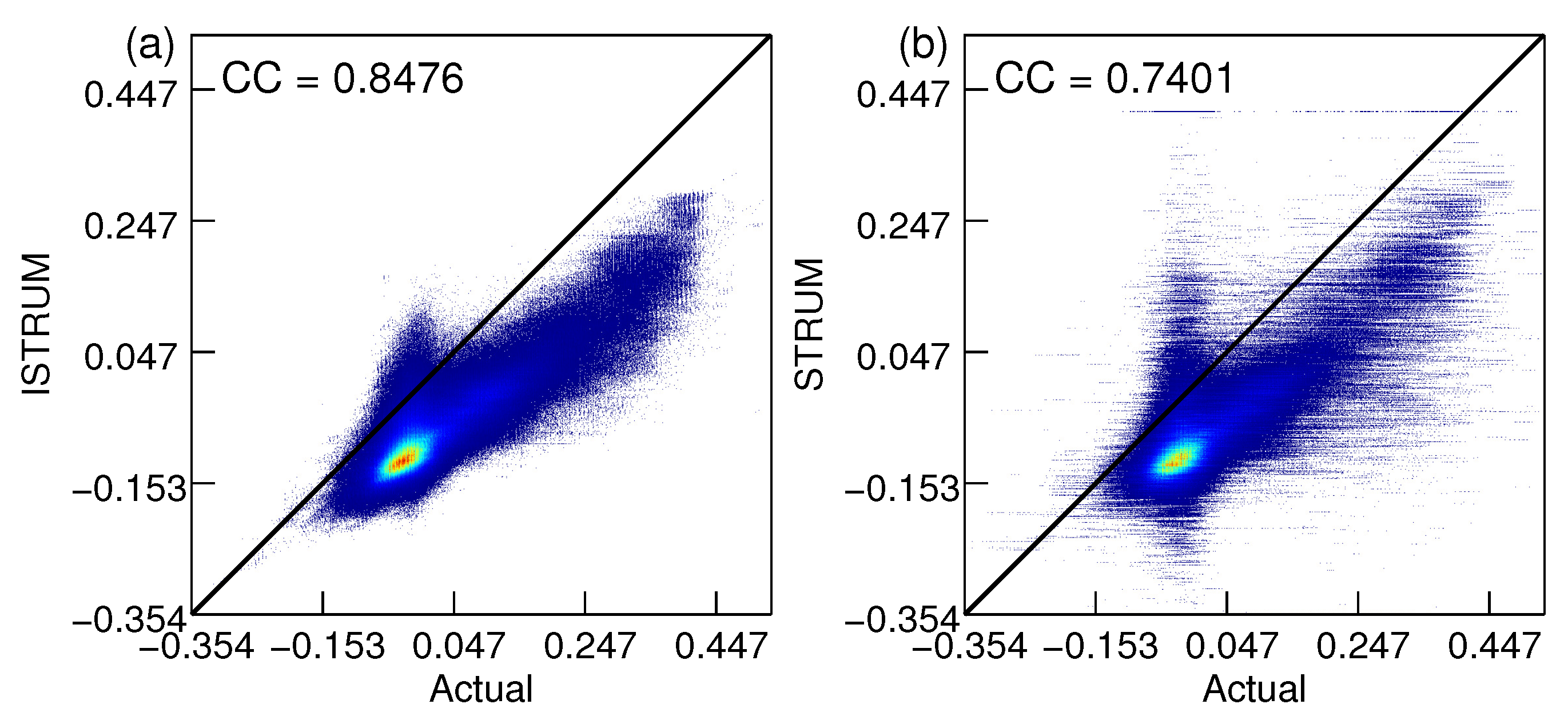To tackle the problem, this study improved the STRUM, which is a well-performing spatial-unmixing based method [26], by applying fine-resolution abundance image. Experimental results revealed ISTRUM generated higher accuracy than STRUM and was competitive with benchmark spatiotemporal fusion methods. Based on the results in this study, relevant issues are discussed in the following paragraphs.

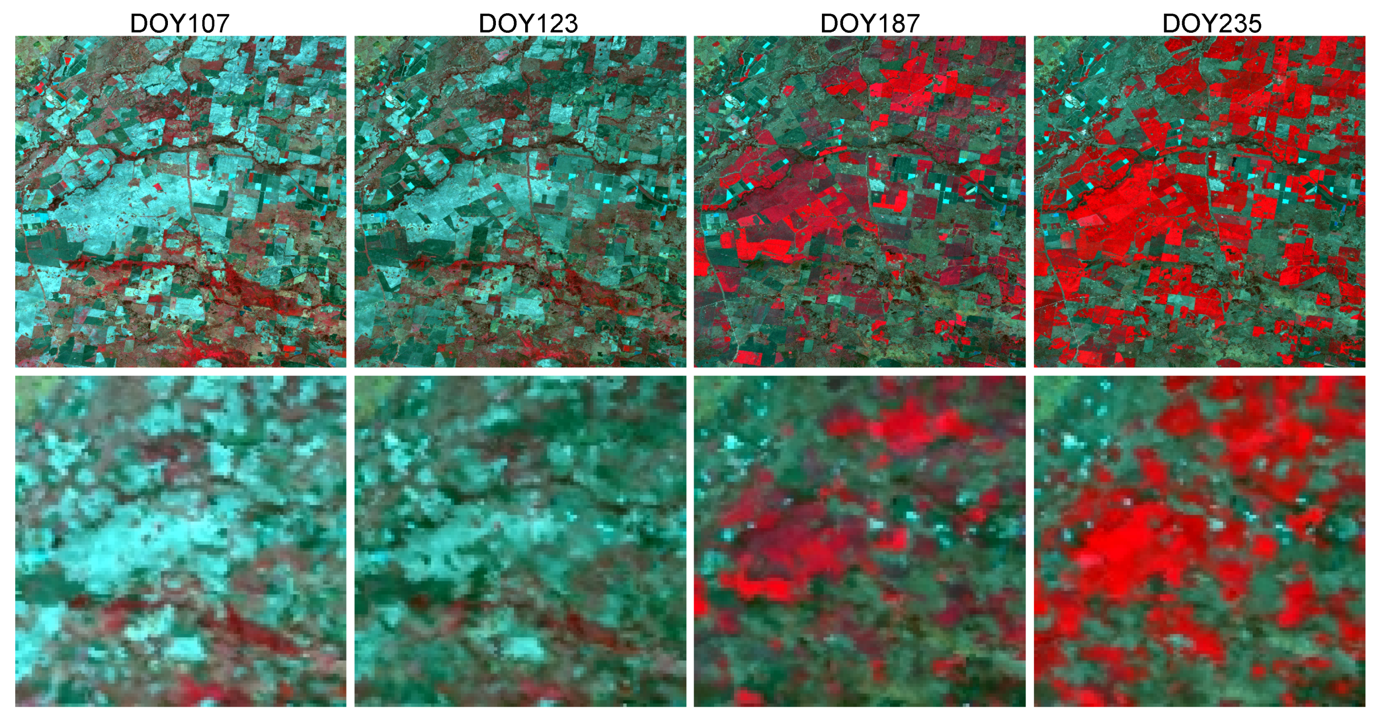
Used as the base images in spatiotemporal fusion methods, L-C image pair is significant to improve the accuracy of synthetic image. Accuracy of the same method varied greatly when input L-C pair is different. In our study, Landsat-like image on DOY187 synthesized based on L-C pair on DOY235 (Section 4.4) has higher accuracy than the one based on DOY123 and DOY107. The accuracy of Landsat-like image is improved when L-C image pair strongly correlates to images on $T_P$. Cheng et al. [28] found accuracy increased as the time interval between $T_B$ and $T_P$ decreased because the likelihood of large temporal change is low and correlation between images on $T_B$ and $T_P$ is high when the time interval is short. According to the correlation between coarse-resolution images on $T_B$ and $T_P$, optimal L-C pair can be determined [54]. In addition, multiple L-C pairs can also improve the accuracy for situations when more than one L-C pair are available.

Since accuracy of spatiotemporal fusion methods is influenced by spatial heterogeneity [5,7], land cover type [48], and the complexity of temporal change [38], performance of the methods varied under different conditions. There is no universal method that performs well under all conditions [34]. For example, although FSDAF considers land cover type change, it has problems in overestimating spatial variations [11]; and ESTARFM improves the accuracy in heterogeneous regions but has problems in estimating nonlinear reflectance changes [38]. Our study also found ISTRUM outperformed HCM when temporal change was large while HCM was better when temporal change was small. Therefore, selecting and combining different methods according to the conditions is meaningful in application [34]. For example, to synthesize time series NDVI, methods with better performance at Red and NIR bands are preferred considering the fusion accuracy is band dependent. In addition, for large area and long term applications of spatiotemporal fusion methods, processing many images is required. The trade-off between accuracy and computational efficiency should be considered. With one user defined parameter and high computational efficiency, ISTRUM provides an easy-to-use and efficient alternative.

Fine- and coarse-resolution images are generally regarded as consistent when developing the spatiotemporal fusion methods [10,11]. However, sensor difference commonly existed and impacts fusion accuracy. Xie et al. [54] found MODIS images with smaller view zenith angle produce better predictions. Preprocessing to reduce of sensor difference helps to improve the accuracy. Models to adjust sensor difference are worth of integration into spatiotemporal fusion methods. Similar with previous studies [47,48], ISTRUM adjusted the sensor difference with a simple linear model and improved the performance to some degree. However, nonlinear models [46] to normalize the inconsistency between fine- and coarse-resolution images are worth studying in the future.

6. Conclusions

To tackle the shortcomings of STRUM, this study proposed ISTRUM to improve STRUM from three aspects: (1) apply fine-resolution abundance image rather than hard-classification image in the spatial-unmixing process; (2) adjust sensor difference between fine- and coarse-resolution images; and (3) strengthen the applicability when multiple L-C image pairs are utilized. Experimental results demonstrated that:

(1)

All three improvements contribute to improving performance of ISTRUM when compared with STRUM. ISTRUM is robust to endmember variability, and the spectra of Global SVD endmembers could be directly applied. Sliding-window size is the only parameter that needs to be defined by the user and decreases the accuracy of ISTRUM when it is large.

(2)

The selection of L-C image pair plays a significant role in the fusion methods. Accuracy is improved when the L-C image pair is strongly correlated with the image on prediction date.

(3)

Performance of the fusion methods are different under different conditions. Selecting and combining different methods according to the conditions is meaningful in application. ISTRUM is an easy-to-use and efficient alternative to synthesize time series of Landsat-like images on a global scale.

References

1. Wulder, M.A.; White, J.C.; Loveland, T.R.; Woodcock, C.E.; Belward, A.S.; Cohen, W.B.; Fosnight, E.A.; Shaw, J.; Masek, J.G.; Roy, D.P. The global Landsat archive: Status, consolidation, and direction. Remote Sens. Environ. 2016, 185, 271–283. [Google Scholar] [CrossRef]
2. Fisher, J.I.; Mustard, J.F.; Vadeboncoeur, M.A. Green leaf phenology at Landsat resolution: Scaling from the field to the satellite. Remote Sens. Environ. 2006, 100, 265–279. [Google Scholar] [CrossRef]
3. Zheng, B.; Myint, S.W.; Thenkabail, P.S.; Aggarwal, R.M. A support vector machine to identify irrigated crop types using time-series Landsat NDVI data. Int. J. Appl. Earth Obs. Geoinf. 2015, 34, 103–112. [Google Scholar] [CrossRef]
4. Kovalskyy, V.; Roy, D. The global availability of Landsat 5 TM and Landsat 7 ETM+ land surface observations and implications for global 30m Landsat data product generation. Remote Sens. Environ. 2013, 130, 280–293. [Google Scholar] [CrossRef]
5. Gao, F.; Masek, J.; Schwaller, M.; Hall, F. On the blending of the Landsat and MODIS surface reflectance: Predicting daily Landsat surface reflectance. IEEE Trans. Geosci. Remote Sens. 2006, 44, 2207–2218. [Google Scholar]
6. Zurita-Milla, R.; Kaiser, G.; Clevers, J.; Schneider, W.; Schaepman, M. Downscaling time series of MERIS full resolution data to monitor vegetation seasonal dynamics. Remote Sens. Environ. 2009, 113, 1874–1885. [Google Scholar] [CrossRef]
7. Zhu, X.; Chen, J.; Gao, F.; Chen, X.; Masek, J.G. An enhanced spatial and temporal adaptive reflectance fusion model for complex heterogeneous regions. Remote Sens. Environ. 2010, 114, 2610–2623. [Google Scholar] [CrossRef]
8. Huang, B.; Song, H. Spatiotemporal Reflectance Fusion via Sparse Representation. IEEE Trans. Geosci. Remote Sens. 2012, 50, 3707–3716. [Google Scholar] [CrossRef]
9. Song, H.; Huang, B. Spatiotemporal Satellite Image Fusion through One-Pair Image Learning. IEEE Trans. Geosci. Remote Sens. 2013, 51, 1883–1896. [Google Scholar] [CrossRef]
10. Zhu, X.; Helmer, E.H.; Gao, F.; Liu, D.; Chen, J.; Lefsky, M.A. A flexible spatiotemporal method for fusing satellite images with different resolutions. Remote Sens. Environ. 2016, 172, 165–177. [Google Scholar] [CrossRef]
11. Wang, Q.; Atkinson, P.M. Spatio-temporal fusion for daily Sentinel-2 images. Remote Sens. Environ. 2018, 204, 31–42. [Google Scholar] [CrossRef]
12. Zhao, Y.; Huang, B.; Song, H. A robust adaptive spatial and temporal image fusion model for complex land surface changes. Remote Sens. Environ. 2018, 208, 42–62. [Google Scholar] [CrossRef]
13. Yue, L.; Shen, H.; Li, J.; Yuan, Q.; Zhang, H.; Zhang, L. Image super-resolution: The techniques, applications, and future. Signal Process. 2016, 128, 389–408. [Google Scholar] [CrossRef]
14. Shen, H.; Meng, X.; Zhang, L. An Integrated Framework for the Spatio-Temporal-Spectral Fusion of Remote Sensing Images. IEEE Trans. Geosci. Remote Sens. 2016, 54, 7135–7148. [Google Scholar] [CrossRef]
15. Zhu, X.; Cai, F.; Tian, J.; Williams, T.K.A. Spatiotemporal Fusion of Multisource Remote Sensing Data: Literature Survey, Taxonomy, Principles, Applications, and Future Directions. Remote Sens. 2018, 10, 527. [Google Scholar] [Green Version]
16. Hilker, T.; Wulder, M.A.; Coops, N.C.; Seitz, N.; White, J.C.; Gao, F.; Masek, J.G.; Stenhouse, G. Generation of dense time series synthetic Landsat data through data blending with MODIS using a spatial and temporal adaptive reflectance fusion model. Remote Sens. Environ. 2009, 113, 1988–1999. [Google Scholar] [CrossRef]
17. Gao, F.; Hilker, T.; Zhu, X.; Anderson, M.; Masek, J.; Wang, P.; Yang, Y. Fusing Landsat and MODIS Data for Vegetation Monitoring. IEEE Geosci. Remote Sens. Mag. 2015, 3, 47–60. [Google Scholar] [CrossRef]
18. Zhu, L.; Radeloff, V.C.; Ives, A.R. Improving the mapping of crop types in the Midwestern U.S. by fusing Landsat and MODIS satellite data. Int. J. Appl. Earth Obs. Geoinf. 2017, 58, 1–11. [Google Scholar] [CrossRef]
19. Weng, Q.; Fu, P.; Gao, F. Generating daily land surface temperature at Landsat resolution by fusing Landsat and MODIS data. Remote Sens. Environ. 2014, 145, 55–67. [Google Scholar] [CrossRef]
20. Wu, P.; Shen, H.; Zhang, L.; Göttsche, F.M. Integrated fusion of multi-scale polar-orbiting and geostationary satellite observations for the mapping of high spatial and temporal resolution land surface temperature. Remote Sens. Environ. 2015, 156, 169–181. [Google Scholar] [CrossRef]
21. Cammalleri, C.; Anderson, M.C.; Gao, F.; Hain, C.R.; Kustas, W.P. A data fusion approach for mapping daily evapotranspiration at field scale. Water Resour. Res. 2013, 49, 4672–4686. [Google Scholar] [CrossRef] [Green Version]
22. Yang, Y.; Anderson, M.C.; Gao, F.; Hain, C.R.; Semmens, K.A.; Kustas, W.P.; Noormets, A.; Wynne, R.H.; Thomas, V.A.; Sun, G. Daily Landsat-scale evapotranspiration estimation over a forested landscape in North Carolina, USA, using multi-satellite data fusion. Hydrol. Earth Syst. Sci. 2017, 21, 1017–1037. [Google Scholar] [CrossRef] [Green Version]
23. Chang, N.B.; Vannah, B. Monitoring the total organic carbon concentrations in a lake with the integrated data fusion and machine-learning (IDFM) technique. In Proceedings of the Remote Sensing and Modeling of Ecosystems for Sustainability, San Diego, CA, USA, 12–16 August 2012. [Google Scholar]
24. Swain, R.; Sahoo, B. Mapping of heavy metal pollution in river water at daily time-scale using spatio-temporal fusion of MODIS-aqua and Landsat satellite imageries. J. Environ. Manag. 2017, 192, 1–14. [Google Scholar] [CrossRef] [PubMed]
25. Wu, M.; Niu, Z.; Wang, C.; Wu, C.; Wang, L. Use of MODIS and Landsat time series data to generate high-resolution temporal synthetic Landsat data using a spatial and temporal reflectance fusion model. J. Appl. Remote Sens. 2012, 6, 063507. [Google Scholar]
26. Gevaert, C.M.; García-Haro, F.J. A comparison of STARFM and an unmixing-based algorithm for Landsat and MODIS data fusion. Remote Sens. Environ. 2015, 156, 34–44. [Google Scholar] [CrossRef]
27. Xu, Y.; Huang, B.; Xu, Y.; Cao, K.; Guo, C.; Meng, D. Spatial and Temporal Image Fusion via Regularized Spatial Unmixing. IEEE Geosci. Remote Sens. Lett. 2015, 12, 1362–1366. [Google Scholar]
28. Cheng, Q.; Liu, H.; Shen, H.; Wu, P.; Zhang, L. A Spatial and Temporal Nonlocal Filter-Based Data Fusion Method. IEEE Trans. Geosci. Remote Sens. 2017, 55, 4476–4488. [Google Scholar] [CrossRef] [Green Version]
29. Boyte, S.P.; Wylie, B.K.; Rigge, M.B.; Dahal, D. Fusing MODIS with Landsat 8 data to downscale weekly normalized difference vegetation index estimates for central Great Basin rangelands, USA. GISci. Remote Sens. 2018, 55, 376–399. [Google Scholar] [CrossRef]
30. Tan, Z.; Yue, P.; Di, L.; Tang, J. Deriving High Spatiotemporal Remote Sensing Images Using Deep Convolutional Network. Remote Sens. 2018, 10, 1066. [Google Scholar] [CrossRef]
31. Chen, B.; Huang, B.; Xu, B. Comparison of Spatiotemporal Fusion Models: A Review. Remote Sens. 2015, 7, 1798–1835. [Google Scholar] [CrossRef] [Green Version]
32. Hazaymeh, K.; Hassan, Q.K. Fusion of MODIS and Landsat-8 Surface Temperature Images: A New Approach. PLoS ONE 2015, 10, e0117755. [Google Scholar] [CrossRef] [PubMed]
33. Hazaymeh, K.; Hassan, Q.K. Spatiotemporal image-fusion model for enhancing the temporal resolution of Landsat-8 surface reflectance images using MODIS images. J. Appl. Remote Sens. 2015, 9, 096095. [Google Scholar] [CrossRef] [Green Version]
34. Kwan, C.; Budavari, B.; Gao, F.; Zhu, X. A Hybrid Color Mapping Approach to Fusing MODIS and Landsat Images for Forward Prediction. Remote Sens. 2018, 10, 520. [Google Scholar] [CrossRef]
35. Kwan, C.; Zhu, X.; Gao, F.; Chou, B.; Perez, D.; Li, J.; Shen, Y.; Koperski, K.; Marchisio, G. Assessment of Spatiotemporal Fusion Algorithms for Planet and Worldview Images. Sensors 2018, 18, 1051. [Google Scholar] [CrossRef] [PubMed]
36. Xue, J.; Leung, Y.; Fung, T. A Bayesian Data Fusion Approach to Spatio-Temporal Fusion of Remotely Sensed Images. Remote Sens. 2017, 9, 1310. [Google Scholar] [CrossRef]
37. Xie, D.; Zhang, J.; Zhu, X.; Pan, Y.; Liu, H.; Yuan, Z.; Yun, Y. An Improved STARFM with Help of an Unmixing-Based Method to Generate High Spatial and Temporal Resolution Remote Sensing Data in Complex Heterogeneous Regions. Sensors 2016, 16, 207. [Google Scholar] [CrossRef] [PubMed]
38. Emelyanova, I.V.; McVicar, T.R.; Niel, T.G.V.; Li, L.T.; van Dijk, A.I. Assessing the accuracy of blending Landsat-MODIS surface reflectances in two landscapes with contrasting spatial and temporal dynamics: A framework for algorithm selection. Remote Sens. Environ. 2013, 133, 193–209. [Google Scholar] [CrossRef]
39. Small, C. The Landsat ETM+ spectral mixing space. Remote Sens. Environ. 2004, 93, 1–17. [Google Scholar] [CrossRef]
40. Busetto, L.; Meroni, M.; Colombo, R. Combining medium and coarse spatial resolution satellite data to improve the estimation of sub-pixel NDVI time series. Remote Sens. Environ. 2008, 112, 118–131. [Google Scholar] [CrossRef]
41. Amorós-López, J.; Gómez-Chova, L.; Alonso, L.; Guanter, L.; Moreno, J.; Camps-Valls, G. Regularized Multiresolution Spatial Unmixing for ENVISAT/MERIS and Landsat/TM Image Fusion. IEEE Geosci. Remote Sens. Lett. 2011, 8, 844–848. [Google Scholar] [CrossRef]
42. Ma, W.K.; Bioucas-Dias, J.M.; Chan, T.H.; Gillis, N.; Gader, P.; Plaza, A.J.; Ambikapathi, A.; Chi, C.Y. A Signal Processing Perspective on Hyperspectral Unmixing: Insights from Remote Sensing. IEEE Signal Process. Mag. 2014, 31, 67–81. [Google Scholar] [CrossRef] [Green Version]
43. Tobler, W.R. A Computer Movie Simulating Urban Growth in the Detroit Region. Econ. Geogr. 1970, 46, 234–240. [Google Scholar] [CrossRef]
44. Steven, M.D.; Malthus, T.J.; Baret, F.; Xu, H.; Chopping, M.J. Intercalibration of vegetation indices from different sensor systems. Remote Sens. Environ. 2003, 88, 412–422. [Google Scholar] [CrossRef]
45. Zhang, H.K.; Roy, D.P.; Yan, L.; Li, Z.; Huang, H.; Vermote, E.; Skakun, S.; Roger, J.C. Characterization of Sentinel-2A and Landsat-8 top of atmosphere, surface, and nadir BRDF adjusted reflectance and NDVI differences. Remote Sens. Environ. 2018, 215, 482–494. [Google Scholar] [CrossRef]
46. Sadeghi, V.; Ebadi, H.; Ahmadi, F.F. A new model for automatic normalization of multitemporal satellite images using Artificial Neural Network and mathematical methods. Appl. Math. Model. 2013, 37, 6437–6445. [Google Scholar] [CrossRef]
47. Shen, H.; Wu, P.; Liu, Y.; Ai, T.; Wang, Y.; Liu, X. A spatial and temporal reflectance fusion model considering sensor observation differences. Int. J. Remote Sens. 2013, 34, 4367–4383. [Google Scholar] [CrossRef]
48. Wu, M.; Wu, C.; Huang, W.; Niu, Z.; Wang, C.; Li, W.; Hao, P. An improved high spatial and temporal data fusion approach for combining Landsat and MODIS data to generate daily synthetic Landsat imagery. Inf. Fusion 2016, 31, 14–25. [Google Scholar] [CrossRef]
49. Small, C.; Milesi, C. Multi-scale standardized spectral mixture models. Remote Sens. Environ. 2013, 136, 442–454. [Google Scholar] [CrossRef]
50. Sousa, D.; Small, C. Global cross-calibration of Landsat spectral mixture models. Remote Sens. Environ. 2017, 192, 139–149. [Google Scholar] [CrossRef] [Green Version]
51. Heinz, D.C.; Chang, C.I. Fully constrained least squares linear spectral mixture analysis method for material quantification in hyperspectral imagery. IEEE Trans. Geosci. Remote Sens. 2001, 39, 529–545. [Google Scholar] [CrossRef]
52. Amorós-López, J.; Gómez-Chova, L.; Alonso, L.; Guanter, L.; Zurita-Milla, R.; Moreno, J.; Camps-Valls, G. Multitemporal fusion of Landsat/TM and ENVISAT/MERIS for crop monitoring. Int. J. Appl. Earth Obs. Geoinf. 2013, 23, 132–141. [Google Scholar] [CrossRef]
53. Lasdon, L.S.; Waren, A.D.; Jain, A.; Ratner, M. Design and Testing of a Generalized Reduced Gradient Code for Nonlinear Programming. ACM Trans. Math. Softw. 1978, 4, 34–50. [Google Scholar] [CrossRef] [Green Version]
54. Xie, D.; Gao, F.; Sun, L.; Anderson, M. Improving Spatial-Temporal Data Fusion by Choosing Optimal Input Image Pairs. Remote Sens. 2018, 10, 1142. [Google Scholar] [CrossRef]
55. Wu, J.; Cheng, Q.; Li, H.; Wu, P.; Shen, H. Applicability Analysis of Mono- and Bi-temporal Auxiliary Data in Remote Sensing Spatiotemporal Fusion. Geog. Geo-Inf. Sci. 2017, 5, 9–15. [Google Scholar]
56. Jarihani, A.A.; McVicar, T.R.; Van Niel, T.G.; Emelyanova, I.V.; Callow, J.N.; Johansen, K. Blending Landsat and MODIS Data to Generate Multispectral Indices: A Comparison of “Index-then-Blend” and “Blend-then-Index” Approaches. Remote Sens. 2014, 6, 9213–9238. [Google Scholar] [CrossRef] [Green Version]
57. Somers, B.; Asner, G.P.; Tits, L.; Coppin, P. Endmember variability in Spectral Mixture Analysis: A review. Remote Sens. Environ. 2011, 115, 1603–1616. [Google Scholar] [CrossRef]
58. Ma, J.; Zhang, W.; Marinoni, A.; Gao, L.; Zhang, B. Performance assessment of ESTARFM with different similar-pixel identification schemes. J. Appl. Remote Sens. 2018, 12, 025017. [Google Scholar] [CrossRef]
59. Garzelli, A.; Nencini, F. Hypercomplex Quality Assessment of Multi/Hyperspectral Images. IEEE Geosci. Remote Sens. Lett. 2009, 6, 662–665. [Google Scholar] [CrossRef]
60. Wang, Q.; Shi, W.; Atkinson, P.M.; Zhao, Y. Downscaling MODIS images with area-to-point regression kriging. Remote Sens. Environ. 2015, 166, 191–204. [Google Scholar] [CrossRef]
Figure 1. Flowchart of the ISTRUM.
Remotesensing 10 01388 g001
Figure 2. Landsat (first row) and MODIS (second row) images of study area.
Remotesensing 10 01388 g002
Figure 3. Comparison between actual and derived Δ F of B4: (a) actual Δ F ; (b) Δ F derived by ISTRUM; and (c) Δ F derived by STRUM. The 100 × 100 pixels in the black square of (ac) are enlarged and shown in (df), respectively.
Remotesensing 10 01388 g003
Figure 4. Scatter plot of actual Δ F versus derived Δ F of B4: (a) ISTRUM result; and (b) STRUM result.
Remotesensing 10 01388 g004
Figure 5. Accuracy of ISTRUM and STRUM with different n m : (a,e) heat maps, where the greener is the block, the higher is the accuracy, for CC and RRMSE (%) for experiments DOY123by107; (b,f) the same as (a,e) for DOY187by123; and (c,g) the same as (a,e) for DOY235by187; (d) SAM; and (h) Q 2 n . “IS” denotes ISTRUM and “C3”, “C5”, “C7”, and “C9” denote STRUM with n m equal to 3, 5, 7, and 9, respectively.
Remotesensing 10 01388 g005
Figure 6. Accuracy of ISTRUM and STRUM with different w: (a,d,g,j) heat maps for CC, RRMSE (%), SAM and Q 2 n for experiments DOY123by107; (b,e,h,k) the same as (a,d,g,j) for DOY187by123; and (c,f,i,l) the same as (a,d,g,j) for DOY235by187. The numbers of X-axis denote the value of w. The “IS” and “S” on left Y-axis denote ISTRUM and STRUM method, respectively. The blue dash lines in (af) divide the accuracy of ISTRUM and STRUM for each band of the image.
Remotesensing 10 01388 g006
Figure 7. Mean and standard deviation of manually extracted SVD spectra in Landsat image on DOY187: (a) for S and D; and (b) for V.
Remotesensing 10 01388 g007
Figure 8. Absolute differences of abundance unmixed by ID 1∼26 from ID 0. The filled points denote max value, the bars denote mean value and the whiskers denote standard deviation of the absolute abundance changes.
Remotesensing 10 01388 g008
Figure 9. Accuracy of predicted Landsat-like images on DOY257 with different spectra combinations of SVD: (a) CC; (b) RRMSE (%); (c) SAM; and (d) Q 2 n .
Remotesensing 10 01388 g009
Figure 10. Mean absolute residual in the spatial-umixing of Δ C for each spectra combination of SVD.
Remotesensing 10 01388 g010
Figure 11. Comparison between Global SVD and manually extracted SVD spectra.
Remotesensing 10 01388 g011
Figure 12. Accuracy comparison of ISTRUM with one and two L-C pairs: (a,d) CC and RRMSE (%) for prediction result of DOY123; (b,e) the same as (a,d) for DOY187; and (c,f) SAM and Q 2 n .
Remotesensing 10 01388 g012