Evaluation of PROBA-V Collection 1: Refined Radiometry, Geometry, and Cloud Screening

Abstract

PROBA-V (PRoject for On-Board Autonomy–Vegetation) was launched in May-2013 as an operational continuation to the vegetation (VGT) instruments on-board the Système Pour l’Observation de la Terre (SPOT)-4 and -5 satellites. The first reprocessing campaign of the PROBA-V archive from Collection 0 (C0) to Collection 1 (C1) aims at harmonizing the time series, thanks to improved radiometric and geometric calibration and cloud detection. The evaluation of PROBA-V C1 focuses on (i) qualitative and quantitative assessment of the new cloud detection scheme; (ii) quantification of the effect of the reprocessing by comparing C1 to C0; and (iii) evaluation of the spatio-temporal stability of the combined SPOT/VGT and PROBA-V archive through comparison to METOP/advanced very high resolution radiometer (AVHRR). The PROBA-V C1 cloud detection algorithm yields an overall accuracy of 89.0%. Clouds are detected with very few omission errors, but there is an overdetection of clouds over bright surfaces. Stepwise updates to the visible and near infrared (VNIR) absolute calibration in C0 and the application of degradation models to the SWIR calibration in C1 result in sudden changes between C0 and C1 Blue, Red, and NIR TOC reflectance in the first year, and more gradual differences for short-wave infrared (SWIR). Other changes result in some bias between C0 and C1, although the root mean squared difference (RMSD) remains well below 1% for top-of-canopy (TOC) reflectance and below 0.02 for the normalized difference vegetation index (NDVI). Comparison to METOP/AVHRR shows that the recent reprocessing campaigns on SPOT/VGT and PROBA-V have resulted in a more stable combined time series.

1. Introduction

PROBA-V (PRoject for On-Board Autonomy–Vegetation) was launched on 7 May 2013. The main objective of PROBA-V is to be an operational mission that provides continuation to the data acquisitions of the vegetation (VGT) instruments on-board the Système Pour l’Observation de la Terre (SPOT)-4 and -5 satellites, and as such to operate as a “gap filler” between the decommissioning of the VGT instrument on SPOT5 and the start of operations of the Sentinel-3 constellation [1]. SPOT/VGT data are widely used to monitor environmental change and the evolution of vegetation cover in different thematic domains [2], hence the relevance to the continuity of the service.

On board the PROBA-V, the optical instrument provides data at 1 km, 300 m, and 100 m consistent with the 1 km resolution data products of SPOT/VGT [3]. To support the existing SPOT/VGT user community, the PROBA-V mission continues provision of projected segments (Level 2A, similar to the SPOT/VGT P-products), daily top-of-canopy (TOC) synthesis (S1-TOC) and 10-day synthesis (S10-TOC) products. In addition, top-of-atmosphere (TOA) daily synthesis (S1-TOA) products and radiometrically/geometrically corrected data (level 1C) products in raw resolution (up to 100 m) are provided for scientific use [4,5]. Since PROBA-V has no onboard propellant, the overpass time (10:45 h at launch) will decrease as a result of increasing atmospheric drag [6].

In previous years, vegetation monitoring applications were built on PROBA-V data, e.g., on cropland mapping [7], crop identification [8], estimation of biophysical parameters [9,10], and crop yield forecasting [11]. A method was also developed to assimilate data of PROBA-V 100 and 300 m [12]. For the Copernicus Global Land Service, PROBA-V is one of the prime sensors for operational vegetation products [13,14]. Access to and exploitation of the SPOT/VGT and PROBA-V data is facilitated through the operational Mission Exploitation Platform (MEP) [15].

In 2016–2017, the first reprocessing campaign of the PROBA-V archive (Collection 0, C0) was performed, aiming at improving the time series and harmonizing its content, thanks to improved radiometric and geometric calibration and cloud detection. The resulting archive is the PROBA-V Collection 1 (C1). This paper discusses the changes in and the evaluation of the PROBA-V C1.

We first describe the modifications in the PROBA-V processing chain (Section 2), and the materials and methods used (Section 3). Then we evaluate PROBA-V C1 (Section 4) focusing on three aspects: first, the new cloud detection scheme is qualitatively and quantitatively evaluated (Section 4.1); secondly, C1 is compared to C0 in order to quantify the effect of the changes applied in the reprocessing (Section 4.2); finally, the combined archive of SPOT/VGT and PROBA-V is compared with an external time series derived from METOP/advanced very high resolution radiometer (AVHRR) in order to evaluate the temporal stability of the combined archive (Section 4.3).

2. Description of PROBA-V C1 Modifications

2.1. Radiometric Calibration

The main updates to the instrument radiometric calibration coefficients of the sensor radiometric model are summarized in this section. Due to the absence of on-board calibration devices, the radiometric calibration and stability monitoring of the PROBA-V instrument relies solely on vicarious calibration. The OSCAR (Optical Sensor CAlibration with simulated Radiance) Calibration/Validation facility [16], developed for the PROBA-V mission, is based on a range of vicarious methods such as lunar calibration, calibration over stable desert sites, deep convective clouds (DCC), and Rayleigh scattering. In [17], Sterckx et al. describe the various vicarious calibration methods, the radiometric sensor model, and the radiometric calibration activities performed during both the commissioning and the operational phase, including cross-calibration against SPOT/VGT2 and ENVISAT/MERIS. Only the updates to absolute calibration coefficients (A) and equalization coefficients (g) with respect to C1 are discussed here.

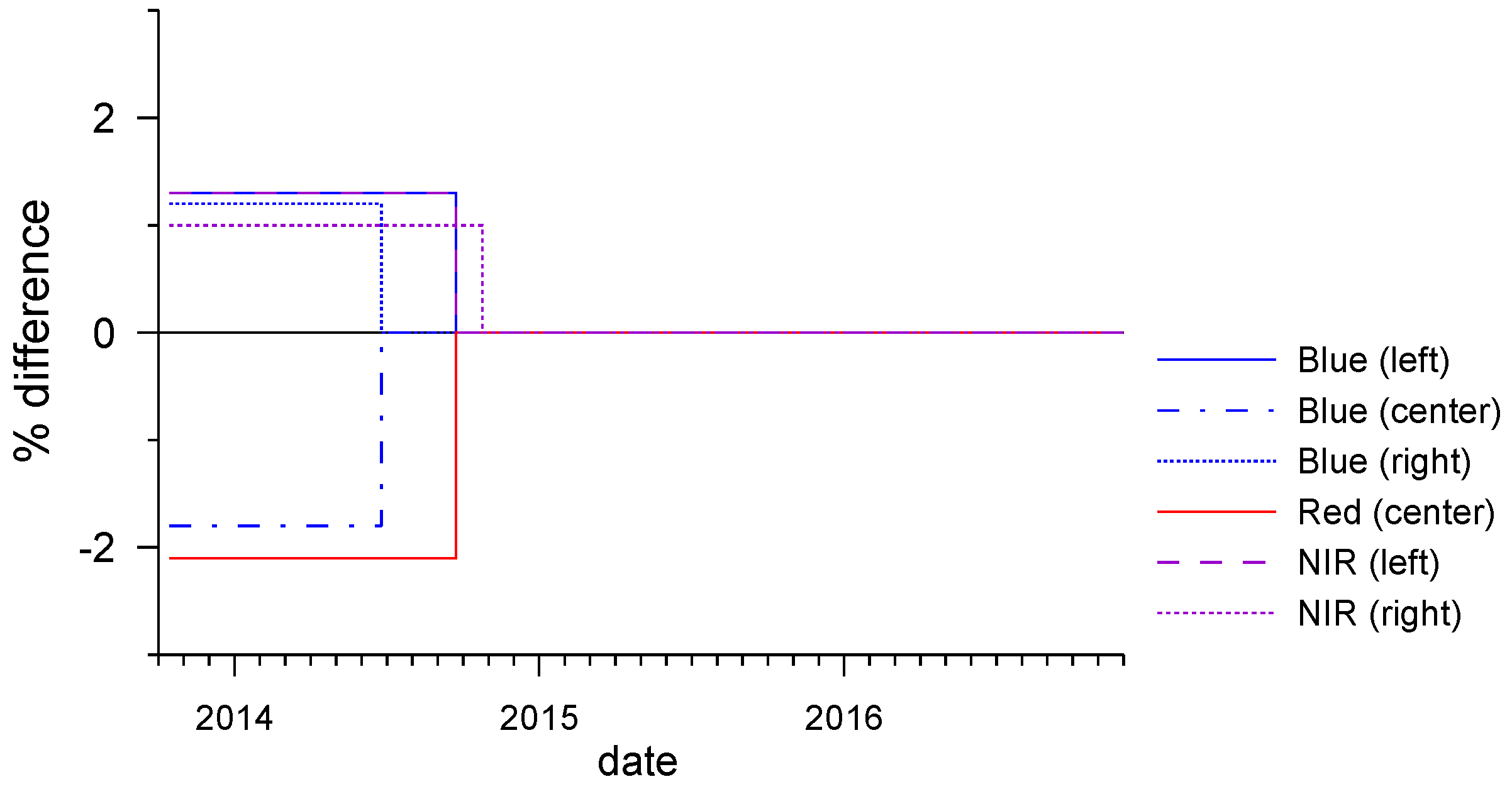
2.1.1. Inter-Camera Adjustments of VNIR Absolute Calibration Coefficients

The PROBA-V instrument is composed of three separate cameras, with an overlap of about 75 visible and near infrared (VNIR) pixels between the left and the center camera and between the center and right cameras, respectively. For the camera-to-camera bias assessment, the overlap region between two adjacent cameras was exploited [17]. In order to improve the consistency between the three PROBA-V cameras, adjustments to the absolute calibration coefficients of the VNIR strips were implemented within the C0 near-real time (NRT) processing chain to correct for a band dependent camera-to-camera bias (Figure 1). More specifically, on 26 June 2014, a 1.8% reduction in radiance for the blue center strip and a 1.2% increase in radiance for the blue right strip were applied. Furthermore, on 23 September 2014 a reduction of 2.1% to the red center radiance, a 1.1% increase to the blue left radiance and a 1.3% increase to the near infrared (NIR) left radiance were performed. Finally, on 25 October 2014, the right NIR radiance was increased by 1%. In order to have a consistent adjustment of the camera-to-camera bias along the full mission, it was decided to apply these coefficients from the start of the mission as part of the C1 reprocessing, allowing therefore to remove the stem-wise corrections introduced in the NRT processing (see Figure 1).

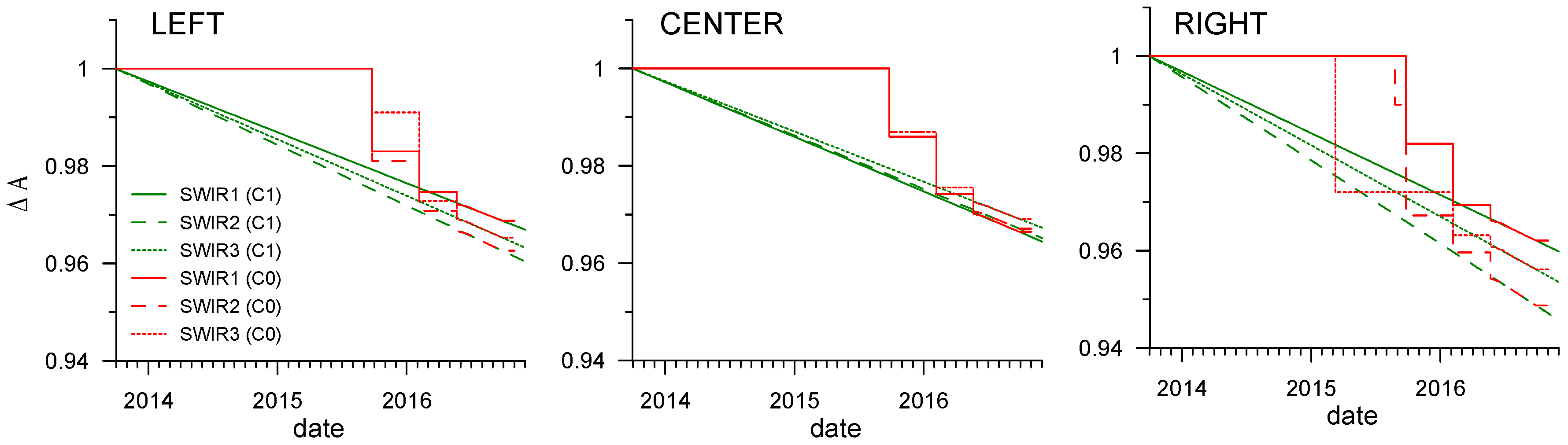
2.1.2. Degradation Model for SWIR Absolute Calibration Coefficients

Calibration over the Libya-4 desert site is used by the Image Quality Center (IQC) of PROBA-V to monitor the stability of the spectral bands and cameras of the instrument [17,18]. The approach relies on comparing the cloud-free TOA reflectance as measured by PROBA-V with modeled TOA reflectance values calculated following Govaerts et al. [19]. The long-term monitoring of the ratio (model/measurement) over these spectrally and radiometrically-stable desert sites allows for the estimation of the detector responsivity changes with time. For the VNIR strips, the detector response degradation is not significant during the first three years of the mission and well within the accuracy of the approach [17,18]. In contrast, for the short-wave infrared (SWIR) detectors a more significant degradation is observed: between −0.9% and −1.5% per year. PROBA-V has nine SWIR strips: each PROBA-V camera has a SWIR detector consisting of three linear detectors or strips of 1024 pixels, referred to as SWIR1, SWIR2, and SWIR3. In C0, the SWIR detector degradation was corrected using a step-wise adjustment of the SWIR absolute calibration coefficients (A_SWIR). In C1, this is replaced by a degradation model: a linear trending model is fitted to the OSCAR desert vicarious calibration results obtained for the nine different SWIR strips (Figure 2).

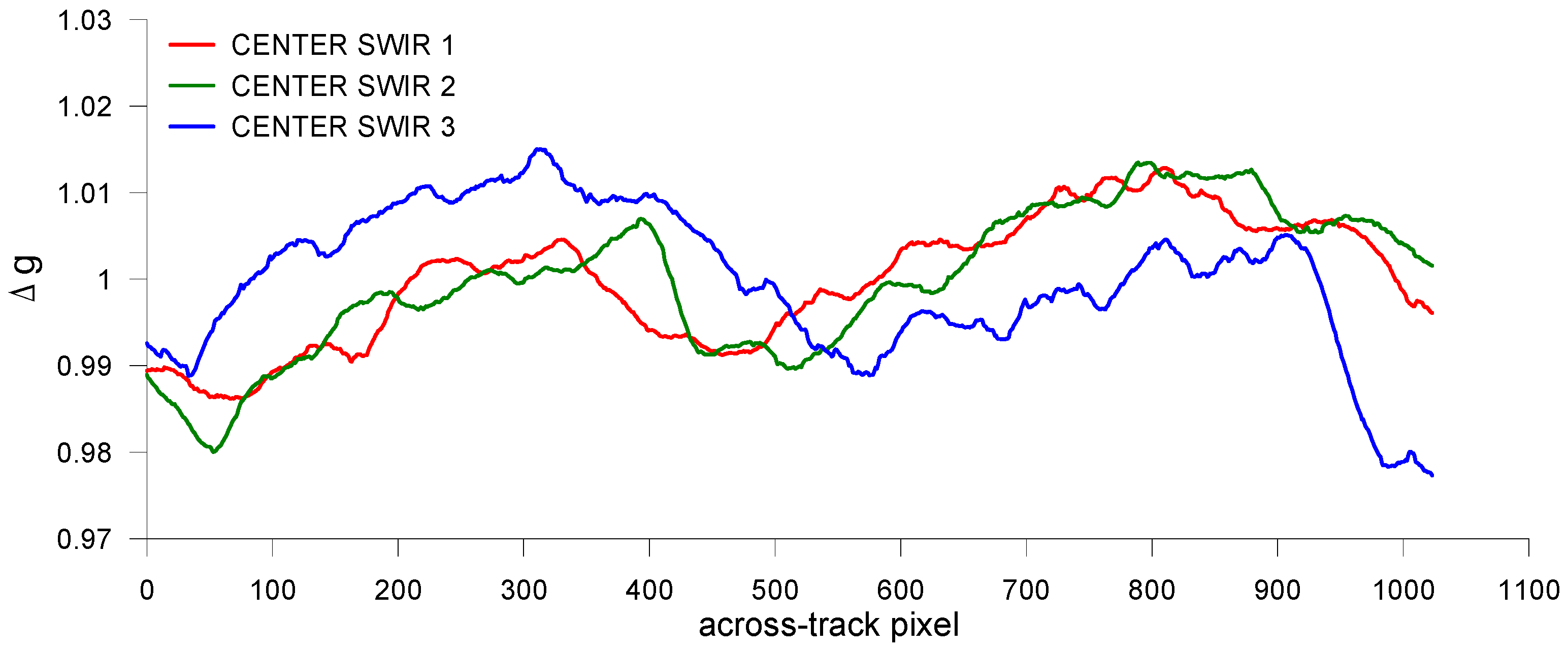
2.1.3. Improvement of Multi-Angular Calibration of the Center Camera SWIR Strips

The distribution of the cameras with butted SWIR detectors and the lack of on-board diffusers for flat-fielding purposes makes in-flight correction for non-uniformities in the field-of-view of the instrument a challenging issue. In order to better characterize and correct for non-uniformities, PROBA-V performed a 90° yaw maneuver over the Niger-1 desert site on 11 April 2016. In this 90° yaw configuration, the detector array of the CENTER camera runs parallel to the motion direction and a given area on the ground is subsequently viewed by the different pixels of the same strip (Figure 3). Improved low frequency multi-angular calibration coefficients for the SWIR strips of the center camera have been derived from this yaw maneuver data. Figure 4 shows the changes to equalization coefficients for the three SWIR strips of the center camera. The equalization updates were applied to the instrument calibration parameters (ICP) in C0 since June 2016, while for C1 the equalization coefficients of the center SWIR strips are corrected for the whole archive.

2.1.4. Dark Current and Bad Pixels

The dark current correction of PROBA-V C0 data acquired before 2015 was based on dark current acquisitions over oceans during nighttime with a very long integration of 3 s. This resulted in detector saturation and/or non-linearity effects for some SWIR pixels with a very high dark current. In C1, the dark current values of these saturated pixels are replaced with the dark current value retrieved from dark current acquisitions performed with lower integration time.

Furthermore, the ICP files are corrected for a bug found in the code for the final *.xml formatted ICP file generation. Before January 2015, this caused the assignment of the dark current to the wrong pixel ID in the C0 ICP files. Finally, in reprocessing mode, dark current values in the ICP files are based on the dark current acquisitions of the applicable month, while in the near-real time processing the dark current values are based on the previous month.

A minor change is made to the date of the assignment of the status ‘bad’ in the ICP files. For the reprocessing, an ICP file is generated at the start of each month. A pixel which became bad during that month is declared ‘bad’ in the C1 ICP file at the start of a month, aligned with the starting date of an ICP update.

2.2. Geometric Calibration

As with any operational sensor, PROBA-V exhibits perturbations relative to the ideal sensor model. These perturbations are caused by optical distortions, thermal related focal plane distortions or exterior orientation inaccuracies. Since the start of the PROBA-V nominal operations, in-orbit geometric calibration is applied in order to ensure a high geometric quality of the end products. The exterior orientation (i.e., boresight misalignment angles) and interior orientation deformations at different conditions (e.g., temperature, time exit from eclipse) are continuously monitored and estimated, with the objective to update the ICP files when necessary. Geometric calibration is performed by an autonomous in-flight software package, using the Landsat Global Land Survey (GLS) 2010 [20] Ground Control Point (GCP) dataset.

In C0 and C1, there are slight differences in the implementation date of consecutive updates to geometric ICP files.

Table 1. Overview of creation date and validity period for updated geometric ICP files for the period November 2013–November 2016. In C0, the validity period runs from ‘creation date’ till ‘end validity’, while in C1 the validity period runs from ‘start validity’ to ‘end validity’. The geometric error reduction is the difference between new and old geometric error, normalized over the old geometric error (in %).

Creation Date	Start Validity	End Validity	Geometric Error Reduction (%)
			Blue	Red	NIR	SWIR
8 September 2016	1 September 2016		−26.9	−33.7	−24.9	−23.9
16 February 2016	8 February 2016	1 September 2016	−80.2	−85.7	−91.8	−77.4
25 January 2016	19 January 2016	8 February 2016	−38.9	−46.0	−35.6	−29.3
2 November 2015	27 October 2015	19 January 2016	−72.3	−67.9	−59.0	−60.1
6 October 2015	3 October 2015	27 October 2015	−34.9	−42.7	−36.7	−34.9
9 July 2015	4 July 2015	3 October 2015	−68.2	−74.1	−54.3	−30.3
6 May 2015	20 April 2015	4 July 2015	−74.7	−84.0	−102.8	−93.7
24 March 2014	12 March 2014	20 April 2015	−87.5	−90.8	−90.2	−92.5
7 January 2014	1 January 2014	12 March 2014	−75.3	−93.5	−110.3	−98.6
9 November 2013	1 November 2013	1 January 2014	N/A	N/A	N/A	N/A
28 November 2013	16 October 2013	1 November 2013	N/A	N/A	N/A	N/A

gives an overview of the creation date and validity period for geometric ICP file updates and the associated geometric error reduction. The geometric calibration updates result in an average geometric error reduction of 64.5% from January-2014 onwards. In the period before, no error reduction is expected since the data suffers from random geometric error caused by an issue in the onboard star tracker. In the nominal processing, updated ICP files are applied from the ‘creation’ date onwards. In the reprocessing workflow, updates are applied from the ‘start validity’ date. This difference causes small geometric shifts between C0 and C1 in the period between the ‘start validity’ and ‘creation’ date.

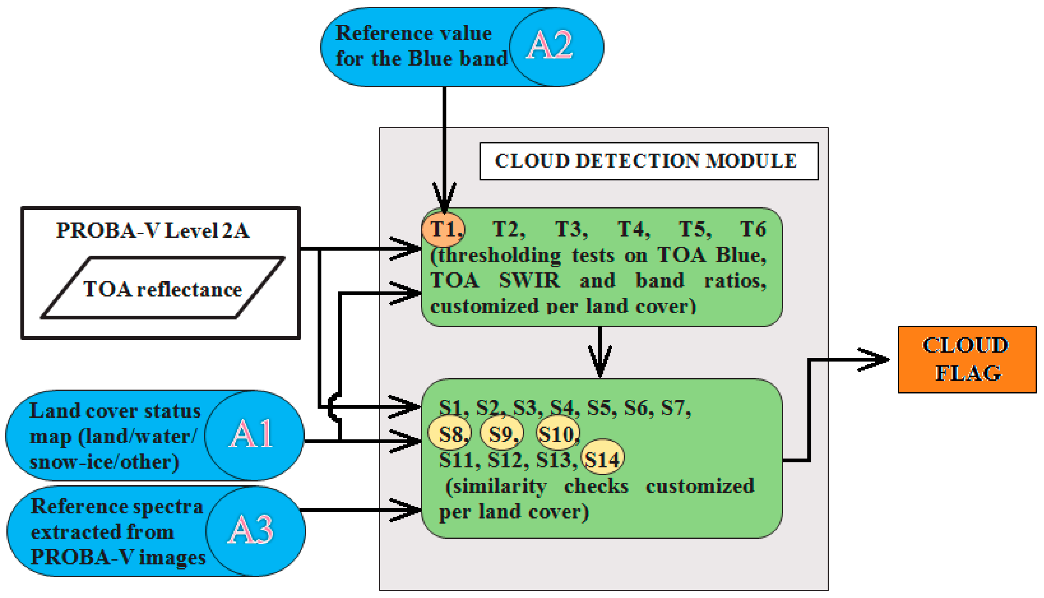
2.3. Cloud Detection

In PROBA-V C0, cloud detection was performed as in the SPOT-Vegetation processing chain [21]: the cloud cover map was derived as a union of two separate cloud masks, derived from the Blue and SWIR bands by using a simple thresholding strategy [4]. One of the main motivations for the C1 reprocessing was to address the cloud detection issues in the C0 dataset as reported by several users: (i) an overall under-detection of clouds, in particular for optically thin clouds, with resulting remaining cloud contamination in the composite products; and (ii) a systematic false detection over bright targets. In order to tackle the observed drawbacks, a completely new cloud detection algorithm was designed for C1, moving from a static threshold technique to an adaptive threshold approach. Similar to the old algorithm, the output of the new cloud masking algorithm in C1 is a binary mask in which every PROBA-V pixel is marked as ‘cloud’ or ‘clear’.

The new algorithm introduces major changes in two aspects (Figure 5): (i) the use of ancillary maps as reference data; and (ii) the application of customized tests, according to the land cover status of the pixel. The tests include threshold tests on TOA Blue, TOA SWIR and band ratios, and similarity checks based on the Spectral Angle Distance (SAD) between the pixel spectrum and reference spectra [22].

The PROBA-V C1 cloud detection algorithm is illustrated in Figure 5. Three types of auxiliary data (A1–A3 in Figure 5) are used as input: (i) monthly land cover status maps at 300 m resolution derived from the ESA Climate Change Initiative (CCI) Land Cover project [23]; (ii) monthly background surface reflectance climatology built from the MERIS full resolution 10-year archive, complemented with albedo maps from the GlobAlbedo project [23]; and (iii) reference PROBA-V spectra for specific land/cloud cover types.

Firstly, the land cover status maps label each pixel for each month of the year into one of the following classes: ‘land’, ‘water’, ‘snow/ice’, and ‘other’. For each of these classes, a customized set of cloud detection tests was defined. In a second step, monthly background surface reflectance climatology reference maps for the blue band, generated from the MERIS archive in the frame of the ESA CCI Land Cover project [23] are used. The monthly averages are derived from the seven-daily surface reflectance time series of the two blue MERIS bands (413 and 443 nm), over the period 2003–2012, with a spatial resolution of 300 m. Data gaps were completed with broadband (300–700 nm) albedo values provided by the GlobAlbedo project [24] at a spatial resolution of 5 km. For pixels having the status equal to ‘land’, ‘water’, or ‘other’, a first separation between cloudy and clear pixels is done by a simple thresholding applied to the difference between the actual blue reflectance and the reference value (indicated by T1 in Figure 5). Following the thresholding test for the reflectance in the blue band, a series of customized tests are designed for each distinct pixel status, including thresholding on SWIR reflectance and band ratios (T2 to T6). The tests may be active or inactive, depending on the pixel status, and the thresholds are tuned for each status value.

Finally, similarity tests are applied to check the SAD between the current pixel and a set of pre-defined reference spectra extracted as average spectra of a large number of PROBA-V pixels belonging to the same type of surface (e.g., deep sea water), generated from the training database (see below). Out of the 14 similarity checks (S1 to S14), 4 are common to all observed spectra and use equal thresholds across pixel statuses (S8, S9, S10, and S14). The remaining similarity checks may be active or not, with tuned thresholds, depending on the pixel status. For the complete list of the tests and their corresponding thresholds, the reader is referred to the PROBA-V Products User Manual [6]. After all tests are completed, the algorithm outputs the computed cloud flag.

Thresholds were tuned to maximize the overall accuracy of the algorithm, while keeping a good balance between missed clouds and clear pixels erroneously marked as clouds, with respect to a training dataset of over 43,000 manually labeled pixels classified in three cloud cover classes: ‘totally cloudy’ (6000 spectra), ‘semi-cloudy’ (16,277 spectra), and ‘clear sky’ (21,200 spectra). The training database was extracted from four daily global PROBA-V composites for the following days: 21 March 2014, 21 June 2014, 21 September 2014, and 21 December 2014. Each pixel was also assigned to one of the following land cover classes: ‘dark water (ocean)’, ‘dark water (inland)’, ‘turbid water’, ‘desert/bare soil’, ‘vegetation’, ‘wetland’, ‘salt’, ‘urban’, and ‘snow/ice’. Training pixels were well distributed over the globe and all land cover classes were represented in the three cloud cover classes.

2.4. Other Differences between C0 and C1 and Issues Solved

During the C0 nominal processing, two bugs were detected and fixed. Logically, the bug fixes are applied on the complete C1 archive. The first bug fix (implemented in C0 on 16 July 2015) limits the impact of on-board compression errors. Before the fix, entire segments of spectral band data were omitted after a decompression error, which happened on a random basis every few days. The fix limits the amount of missing data in the final L1C, L2A, and synthesis product lines to the block where the decompression error occurred. The second bug fix (implemented in C0 on 10 February 2016) is related to the satellite attitude data check, causing some segment data to be wrongfully marked as ‘no data’. All data lost in C0 before the implementation date have been successfully compiled into the C1 collection.

An issue related to leap second implementation was identified in the C0 nominal processing: an incorrect leap second value was applied during the period 23 April 2015 until 29 June 2015. All telemetry data (satellite position, velocity, and attitudes) during this period was consequently timestamped with 1 s inaccuracy leading to an on-ground geolocation error of about 6 km. This was corrected for in C1, resulting in geometric shifts between the two collections for this period.

Finally, metadata of the delivered C1 products are compliant to the Climate and Forecast (CF) Metadata Conventions (v1.6) [25]. In C0, metadata were only compliant with these conventions starting from 6 January 2016.

3. Materials and Methods

3.1. Data Used

3.1.1. PROBA-V Collection 1 Level 2A

For the validation of the cloud detection, 61 Level 2A segment products (i.e., projected TOA reflectances) were used, with acquisition dates on 21 March 2015, 21 June 2015, 21 September 2015, and 21 December 2015. Note that these dates are different from the ones used for training dataset collection, which allows for a completely independent validation of the cloud screening algorithm.

3.1.2. PROBA-V Collection 0 and Collection 1 Level 3 S10-TOC

For the evaluation of the PROBA-V Collection 1 archive, a 37 months period (1 November 2013 until 30 November 2016) of S10 TOC reflectance and NDVI of PROBA-V C0 and C1 at 1 km were considered, i.e., 111 10-daily composites. Unclear observations are flagged as ‘cloud/shadow’, ‘snow/ice’, ‘water’, or ‘missing’, based on the information contained in the status map (SM).

3.1.3. SPOT/VGT Collection 2 and Collection 3 Level 3 S10-TOC

For the comparison with an external dataset from METOP/AVHRR (see below), the PROBA-V C0 and C1 are extended backward in time, using S10 TOC reflectance and NDVI at 1 km resolution of the SPOT/VGT Collection 2 (C2) and Collection 3 (C3). After the end of the SPOT/VGT mission in May 2014, the data archive from both the VGT1 and VGT2 instruments was reprocessed, aiming at improved cloud screening and correcting for known artefacts such as the smile pattern in the VGT2 blue band and the Sun–Earth distance bug in TOA reflectance calculation [2]. SPOT/VGT-C3 was proven to be more stable over time compared to the previous SPOT/VGT-C2 archive.

The time series from SPOT/VGT-C2 and SPOT/VGT-C3 considered here runs from January 2008 until December 2013. In the comparison with METOP/AVHRR, the switch from SPOT/VGT to PROBA-V data is set on January 2014.

3.1.4. METOP/AVHRR

The European Organisation for the Exploitation of Meteorological Satellites (EUMETSAT) Polar System (EPS) consists of a series of polar orbiting meteorological satellites. METOP has a local stable overpass time at around 9:30 h. The AVHRR-instrument onboard METOP is used to generate 10-daily NDVI by the LSA-SAF (http://landsaf.meteo.pt). The AVHRR S10 TOC surface reflectance and NDVI are processed in a very similar way to those of PROBA-V, with the same water vapor and ozone inputs, and a similar atmospheric correction and compositing method [26]. There are however differences in calibration, cloud detection, and overpass time stability. Global data from METOP-A (launched in 2006) for the period January 2008–November 2016 are used in the comparison.

3.2. Sampling

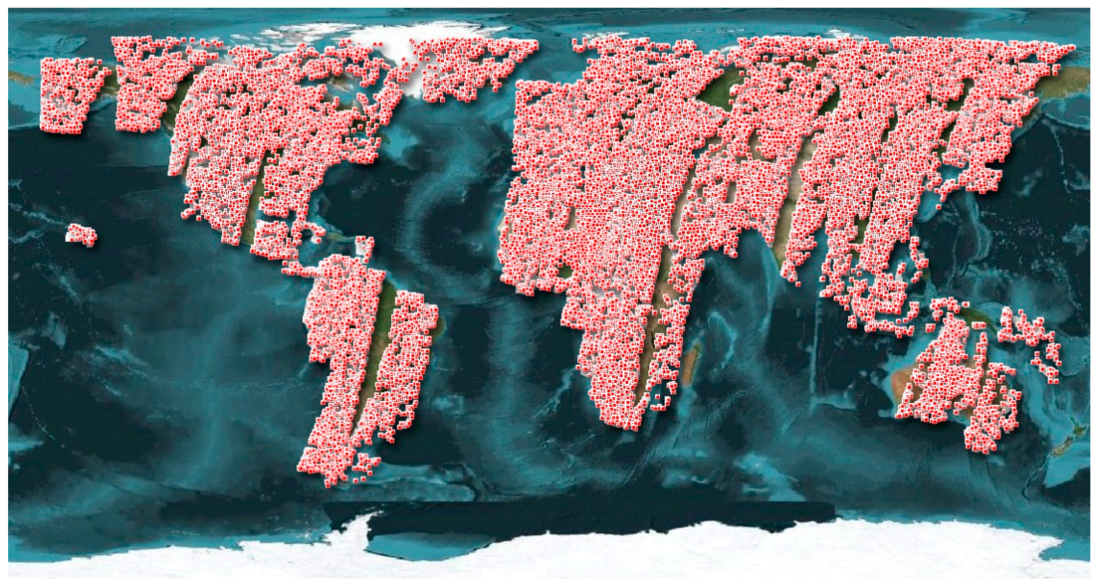
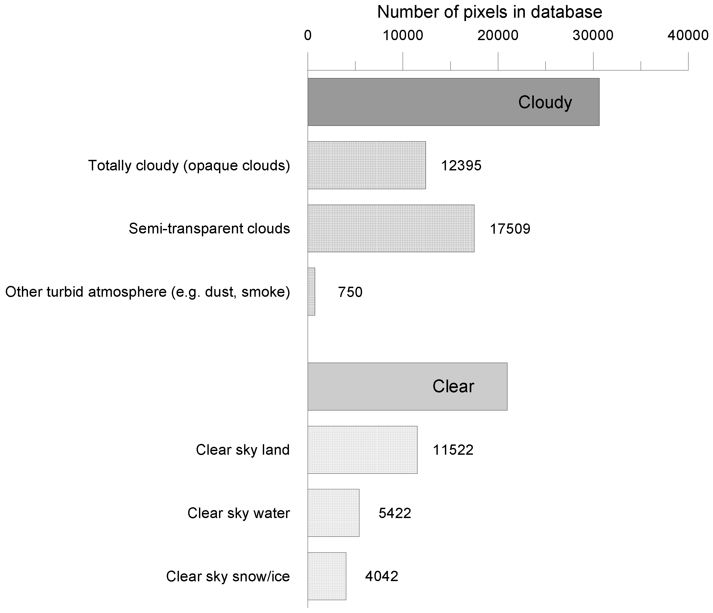
3.2.1. Validation Database for Cloud Detection

The validation database for cloud detection contains almost 53,000 pixels (Figure 6 and Figure 7). All pixels are manually collected, classified, and labeled by a cloud pixel expert as (i) cloud: totally cloudy (opaque clouds), semi-transparent cloud, or other turbid atmosphere (e.g., dust, smoke); or (ii) clear: clear sky water, clear sky land, or clear sky snow/ice. The semi-transparent clouds were further differentiated through visual assessment into three density classes, which enables to understand which categories of semi-transparent clouds are captured by the cloud detection algorithm during the validation process: (i) thick semi-transparent cloud; (ii) average or medium dense semi-transparent cloud; and (iii) thin semi-transparent cloud.

3.2.2. Global Subsample

In order to reduce processing time, a global systematic subsample is taken over the global images by taking the central pixel in each arbitrary window of 21 by 21 pixels. For the pairwise comparison between C0 and C1, pixels identified in both SM as ‘clear’ are selected, and only observations with an identical observation day (OD) are considered. In order to discriminate between the three different PROBA-V cameras, additional sampling is based on thresholds on the viewing zenith angle (VZA) and viewing azimuth angle (VAA) of each VNIR observation (

Table 2. Thresholds on VNIR VZA and VAA to discriminate between left, center, and right cameras.

	LEFT	CENTER	RIGHT
VZA (VNIR)	>20°	<18°	>20°
VAA (VNIR)	<90° OR >270°		between 90° and 270°

). As a result, C0 and C1 surface reflectance and NDVI that are derived from identical clear observations are compared.

3.3. Methods

3.3.1. Validation of the Cloud Detection Algorithm

The cloud detection algorithm is validated through visual inspection of the cloud masks and through pixel-by-pixel comparison with the validation database. The accuracy of the method is assessed by measuring the agreement between the cloud algorithm output and the validation dataset. A confusion matrix is used to derive the overall accuracy (OA), user’s accuracy (UA), producer’s accuracy (PA), commission error (CE), and omission error (OE). The OA is computed as the ratio of the sum of all correctly-classified pixels on the sum of all validation pixels. The UA for a specific class is the ratio between correctly-classified pixels and all pixels classified as the specific class, where CE = 100% − UA. The PA for the specific class is the fraction of correctly-classified pixels and all ground truth class pixels, and OE = 100% − PA. In order to assess the overall classification, Krippendorf’s α is derived [27], which accounts for agreement by chance and is scaled from zero (pure chance agreement) to one (no chance agreement) [28]. For the visual inspection, false color composites of image subsets are overlaid with the cloud (and snow/ice) mask.

3.3.2. Spatio-Temporal Variation of Validation Metrics

In order to evaluate the temporal evolution of the intercomparison of surface reflectance and NDVI between two datasets, a number of validation metrics (

Table 3. Validation metrics used to compare two datasets.

Abbreviation	Metric	Formula 1
GMR slope	Geometric mean regression slope	$b=sign\left(R\right)\frac{{\sigma }_Y}{{\sigma }_X}$
GMR intercept	Geometric mean regression intercept	$a=Y-b·X$
R2	Coefficient of determination	$R^2={\left(\frac{{\sigma }_{X,Y}}{{\sigma }_X·{\sigma }_Y}\right)}^2$
MSD	Mean squared difference	$MSD=\frac{1}{n}{\displaystyle {\displaystyle \sum }_{i=1}^n}{\left(X_i-Y_i\right)}^2$
RMSD	Root-mean-squared difference	$RMSD=\sqrt{\frac{1}{n}{\displaystyle {\displaystyle \sum }_{i=1}^n}{(X_i-Y_i)}^2}$
RMPDu	Root of the unsystematic or random mean product difference	$RMP{D}_u=\sqrt{\frac{1}{n}{\displaystyle {\displaystyle \sum }_{i=1}^n}(|X_i-{\widehat{X}}_i|)(|Y_i-{\widehat{Y}}_i|)}$
RMPDs	Root of the systematic mean product difference	$RMP{D}_s=\sqrt{MSD-MP{D}_u}$
MBE	Mean bias error	$MBE=\frac{1}{n}{\displaystyle {\displaystyle \sum }_{i=1}^n}\left(X_i-Y_i\right)$

¹${\sigma }_X$ and ${\sigma }_Y$ are the standard deviations of X and Y, ${\sigma }_{X,Y}$ is the covariance of X and Y, $R$ is the correlation coefficient, $sign()$ takes the sign of the variable between the brackets, ${\widehat{X}}_i$ and ${\widehat{Y}}_i$ are estimated using the GMR model fit and $n$ is the number of samples.

) are calculated for each time step. The linear relationship between two datasets is identified based on a geometric mean regression (GMR) model [29]. Other metrics are the root-mean-squared difference (RMSD), the root systematic and unsystematic mean product difference (RMPDs and RMPDu), all three expressed in the same unit as the datasets themselves (% for TOC reflectance or unitless for NDVI), and the mean bias error (MBE). To perform a combined assessment of the spatial and temporal variability of the metrics, Hovmöller diagrams are based on data intercomparison for each time step and for each latitude band of 6°.

4. Results and Discussion

4.1. Cloud Detection

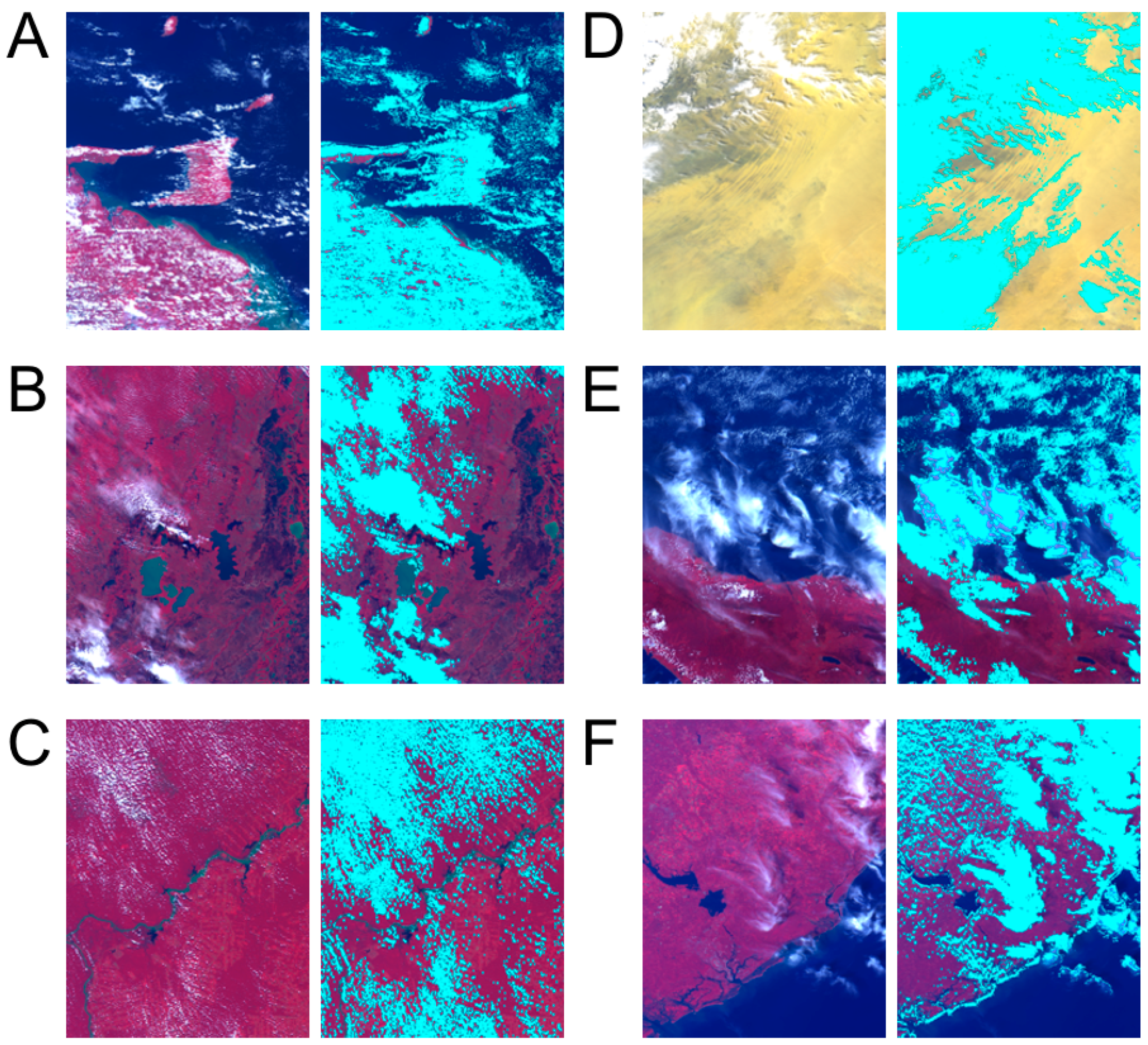
4.1.1. Qualitative Evaluation

Overall, visual inspection of the cloud masking result shows good detection of opaque and semi-transparent clouds. Figure 8 shows six examples that demonstrate the behavior of the algorithm over different surfaces (vegetated areas, bare surface, different water types, and snow/ice) and with different cloud types (opaque clouds, small cumulus clouds, semi-transparent clouds). A number of flaws in the cloud detection algorithm are illustrated: overdetection of clouds (Figure 8A,C,D); turbid waters detected as ‘cloud’ (Figure 8A,B,F); underdetection of semi-transparent clouds over water surfaces (Figure 8E), bright coastlines detected as cloud (Figure 8F). Some other issues (not shown here) are that sun glint or ice on water surfaces are sometimes incorrectly detected as cloud. Finally, the qualitative evaluation has revealed that thick clouds are sometimes wrongly classified as snow/ice. In some cases, this is combined with saturation of one or more PROBA-V bands. The snow detection algorithm has not changed between C0 and C1.

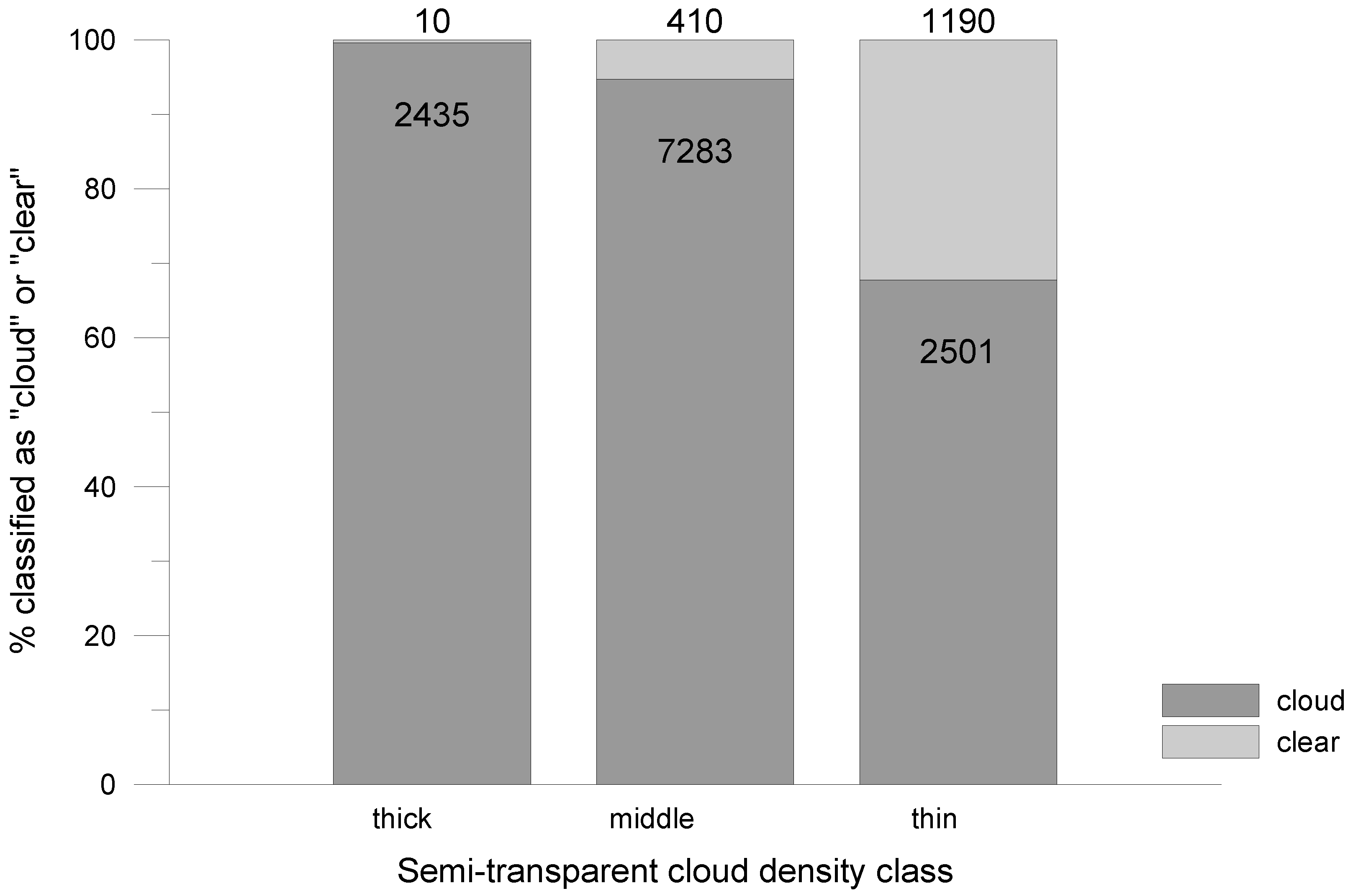
4.1.2. Quantitative Evaluation

Table 4. Confusion matrices for (A) all surfaces, (B) land, and (C) water. The ‘cloud’ class includes semi-transparent clouds.

A. All surfaces, OA = 89.0%, α = 0.764
	Validation database
Cloud detection	Clear	Cloud	UA	CE
Clear	13,095	1655	88.8%	11.2%
Cloud	2934	24,140	89.2%	10.8%
PA	81.7%	93.6%
OE	18.3%	6.4%
B. Land, OA = 89.7%, α = 0.771
	Validation database
Cloud detection	Clear	Cloud	UA	CE
Clear	8633	782	91.7%	8.3%
Cloud	2273	18,069	88.8%	11.2%
PA	79.2%	95.9%
OE	20.8%	4.1%
C. Water, OA = 87.3%, α = 0.741
	Validation database
Cloud detection	Clear	Cloud	UA	CE
Clear	4462	873	83.6%	16.4%
Cloud	661	6071	90.2%	9.8%
PA	87.1%	87.4%
OE	12.9%	12.6%

shows the confusion matrices comparing the cloud detection algorithm result with the validation database, for all surfaces, and separately for land and water surfaces, respectively. The ‘cloud’ class includes opaque clouds and semi-transparent clouds. Pixels flagged as ‘snow/ice’ or ‘missing’ are excluded from the analysis.

The OA yields 89.0% (over all surfaces), 89.7% (over land) and 87.3% (over water), indicating the cloud detection algorithm is slightly more accurate over land than over water. This is also reflected in Krippendorf’s α, which reaches 0.764 (all surfaces), 0.771 (land) and 0.741 (water). For ‘cloud’, the PA is very high over all surfaces (93.6%) and over land (95.9%), indicating clouds are detected with very little omission errors, related to the fact that the cloud detection scheme is cloud conservative. For these cases, OE for ‘clear’ is relatively high. Differently, OE for ‘clear’ and ‘cloud’ is similar over water.

Additionally, it has been investigated how the algorithms behave with respect to semi-transparent clouds. Figure 9 shows how the three density classes of semi-transparent clouds are classified by the algorithms and answers the question if a semi-transparent cloud is classified as cloud or as clear. This depends on whether the semi-transparent cloud was thin, middle or thick. The light colors indicate the percentage of pixels classified as ‘cloud’, the dark color indicates the percentage of pixels classified as ‘clear’. The figure shows that the thick semi-transparent clouds are almost all classified as ‘cloud’ while from the thin semi-transparent clouds a larger portion is classified as ‘clear’.

4.1.3. Effect on S10 Product Completeness

The adapted cloud screening has implications for the amount of clear vs. unclear observations over land in the TOC-S10 C0 and C1 archives. For the period November 2013–November 2016, the average amount of missing observations (due to illumination conditions or bad radiometric quality) remains unchanged between C0 and C1 (

Table 5. Status map labelling in S10-TOC 1 km in PROBA-V C0 and C1 (% land pixels, November 2013–November 2016) and difference between C0 and C1.

Label	PROBA-V C0 S10-TOC 1 km	PROBA-V C1 S10-TOC 1 km	Difference
Clear	79.3%	74.0%	−5.4%
Not clear	20.7%	26.0%
Missing	6.3%	6.3%	−0.0%
Cloud/shadow	2.3%	14.1%	+11.8%
Snow/ice	12.1%	5.6%	−6.5%

). However, a larger amount of clouds/shadows is detected (+11.8%), and as a consequence there are less clear observations in C1 there (−5.4%). Less pixels are detected as snow/ice (−6.5%).

4.2. Comparison between PROBA-V C0 and C1

The reprocessing causes differences between PROBA-V C0 and C1, but the magnitude of the difference is dependent on the time period. The temporal evolution of MBE and RMSD between PROBA-V C0 and C1 S10-TOC reflectance is shown in Figure 10. The MBE for the VNIR bands remains in the range (−0.4%, 0.4%) but confirms sudden changes in the period October 2013–October 2014, which are in agreement with the updates applied to VNIR absolute calibration in C0. The temporal profile of the MBE for the NIR band shows a peak in the second dekad of November 2016. This larger difference between C1 and C0 is linked to a problem in C0 in the water vapor data used as input for the atmospheric correction of the images acquired on 20 November 2016. The issue was solved in C1. The MBE for the SWIR band clearly shows the degradation model application in C1, instead of the sudden changes in C0. The difference between C1 and C0 peaks in September 2015 with an MBE up to −0.6%. The temporal evolution of the RMSD shows periods with relatively larger difference between C1 and C0, related to the different implementation date of updates to the geometric calibration and the incorrect leap second implementation in C0 (23 April 2015 until 29 June 2015).

Figure 11 illustrates the temporal evolution of the global difference between C0 and C1 S10-TOC NDVI for the same period. The updates of the RED and NIR absolute calibration parameters are clearly reflected in the temporal evolution of the MBE. Changes in the ICP files causes the RMSD to fluctuate roughly between 0.005 and 0.015. The different implementation date of updates to the geometric calibration and the corrected leap second implementation has a relatively large effect on the RMSD, with peaks up to 0.02.

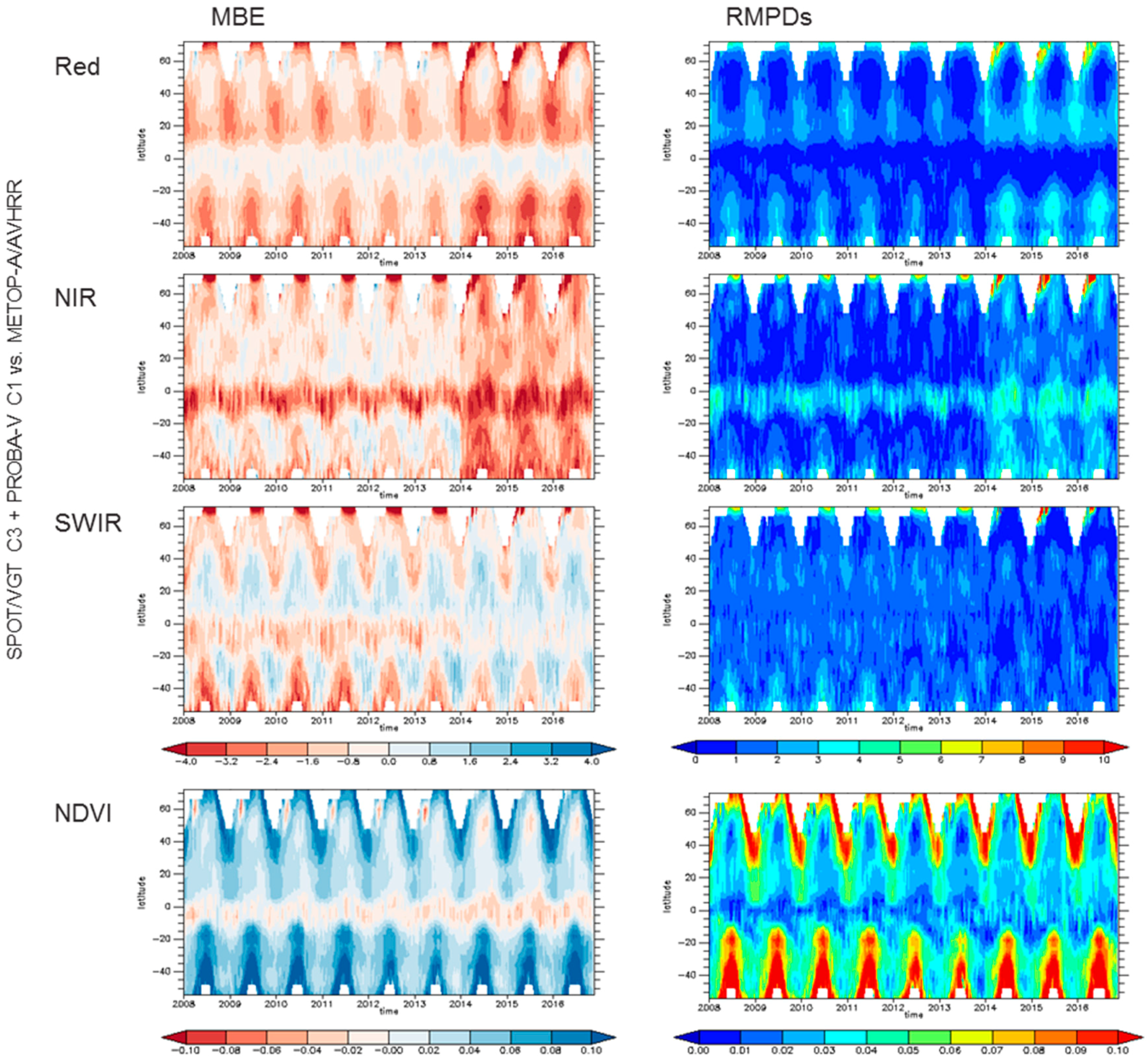
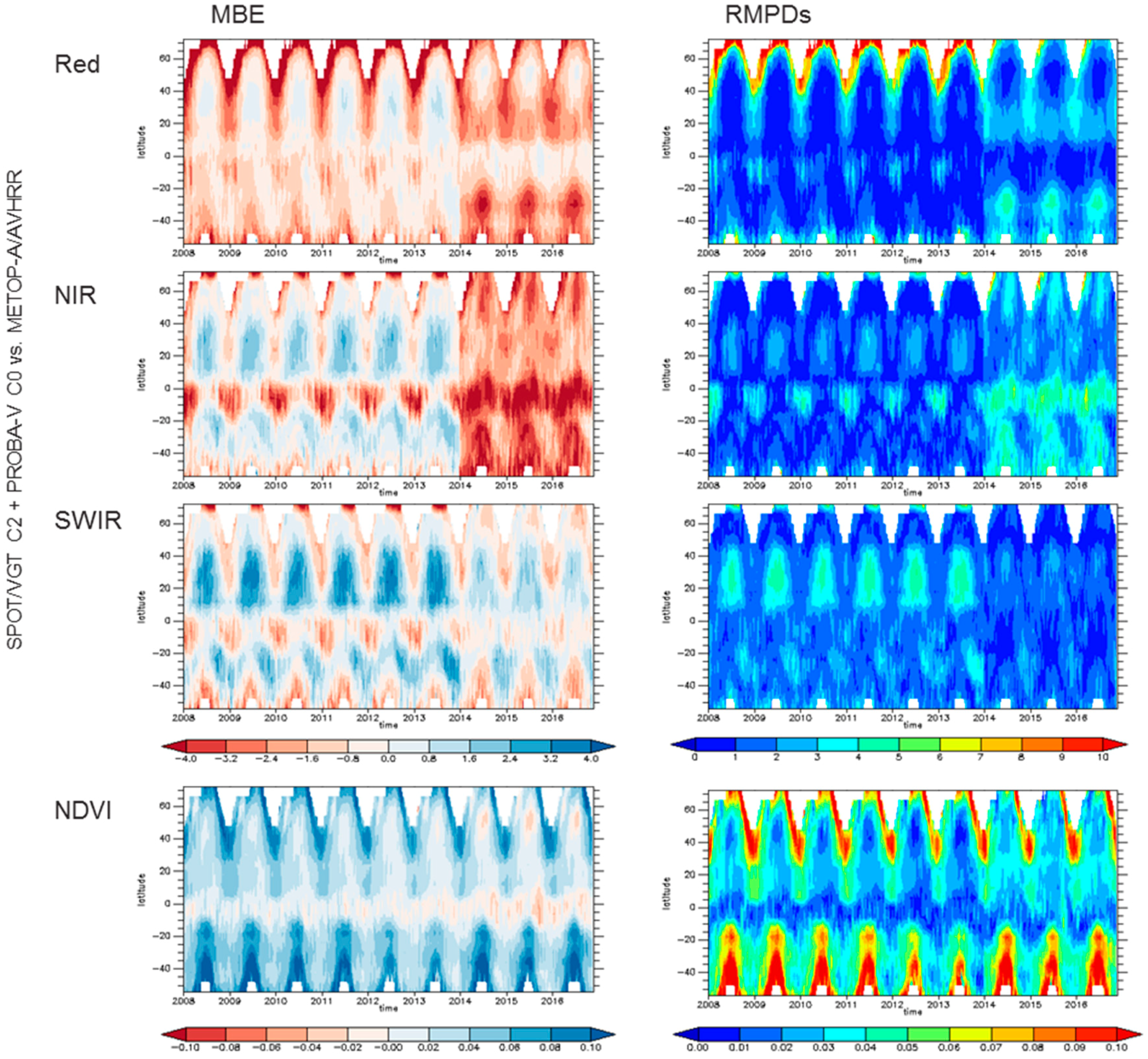
4.3. Comparison to METOP/AVHRR

The previous sections focused on the effect of the reprocessing on the PROBA-V dataset. Now the combined SPOT/VGT and PROBA-V time series are compared to an external dataset: the spatio-temporal patterns of the differences between the combined SPOT/VGT and PROBA-V time series before and after their last reprocessing and the external dataset from METOP/AVHRR allows us to evaluate the effect of the reprocessing campaigns on the temporal stability. Of course, there are intrinsic differences between combined TOC reflectance or NDVI datasets derived from SPOT/VGT and PROBA-V on the one hand, and METOP/AVHRR on the other hand, most importantly linked to differences in overpass time, spectral response functions, radiometric calibration and image processing (e.g., cloud detection and atmospheric correction). It is to be noted that differences also exist between SPOT/VGT and PROBA-V, although the PROBA-V mission objective was to provide continuation to the SPOT/VGT time series: there are small differences in spectral response functions, both sensors were not radiometrically intercalibrated, and there is an important overpass time lag of about 45 min between SPOT/VGT at the end of its lifetime and PROBA-V.

Figure 12 illustrates the spatio-temporal behavior of the validation metrics between the combined series of SPOT/VGT-C3 and PROBA-V-C1 and METOP/AVHRR for the three common spectral bands (red, NIR, and SWIR) and the NDVI. The Hovmöller plots indicate a low inter-annual variation, hence stable bias between SPOT/VGT-C3–PROBA-V-C1 and METOP/AVHRR. The switch from SPOT/VGT to PROBA-V is however visible in the spatio-temporal plots, with relatively higher differences for Red and NIR after January-2014. This is related to the relatively larger differences in overpass time between PROBA-V and METOP-A, hence larger differences in illumination angles, which impacts especially the red and NIR directional reflectance [30]. Overall, the intra-annual and spatial variation are linked to differences in vegetation cover within the year (i.e., seasonality of vegetation densities at mid latitudes) and over the globe (e.g., high vegetation densities in the tropics). For red reflectance, the lowest MBE and RMPDs are observed in the tropics and in mid-latitude summers, related to lower red reflectance when vegetation densities are high. The opposite pattern is observed for NIR reflectance, which increases with vegetation cover. For SWIR reflectance, spatio-temporal patterns are overall less pronounced. The NDVI shows highest bias in mid- and high-latitude winter periods, which is possibly related to the low accuracy of the atmospheric correction applied at high solar zenith angles [31,32].

In order to evaluate the effect of the reprocessing on spatio-temporal stability, the combined series of the former SPOT/VGT-C2 and PROBA-V-C0 archives is compared to METOP/AVHRR (Figure 13). The figures show a much larger spatio-temporal instability, and the switch from SPOT/VGT to PROBA-V is more pronounced.

5. Conclusions

This paper provides an overview of the modifications in the PROBA-V processing chain, and the related impacts on the new PROBA-V-C1 archive. The evaluation of the reprocessing is based on (i) qualitative and quantitative evaluation of the new cloud detection scheme; (ii) the relative comparison between PROBA-V-C0 and PROBA-V-C1 TOC-S10 surface reflectances and NDVI; and (iii) comparison of the combined SPOT/VGT and PROBA-V series with an external dataset from METOP/AVHRR.

The new cloud detection algorithm shows good performance, with an overall accuracy of 89.0%. The detection is slightly less performant over water (87.3%) than over land (89.7%). Since the algorithm is cloud conservative, clouds are detected with very little omission errors and many small clouds, cloud borders, and semi-transparent clouds are correctly identified. However, both the qualitative and quantitative evaluation has shown that there is an overdetection of clouds over bright surfaces (e.g., bright coastlines, sun glint, or ice on water surfaces and turbid waters). The adaptation of the cloud detection algorithm has resulted in less clear observations in C1 compared to C0 (−5.4%). A larger amount of clouds/shadows is detected (+11.8%), less pixels are labeled as snow/ice (−6.5%).

The temporal profile of the MBE between PROBA-V-C0 and PROBA-V-C1 blue, red, and NIR TOC reflectances show sudden changes in the period October 2013–October 2014, related to stepwise updates to the VNIR absolute calibration applied in C0, but the overall MBE remains within the range (−0.4%, 0.4%). The updates of the RED and NIR absolute calibration parameters are also clearly visible in the temporal evolution of the difference between C0 and C1 S10-TOC NDVI. The MBE remains within the range (−0.015, +0.015) and the RMSD varies between 0.005 and 0.02. The application of degradation models to the SWIR calibration in C1 results in more gradual differences between C0 and C1 SWIR TOC reflectance, with an MBE up to −0.6%. The different implementation date of updates to the geometric calibration, the incorrect leap second implementation in C0 (23 April 2015 until 29 June 2015) and a problem with the water vapor input data in C1 (20 November 2016) results in periods with relative larger RMSD between C0 and C1, although the RMSD remains well below 1%.

The spatio-temporal patterns of the bias between the combined series of SPOT/VGT-C3 and PROBA-V-C1 and an external dataset of red, NIR, and SWIR TOC reflectance and the NDVI derived from METOP-A/AVHRR indicate a relatively low inter-annual variation. Although the switch from SPOT/VGT to PROBA-V is visible, spatio-temporal behavior of the metrics show the recent reprocessing campaigns on SPOT/VGT (to C3) and PROBA-V (to C1) have resulted in a much more stable combined time series. The overpass time evolution for both (drifting) sensors causes bidirectional reflectance distribution function (BRDF) effects due to differences in illumination and viewing geometry.

References

1. Mellab, K.; Santandrea, S.; Francois, M.; Vrancken, D.; Gerrits, D.; Barnes, A.; Nieminen, P.; Willemsen, P.; Hernandez, S.; Owens, A.; et al. PROBA-V: An operational and technology demonstration mission-Results after decommissioning and one year of in-orbit exploitation. In Proceedings of the 4S (Small Satellites Systems and Services) Symposium, Porto Pedro, Spain, 26–30 May 2014. [Google Scholar]
2. Toté, C.; Swinnen, E.; Sterckx, S.; Clarijs, D.; Quang, C.; Maes, R. Evaluation of the SPOT/VEGETATION Collection 3 reprocessed dataset: Surface reflectances and NDVI. Remote Sens. Environ. 2017, 201, 219–233. [Google Scholar] [CrossRef]
3. Maisongrande, P.; Duchemin, B.; Dedieu, G. VEGETATION/SPOT: An operational mission for the Earth monitoring; presentation of new standard products. Int. J. Remote Sens. 2004, 25, 9–14. [Google Scholar] [CrossRef]
4. Dierckx, W.; Sterckx, S.; Benhadj, I.; Livens, S.; Duhoux, G.; Van Achteren, T.; Francois, M.; Mellab, K.; Saint, G. PROBA-V mission for global vegetation monitoring: Standard products and image quality. Int. J. Remote Sens. 2014, 35, 2589–2614. [Google Scholar] [CrossRef]
5. Sterckx, S.; Benhadj, I.; Duhoux, G.; Livens, S.; Dierckx, W.; Goor, E.; Adriaensen, S.; Heyns, W.; Van Hoof, K.; Strackx, G.; et al. The PROBA-V mission: Image processing and calibration. Int. J. Remote Sens. 2014, 35, 2565–2588. [Google Scholar] [CrossRef]
6. Wolters, E.; Dierckx, W.; Iordache, M.-D.; Swinnen, E. PROBA-V Products User Manual v3.0; VITO: Mol, Belgium, 2018. [Google Scholar]
7. Lambert, M.J.; Waldner, F.; Defourny, P. Cropland mapping over Sahelian and Sudanian agrosystems: A Knowledge-based approach using PROBA-V time series at 100-m. Remote Sens. 2016, 8, 232. [Google Scholar] [CrossRef]
8. Roumenina, E.; Atzberger, C.; Vassilev, V.; Dimitrov, P.; Kamenova, I.; Banov, M.; Filchev, L.; Jelev, G. Single- and multi-date crop identification using PROBA-V 100 and 300 m S1 products on Zlatia Test Site, Bulgaria. Remote Sens. 2015, 7, 13843–13862. [Google Scholar] [CrossRef]
9. Shelestov, A.; Kolotii, A.; Camacho, F.; Skakun, S.; Kussul, O.; Lavreniuk, M.; Kostetsky, O. Mapping of biophysical parameters based on high resolution EO imagery for JECAM test site in Ukraine. In Proceedings of the 2015 IEEE International Geoscience and Remote Sensing Symposium (IGARSS), Milan, Italy, 26–31 July 2015. [Google Scholar]
10. Baret, F.; Weiss, M. Algorithm Theoretical Basis Document—Leaf Area Index (LAI) Fraction of Absorbed Photosynthetically Active Radiation (FAPAR) Fraction of Green Vegetation Cover (FCover)-I2.01. GIO-GL Lot1, GMES Initial Operations. 2017. Available online: https://land.copernicus.eu/global/sites/cgls.vito.be/files/products/GIOGL1_ATBD_FAPAR1km-V1_I2.01.pdf (accessed on 25 February 2018).
11. Meroni, M.; Fasbender, D.; Balaghi, R.; Dali, M.; Haffani, M.; Haythem, I.; Hooker, J.; Lahlou, M.; Lopez-Lozano, R.; Mahyou, H.; et al. Evaluating NDVI Data Continuity Between SPOT-VEGETATION and PROBA-V Missions for Operational Yield Forecasting in North African Countries. IEEE Trans. Geosci. Remote Sens. 2016, 54, 795–804. [Google Scholar] [CrossRef]
12. Kempeneers, P.; Sedano, F.; Piccard, I.; Eerens, H. Data assimilation of PROBA-V 100 m and 300 m. IEEE J. Sel. Top. Appl. Earth Obs. Remote Sens. 2016, 9, 3314–3325. [Google Scholar] [CrossRef]
13. Sánchez, J.; Camacho, F.; Lacaze, R.; Smets, B. Early validation of PROBA-V GEOV1 LAI, FAPAR and FCOVER products for the continuity of the copernicus global land service. Int. Arch. Photogramm. Remote Sens. Spat. Inf. Sci. Arch. 2015, XL-7/W3, 93–100. [Google Scholar] [CrossRef]
14. Lacaze, R.; Smets, B.; Baret, F.; Weiss, M.; Ramon, D.; Montersleet, B.; Wandrebeck, L.; Calvet, J.C.; Roujean, J.L.; Camacho, F. Operational 333 m biophysical products of the copernicus global land service for agriculture monitoring. Int. Arch. Photogramm. Remote Sens. Spat. Inf. Sci. Arch. 2015, XL-7/W3, 53–56. [Google Scholar] [CrossRef]
15. Goor, E.; Dries, J.; Daems, D.; Paepen, M.; Niro, F.; Goryl, P.; Mougnaud, P.; Della Vecchia, A. PROBA-V Mission Exploitation Platform. Remote Sens. 2016, 8, 564. [Google Scholar] [CrossRef]
16. Sterckx, S.; Livens, S.; Adriaensen, S. Rayleigh, deep convective clouds, and cross-sensor desert vicarious calibration validation for the PROBA-V mission. IEEE Trans. Geosci. Remote Sens. 2013, 51, 1437–1452. [Google Scholar] [CrossRef]
17. Sterckx, S.; Adriaensen, S.; Dierckx, W.; Bouvet, M. In-Orbit Radiometric Calibration and Stability Monitoring of the PROBA-V Instrument. Remote Sens. 2016, 8, 546. [Google Scholar] [CrossRef]
18. Sterckx, S.; Adriaensen, S. Degradation monitoring of the PROBA-V instrument. GSICS Q. 2017, 11, 5–6. [Google Scholar] [CrossRef]
19. Govaerts, Y.; Sterckx, S.; Adriaensen, S. Use of simulated reflectances over bright desert target as an absolute calibration reference. Remote Sens. Lett. 2013, 4, 523–531. [Google Scholar] [CrossRef]
20. Gutman, G.; Masek, J.G. Long-term time series of the Earth’s land-surface observations from space. Int. J. Remote Sens. 2012, 33, 4700–4719. [Google Scholar] [CrossRef]
21. Lissens, G.; Kempeneers, P.; Fierens, F.; Van Rensbergen, J. Development of cloud, snow, and shadow masking algorithms for VEGETATION imagery. In Proceedings of the IEEE IGARSS Taking the Pulse of the Planet: The Role of Remote Sensing in Managing the Environment, Honolulu, HI, USA, 24–28 July 2000. [Google Scholar]
22. Kruse, F.A.; Lefkoff, A.B.; Boardman, J.W.; Heidebrecht, K.B.; Shapiro, A.T.; Barloon, P.J.; Goetz, A.F.H. The spectral image processing system (SIPS)—Interactive visualization and analysis of imaging spectrometer data. Remote Sens. Environ. 1993, 44, 145–163. [Google Scholar] [CrossRef]
23. Kirches, G.; Krueger, O.; Boettcher, M.; Bontemps, S.; Lamarche, C.; Verheggen, A.; Lembrée, C.; Radoux, J.; Defourny, P. Land Cover CCI-Algorithm Theoretical Basis Document; Version 2; UCL-Geomatics: London, UK, 2013. [Google Scholar]
24. Muller, J.-P.; López, G.; Watson, G.; Shane, N.; Kennedy, T.; Yuen, P.; Lewis, P.; Fischer, J.; Guanter, L.; Domench, C.; et al. The ESA GlobAlbedo Project for mapping the Earth’s land surface albedo for 15 years from European sensors. Geophys. Res. Abstr. 2011, 13, EGU2011-10969. [Google Scholar]
25. Eaton, B.; Gregory, J.; Drach, B.; Taylor, K.; Hankin, S.; Caron, J.; Signell, R.; Bentley, P.; Rappa, G.; Höck, H.; et al. NetCDF Climate and Forecast (CF) Metadata Conventions. Available online: http://cfconventions.org/cf-conventions/v1.6.0/cf-conventions.pdf (accessed on 26 March 2018).
26. Eerens, H.; Baruth, B.; Bydekerke, L.; Deronde, B.; Dries, J.; Goor, E.; Heyns, W.; Jacobs, T.; Ooms, B.; Piccard, I.; et al. Ten-Daily Global Composites of METOP-AVHRR. In Proceedings of the Sixth International Symposium on Digital Earth: Data Processing and Applications, Beijing, China, 9–12 September 2009; pp. 8–13. [Google Scholar] [CrossRef]
27. Krippendorff, K. Reliability in Content Analysis. Hum. Commun. Res. 2004, 30, 411–433. [Google Scholar] [CrossRef]
28. Kerr, G.H.G.; Fischer, C.; Reulke, R. Reliability assessment for remote sensing data: Beyond Cohen’s kappa. In Proceedings of the 2015 IEEE International Geoscience and Remote Sensing Symposium (IGARSS), Milan, Italy, 26–31 July 2015. [Google Scholar]
29. Ji, L.; Gallo, K. An agreement coefficient for image comparison. Photogramm. Eng. Remote Sens. 2006, 72, 823–833. [Google Scholar] [CrossRef]
30. Hagolle, O. Effet d’un Changement d‘Heure de Passage sur les Séries Temporelles de Données de L’Instrument VEGETATION; CNES: Toulouse, France, 2007. [Google Scholar]
31. Proud, S.R.; Fensholt, R.; Rasmussen, M.O.; Sandholt, I. A comparison of the effectiveness of 6S and SMAC in correcting for atmospheric interference of Meteosat Second Generation images. J. Geophys. Res. 2010, 115, D17209. [Google Scholar] [CrossRef]
32. Proud, S.R.; Rasmussen, M.O.; Fensholt, R.; Sandholt, I.; Shisanya, C.; Mutero, W.; Mbow, C.; Anyamba, A. Improving the SMAC atmospheric correction code by analysis of Meteosat Second Generation NDVI and surface reflectance data. Remote Sens. Environ. 2010, 114, 1687–1698. [Google Scholar] [CrossRef] [Green Version]
Figure 1. Percentage difference in the TOA radiance between C1 and C0 as a function of the acquisition date.
Remotesensing 10 01375 g001
Figure 2. Temporal evolution of changes to the ASWIR for nine SWIR strips (three per PROBA-V camera) for C0 (red) and C1 (green), for the left, center and right PROBA-V camera. ΔA is the ratio of the actual absolute calibration coefficient to the initial (at the start of the mission) absolute calibration coefficient.
Remotesensing 10 01375 g002
Figure 3. Quicklook image of the yaw maneuver: diagonal lines represent same target on ground imaged by all the linear array detectors.
Remotesensing 10 01375 g003
Figure 4. Changes to the g i , S W I R of the three SWIR strips of the center camera. Δg is the ratio of the equalization coefficients used in C1 as derived from the yaw experiment to the equalization coefficients used in C0: a value lower than 1 results in an increase in the TOA reflectance and vice versa.
Remotesensing 10 01375 g004
Figure 5. Flowchart of the cloud detection scheme in PROBA-V C1. A1, A2, and A3 represent auxiliary data. The land cover status in A1 acts as a switch to activate/neglect thresholding and similarity tests. The threshold tests T1 use data from A2. The reference spectra from A3 are used in the similarity tests. Similarity tests S8, S9, S10, and S14 are common to all pixels.
Remotesensing 10 01375 g005
Figure 6. Spatial distribution of pixels in the cloud detection validation database.
Remotesensing 10 01375 g006
Figure 7. Distribution of surface types within the cloud detection validation database.
Remotesensing 10 01375 g007
Figure 8. Qualitative evaluation of the cloud detection algorithm through visual inspection over six different sites. False color composites of image subsets (left) are overlaid with the cloud mask in cyan (AF).
Remotesensing 10 01375 g008
Figure 9. Classification of semi-transparent clouds as ‘cloud’ or ‘clear’ (numbers in the plot indicate the occurrence, the y-axis the percentage), according to their cloud density class.
Remotesensing 10 01375 g009
Figure 10. Temporal evolution of MBE (top, C0 minus C1) and RMSD (bottom) per band and per camera for S10-TOC reflectance, November-2013–November-2016. Dark green vertical lines indicate dates of absolute VNIR calibration updates. Grey shading indicates periods of different geometric calibration. The yellow shading indicates the period for which the leap second issue was fixed.
Remotesensing 10 01375 g010
Figure 11. Temporal evolution of MBE (left) and RMSD (right) between C0 and C1 per camera for S10-TOC NDVI, November 2013–November 2016. Dark green vertical lines indicate dates of absolute VNIR calibration updates. Grey shading indicates periods of different geometric calibration. The yellow shading indicates the period for which the leap second issue was fixed.
Remotesensing 10 01375 g011
Figure 12. Hovmöller diagrams of the MBE (left, METOP/AVHRR minus VGT-C3/PROBA-V-C1) and the RMPDs (right) between the METOP/AVHRR and the combined series of VGT-C3 and PROBA-V-C1 reflectance bands (in %) and the NDVI (unitless) (January 2008–November 2016).
Remotesensing 10 01375 g012
Figure 13. Hovmöller diagrams of the MBE (left, METOP/AVHRR minus VGT-C2/PROBA-V-C0) and the RMPDs (right) between the METOP/AVHRR and the combined series of VGT-C2 and PROBA-V-C0 reflectance bands (in %) and the NDVI (unitless) (January 2008–November 2016).
Remotesensing 10 01375 g013