A Multiple-Feature Reuse Network to Extract Buildings from Remote Sensing Imagery

Abstract

Automatic building extraction from remote sensing imagery is important in many applications. The success of convolutional neural networks (CNNs) has also led to advances in using CNNs to extract man-made objects from high-resolution imagery. However, the large appearance and size variations of buildings make it difficult to extract both crowded small buildings and large buildings. High-resolution imagery must be segmented into patches for CNN models due to GPU memory limitations, and buildings are typically only partially contained in a single patch with little context information. To overcome the problems involved when using different levels of image features with common CNN models, this paper proposes a novel CNN architecture called a multiple-feature reuse network (MFRN) in which each layer is connected to all the subsequent layers of the same size, enabling the direct use of the hierarchical features in each layer. In addition, the model includes a smart decoder that enables precise localization with less GPU load. We tested our model on a large real-world remote sensing dataset and obtained an overall accuracy of 94.5% and an 85% F1 score, which outperformed the compared CNN models, including a 56-layer fully convolutional DenseNet with 93.8% overall accuracy and an F1 score of 83.5%. The experimental results indicate that the MFRN approach to connecting convolutional layers improves the performance of common CNN models for extracting buildings of different sizes and can achieve high accuracy with a consumer-level GPU.

1. Introduction

As remote sensing techniques have improved, increasingly high-resolution remote sensing imagery is available. The high resolution makes small man-made objects such as buildings distinguishable [1]. Building detection is important in many applications such as detecting destroyed buildings in the aftermath of disasters [2,3], monitoring subtle changes in urban areas [4,5] and so forth.

However, an automatic and reliable method is required to extract buildings from the ever-increasing amounts of high-resolution imagery. The goal of this task is to classify each pixel in which buildings appear in the imagery. However, the appearances and size of buildings vary over a wide range in remote sensing imagery, which makes this task very challenging. For example, the rooftops of buildings commonly appear quite different; they feature various colors, shapes and materials. Moreover, the appearance of some buildings is highly similar to their backgrounds; for example, some building rooftops and some roads are both made of cement. Consequently, misclassifications are common, particularly when addressing large remote sensing datasets that feature a wide variety of buildings and backgrounds.

Inspired by the success of deep learning methods for semantic segmentation in computer vision fields, the convolutional neural network (CNN) model has also been used to label remote sensing imagery. CNNs use many convolutional layers to extract hierarchical image features such that deeper layers capture more discriminative features [6,7,8,9]. Moreover, CNNs have been successfully applied to semantic segmentation tasks [9]. Several different methods based on CNNs have been proposed to extract objects from remote sensing imagery.

Two main types of methods use CNNs for pixel-level classification of remote sensing imagery. Patch-based methods [10,11,12] train the CNNs to classify each pixel by evaluating a small patch around each pixel. However, the overlapping patches result in redundant computations. In contrast, the pixel-to-pixel method is based on a fully convolutional network (FCN). FCNs classify pixels directly, with no redundant computation, and they have been shown to be more accurate and efficient than patch based methods [13]. Therefore, many recent studies of object extraction from remote sensing imagery are based on FCNs. For example, Minh et al. [10] used a patch-based method to extract roads from aerial imagery, incorporating a large size patch to contain more context information to improve the accuracy. In [11], a patch-based method was used to extract roads and buildings simultaneously, and the accuracy was higher than extracting only one type of target.

Typically, FCN-based models share a common structure that includes an encoder and a decoder. Both the encoder and decoder are composed of a stack of convolutional layers. In the encoder, the convolutional layers are followed by pooling operations [7] to reduce the resolution of feature maps (the output of the convolutional layers) and increase the receptive fields of the subsequent convolutional layer’s kernels. The final outputs of the encoder are highly discriminative feature maps but with low resolution (e.g., 32 times smaller than the input image). The decoder uses up-sampling operations to recover a high-resolution image from the feature maps produced by the encoder. The up-sampling operations result in a coarse segmentation map with the same resolution of the input image. To refine the final segmentation map, skip connections are used to connect the earlier convolutional layers in the encoder with the convolutional layers in the decoder [9]. Skip connections can refine the segmentation map because feature maps from the earlier decoder layers carry richer spatial location information that compensates for some of the information losses caused by the reduction in resolution. Consequently, the convolutional layers in the decoder have access to both the highly discriminative feature maps of the deep layers and the feature maps with the rich location information of the earlier layers. As a more efficient way to use CNNs, FCN-based methods were used considerably in labeling remote sensing imagery. In [13], an FCN was used to label high-resolution aerial imagery and outperformed the patch-based method. FCN-based methods also avoided the resolution loss caused by the pooling operation and used dilated convolutions to enlarge the receptive field [14]. They further improved the segmentation accuracy but increased the training time from an hour to more than a day. In [15], dilated convolutions were also used to avoid resolution loss, and a decreasing dilation factor strategy was used to better catch local features. In [16,17,18], FCN-based methods were used to label high-resolution aerial imagery, and some modifications were tested, including different methods to merge coarse feature maps and fine feature maps, such as concatenation and summation, and different up-sampling methods such as unpooling and transposed convolutions.

However, FCNs with a stack of one by one connected convolution layers cannot fully make use of all the levels of features. Features at different levels can all contribute to classifying pixels. Nonetheless, each FCN skip connection connects only two different layers together. Considering that high-resolution imagery must be segmented into patches for CNNs due to GPU memory limitations, the individual patches typically include only partial buildings with only limited surrounding context. As a result, employing multiple feature levels is particularly important when extracting buildings from remote sensing imagery.

Another limitation is that although the feature maps of early layers carry rich spatial location information, they are less discriminative. Thus, fusing them with the more discriminative feature maps from the deeper layers through direct skip connections may reduce the classification accuracy.

In this paper, we apply the recently developed fully convolutional DenseNets [19] model to extract buildings from remote sensing imagery to achieve higher accuracy than is possible using the common FCN approach. The fully convolutional DenseNets model is an extension of densely connected convolutional networks (DenseNets) [20]. DenseNets introduce dense connectivity that involves connecting each layer to all the subsequent layers. This approach reduces the information loss through a deep network. Moreover, the dense connectivity also allows each convolutional layer to reuse the feature maps output by the previous layers. However, the fully convolutional DenseNets model removed many layers’ connections in the decoder because the large number of high-resolution feature maps required too much GPU memory. This approach is counter to the idea of dense connectivity because DenseNets are intended to employ the contributions of all the layers to achieve a result. In addition, the skip connections transfer many less discriminative feature maps into the decoder; removing the direct contributions of these early layers to the decoder result may further reduce the accuracy.

We propose a novel end-to-end convolutional neural network that repeatedly reuses multiple feature maps in both the encoder and decoder based on the idea of dense connectivity. To preserve the full dense connectivity, we designed a new decoder that not only maintains the connections in all layers but also reduces the computation to the point that it is executable using only a consumer-level GPU. Our proposed MFRN network achieves high accuracy and outperforms compared common encoder–decoder models.

Our main contributions are as follows:

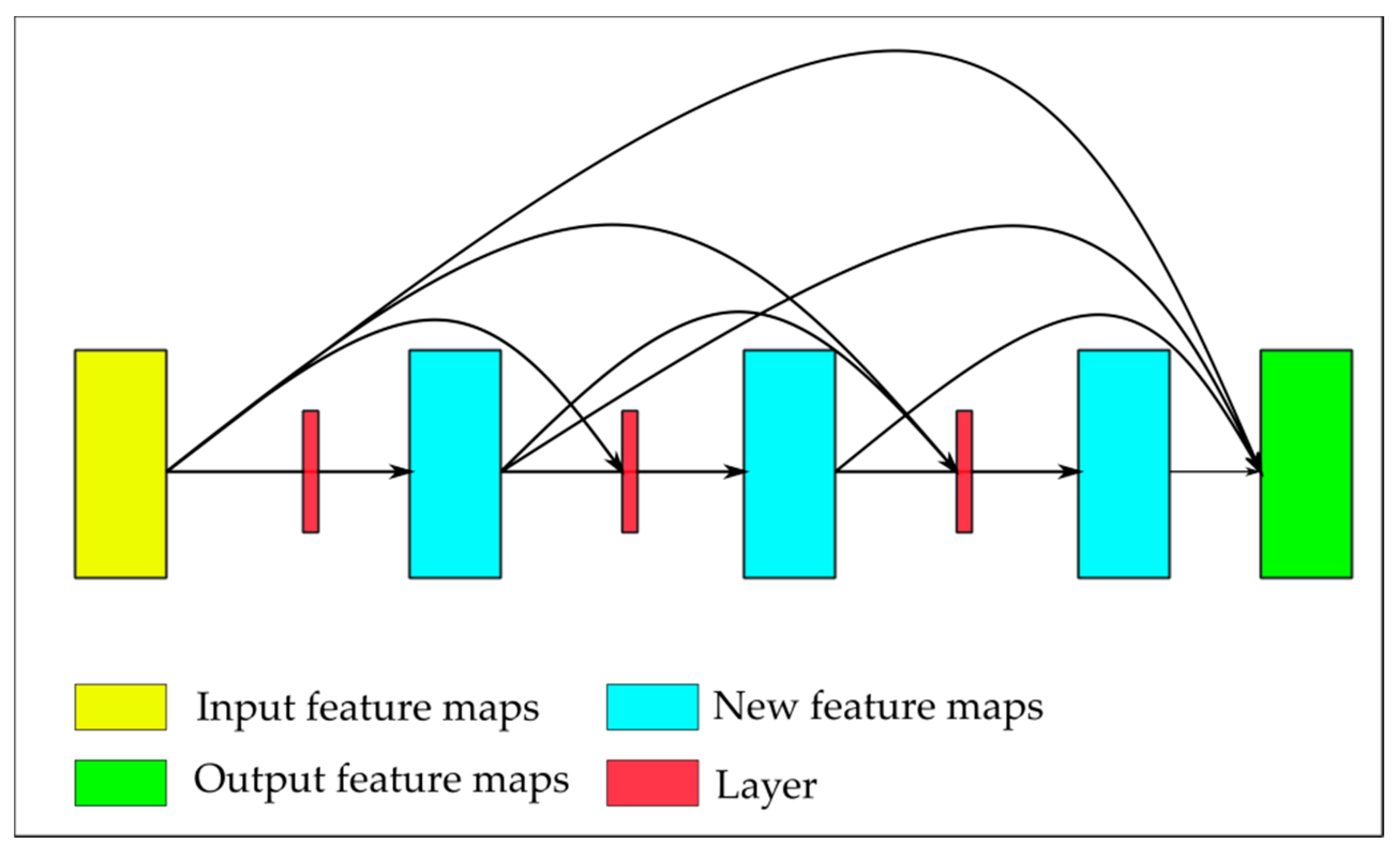
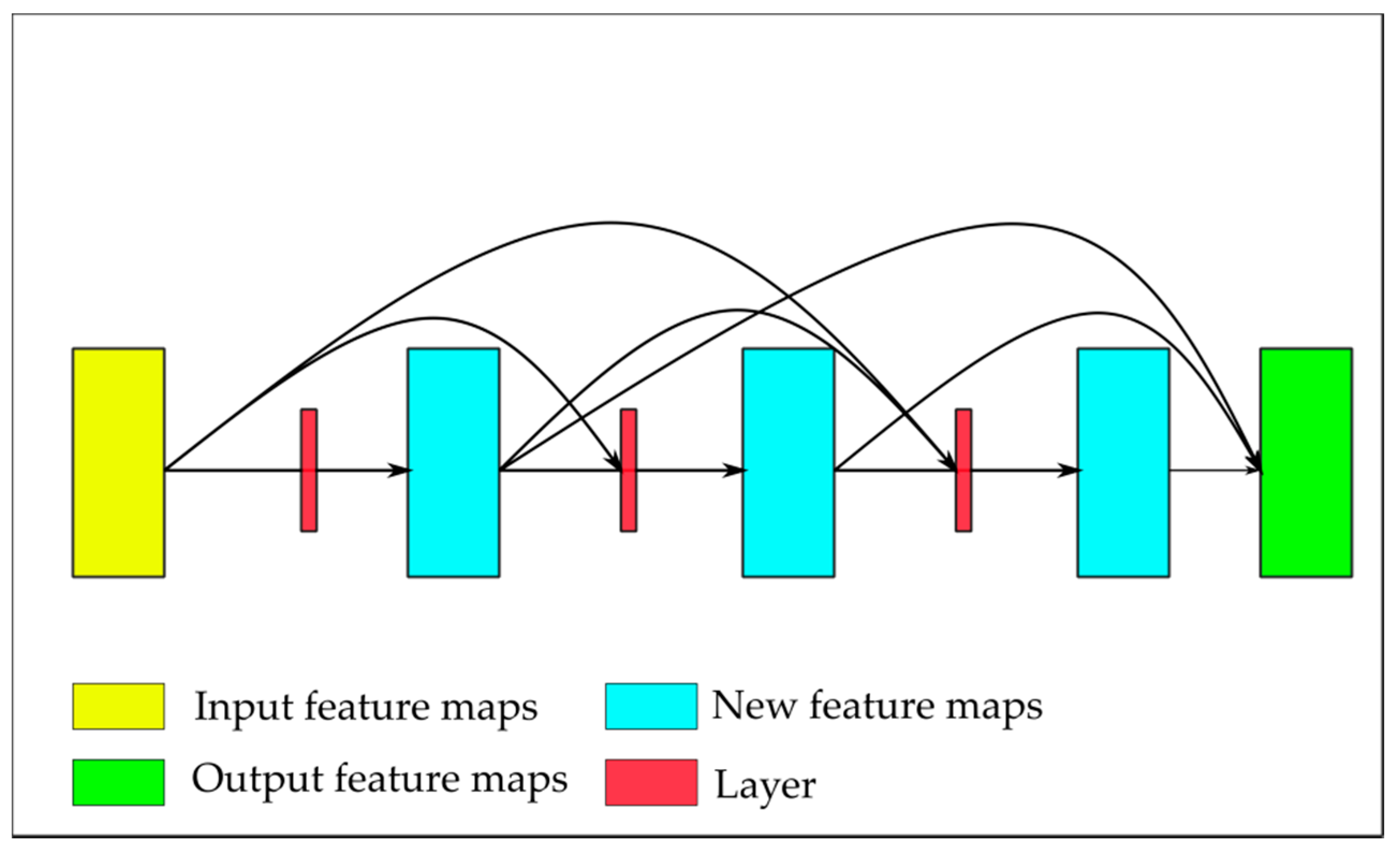
• We use fully convolutional DenseNets to extract buildings from remote sensing imagery. We demonstrate that dense connectivity improves the accuracy of common CNN models when extracting buildings from remote sensing imagery.
• We propose a full dense connectivity decoder that preserves the connections in all layers while reducing the required computation.
• We apply a compression approach to regulate and aggregate information from skip connections before entering the decoder.
• We supply a new CNN-based model called a multiple-feature reuse network (MFRN) for extracting buildings from remote sensing imagery that can make use of hierarchical image features.

The remainder of the paper is organized as follows. Related works on semantic segmentation methods in computer vision and remote sensing imagery are introduced in Section 2. In Section 3, we describe the details of our proposed method. Section 4 presents an experiment and an analysis of the results. The characteristics of our proposed MFRN are discussed in Section 5. Finally, Section 6 provides a conclusion.

2. Related Works

In this section, we describe previous approaches relevant to our proposed method.

2.1. CNNs

In recent years, convolutional neural networks [21] have become the most successful methods in computer vision and have achieved high accuracy. CNNs are composed of repeated connected convolutional layers that extract hierarchical image features [7]. The output of each convolutional layer is called a feature map, and each feature map forms the input of the next convolutional layer. The convolutional layer performs convolutional operations on the input feature maps using a small kernel (usually with a size of 3 × 3 pixels). The size of the new generated feature maps is determined by the number of kernels. Typically, convolutional layers in CNNs are followed by a nonlinear layer and a pooling layer [7]. The rectified linear unit [22] is usually chosen as the nonlinear activation function applied to each value in the feature maps. The pooling layer reduces the width and length of the feature maps by one half. Hence, the pooling layers increase the receptive field of the subsequent convolutional layers’ kernels, allowing them to capture larger image features. Moreover, the pooling layers also reduce the computation required when using large images. There are also many methods for feature extraction in remote sensing data, such as the spectral-spatial methods [23], object-based method [24], and hierarchical clustering [25]; however, CNN-based methods have an advantage of training models to learn features from a large dataset without the need for prior criteria. In this paper, we focus on CNN-based methods. Before the FCN was proposed, the most common method using CNNs for pixel-level classification was the patch-based method, which classifies pixels by analyzing the region around each pixel. Several works have used this approach to extract man-made objects from remote sensing imagery [10,11,12]. However, this method is slow because redundancy occurs due to overlapping patches, and there is a trade-off between localization accuracy and the use of context [26]. In this paper, we build our model based on the fully convolutional network (FCN) which is a decoder and encoder architecture with skip connections.

2.2. Decoder and Encoder Architectures

CNNs originally trained for image classification can be transferred to dense prediction tasks such as semantic segmentation by transforming the fully connected layers at the end of the CNN into convolutional layers, enabling a classification network to output a heat map [9]. In this way, one can obtain a low-resolution segmentation map. Consequently, up-sampling operations are required to recover the resolution of the segmentation map. The encoder–decoder architecture is based on this strategy: the encoder extracts features from the input image, and the decoder produces a segmentation map from the feature maps output by the encoder. Typically, the encoder is a CNN structure composed of a stack of convolutional layers, non-linear layers and pooling layers, while the decoder is composed of convolutional layers, non-linear layers and up-sampling operations. The output of each convolutional layer in the encoder contains the features captured by kernels with differently sized receptive fields. The decoder enlarges the feature maps extracted by the encoder to produce a final segmentation map that has the same resolution as the input image. Many semantic segmentation methods have been based on this encoder–decoder architecture [9,26,27,28]. Similar methods have been widely used for man-made object extraction from remote sensing imagery [13,16,17,18,29,30].

2.3. Skip Connections

Using a decoder, one can obtain a coarse segmentation map by simply directly enlarging the feature map of the encoder to the original size; however, the result will be poor in detail. This occurs because the change of the feature maps’ resolution results in a loss of location information. There are two main approaches to avoid location information loss. One approach is to use dilated convolutions to increase the receptive field instead of using pooling layers [14]—a strategy that has been applied to remote sensing imagery [13,15]. However, the dilated convolutions strategy is computationally expensive. Instead, using pooling layers to reduce feature map resolution not only increases the receptive field of subsequent convolution kernels but also reduces the amount of computation required when processing large images. Models based on dilated convolution must perform convolutional operations on high-resolution feature maps through the entire network, which makes such models difficult to train.

The second approach is to use skip connections [9]. A skip connection directly connects a convolutional layer in the encoder and a corresponding layer in the decoder. This approach is based on the fact that the early layers in the encoder include rich pixel location information in the skip connections. Thus, fusing the feature maps of earlier layers with the discriminative feature maps up-sampled at the end of the encoder step can obviously refine the segmentation map. Therefore, the skip-connections approach is widely used in encoder–decoder models [9,26,31,32,33]. In the remote sensing field, many encoder–decoder models have employed skip connections to improve accuracy [16,17,18,34,35,36].

3. Method

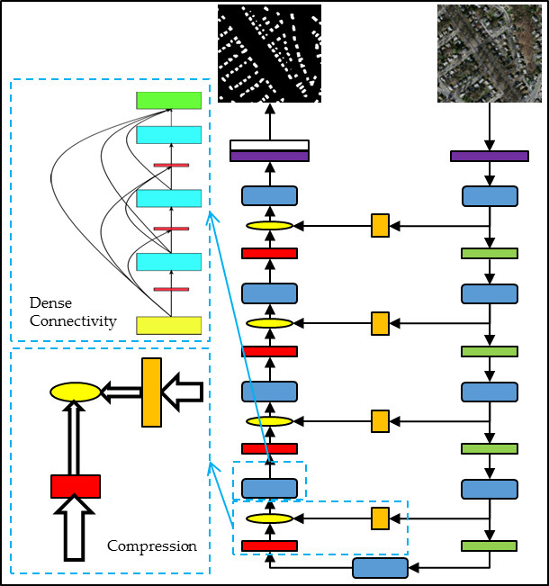
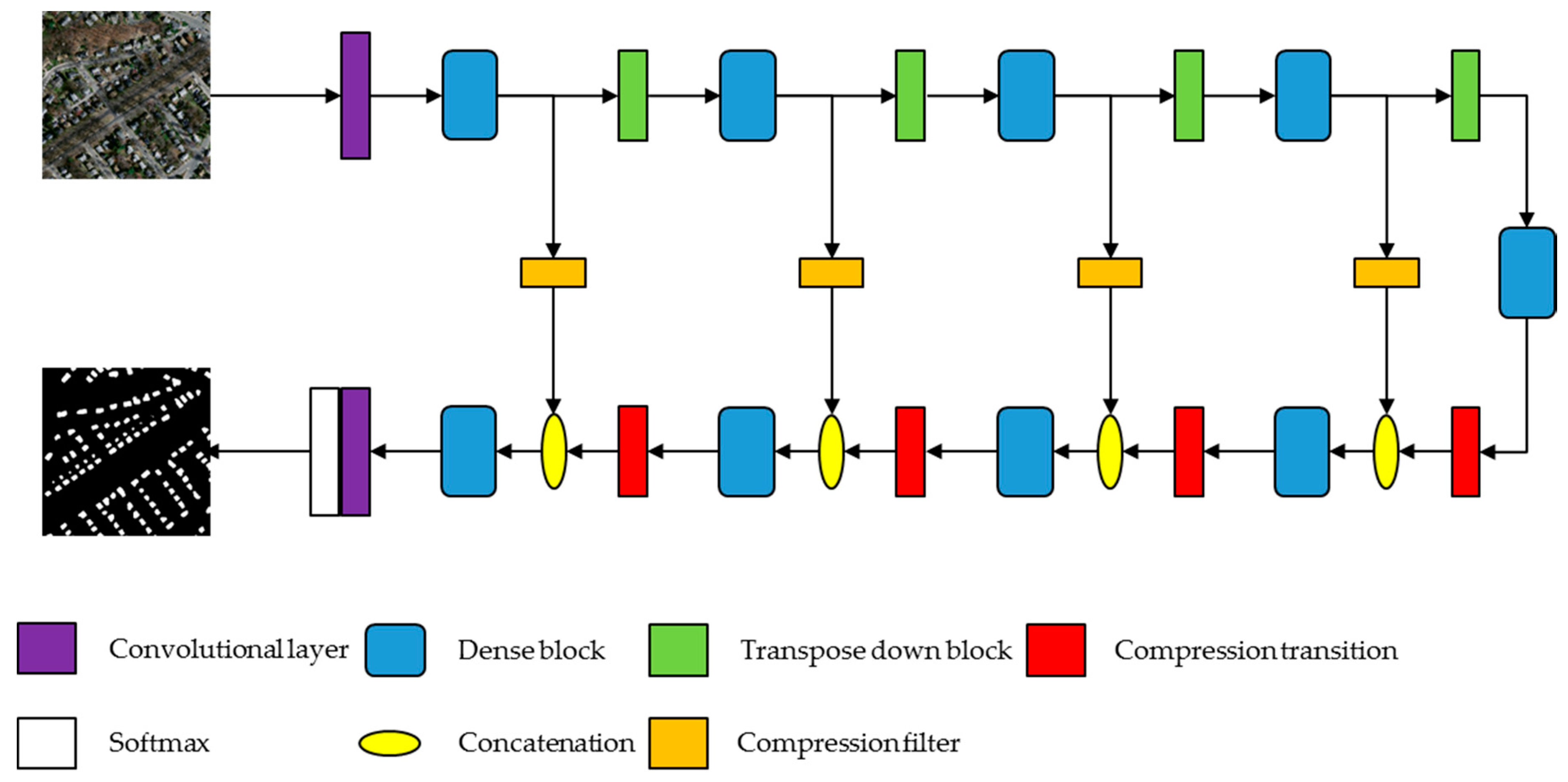
3.1. Overview of the Proposed Method

We propose a new encoder–decoder architecture that connects each layer with all the subsequent layers, allowing each layer to reuse features captured by earlier layers to perform building extraction from remote sensing imagery.

Figure 1 shows an overview of the proposed model. Inspired by DenseNets [20], the encoder was designed to extract features at multiple levels, while the decoder was designed to aggregate the multiple feature levels output by the different encoder layers. Both the encoder and decoder were built from dense blocks with dense connectivity to allow the multiple features to be reused and to reduce information loss through the network. Specifically, we propose a novel decoder that preserves the contributions of all layers to the final result and reduces the GPU memory demand. Moreover, we applied skip connection filters to balance the information that comes from the skip connections and the convolutional layers’ output.

In this section, we describe the major components of our proposed model, which include: (1) dense blocks; (2) compression transitions; and (3) skip connection filters.

3.2. Dense Block

Typically, convolutional networks are composed of repeated connected convolutional layers. Thus, a convolutional network with L layers has L connections. Each layer contains a non-linear transformation function $H_l$, where function $H_l$ usually consists of several operations such as convolutions, rectified linear units [22], pooling and dropout [37]. We use $x_l$ to denote the output of the $l^{th}$ layer. The traditional convolutional feed-forward networks connect the output of the layer as input to the layer, which gives rise to the following layer transition:

$$x_l=H_l\left(x_{l-1}\right).$$

(1)

To reduce the information loss in a deep convolutional network, DenseNets reuses information from previous layers through the idea of dense connectivity. In a DenseNet connectivity pattern, each layer is connected to all the subsequent layers of the same size. As a result, the $l^{th}$ layer receives the feature maps produced by all the preceding layers, $x_0,x_1,\dots .,x_{l-1}$, as input:

$$x_l=H_l\left(\left[x_0,x_1,\dots .,x_{l-1,}\right]\right)$$

(2)

where $\left[x_0,x_1,\dots .,x_{l-1}\right]$ denotes the concatenation of all the feature maps from all the preceding layers 0, …, L − 1. In DenseNets, function $H_l$ is defined as a function that comprises batch normalization [38], ReLU, convolution and dropout.

Dense connectivity resembles the skip connections of FCNs in that it merges different feature maps together; however, while each FCN skip connection connects one layer in the encoder with one layer in the decoder, dense connectivity repeatedly merges the feature maps output by all the previous layers in the network. This approach is highly conducive to making better use of the multiple features.

In our work, we use the term “dense block” to denote a set of convolutional layers connected using dense connectivity (see Figure 2). The first layer (red block) in a dense block produces k feature maps, where k is referred to as the growth rate. These k feature maps are concatenated with the input and transferred to the second layer. The second layer also outputs k feature maps, which are again concatenated with the input and the output of the previous layer. The third layer accepts all the previous feature maps and, again, outputs k feature maps. The final output of this dense block is a stack of feature maps that includes the input feature maps and each layer’s output feature maps. The layer composition details are listed in

Table 1. Layer composition in a dense block.

Layer in the Dense Block
BatchNormalization
ReLU
3 × 3 Convolution
Dropout

.

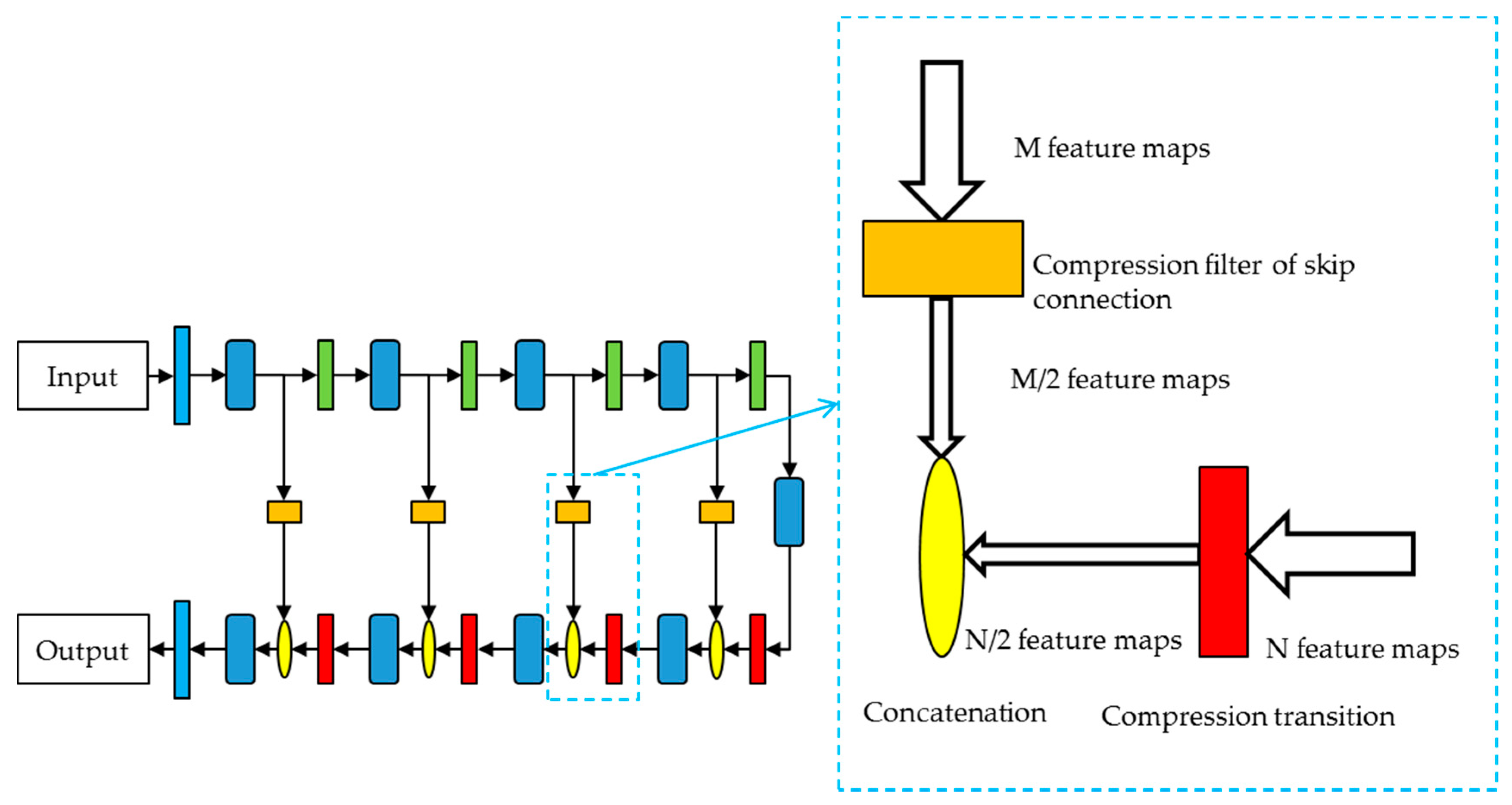
3.3. Decoder with Compression Transition

In our proposed method, the encoder has an architecture similar to that of DenseNets. However, that does not mean that a decoder with the same structure as the encoder will work well. As mentioned earlier, each dense block outputs both new feature maps produced by its layers and the input feature maps produced by the previous dense block. This results in a growth in the number of features through the network. Considering the increasing resolution of feature maps in the decoder and its concatenations with the feature maps of early layers through skip connections, the decoder would require enormous amounts of memory due to the convolution operation on the large number of high-resolution feature maps.

One solution to reduce the memory demand is to remove some connections in the decoder [19]. As Figure 3 shows, this approach does not concatenate the input of a dense block with its layers’ output in the decoder. Nevertheless, this approach runs counter to the DenseNets idea of preserving the direct contributions of all layers to the final classification.

To reduce the memory demand without breaking the dense connectivity, we use a transposed convolution layer [9] as a compression transition after each dense block in the decoder. The compression transition receives all the feature maps produced by the previous dense block and halves the number of feature maps. For this purpose, we allow a transposed convolutional layer following each dense block in the decoder to generate $q\times m$ output feature maps, where m is the number of feature maps produced by the dense block, and 0 < q ≤ 1 is the compression factor. When q = 1, the number of feature maps remains unchanged. This approach is illustrated in Figure 4. The red block received N feature maps and output N/2 new feature maps. We set q = 0.5 as the compression factor in our experiments. Every step in the decoder consists of a dense block followed by a 2 × 2 transposed convolution with a stride of 2 × 2 and a concatenation with the corresponding feature maps from the encoder. The main idea is that we allow the transposed convolution to reduce the number of feature maps while increasing the resolution of feature maps at each step to avoid a large number of high-resolution feature maps in the late stage of the decoder path.

3.4. Skip Connection Filter

Although compressing the transposed convolutional layer is effective in reducing the number of feature maps, another problem exists. The authors of [31,32] noted that the high-resolution feature maps with rich spatial location information in the early layers are less discriminative; consequently, directly passing them to the decoder through skip connections may add ambiguity to the final result. Thus, since we use a compression transition following each dense block in the decoder, the subsequent dense block receives a concatenation, including all the less discriminative feature maps from the skip connection and a compressed number of high discriminative feature maps generated by the previous block. To prevent the “where” location information from weakening the “what” classification information, we propose a skip connection filter, which is an additional convolutional layer with 3 × 3 convolution kernels that compress the feature maps from the skip connections. This additional convolutional layer receives all the feature maps from a dense block in the encoder and outputs new feature maps with half the number of the input. As a result, both feature maps from the skip connections and the previous dense block are compressed before passing to the next dense block in the decoder. In addition, this skip connection filter further aggregates the feature maps from different layers of the corresponding dense block in the encoder. The skip connection filter is illustrated in Figure 4. The skip compression filter compresses the M feature maps coming from the encoder through the skip connection by one half, and the newly generated $M/2$ feature maps are passed to the decoder. In our experiment, all connection filters and compression transitions share the same compression factor. Moreover, we conducted experiments to compare the performance of our models using different compression factors.

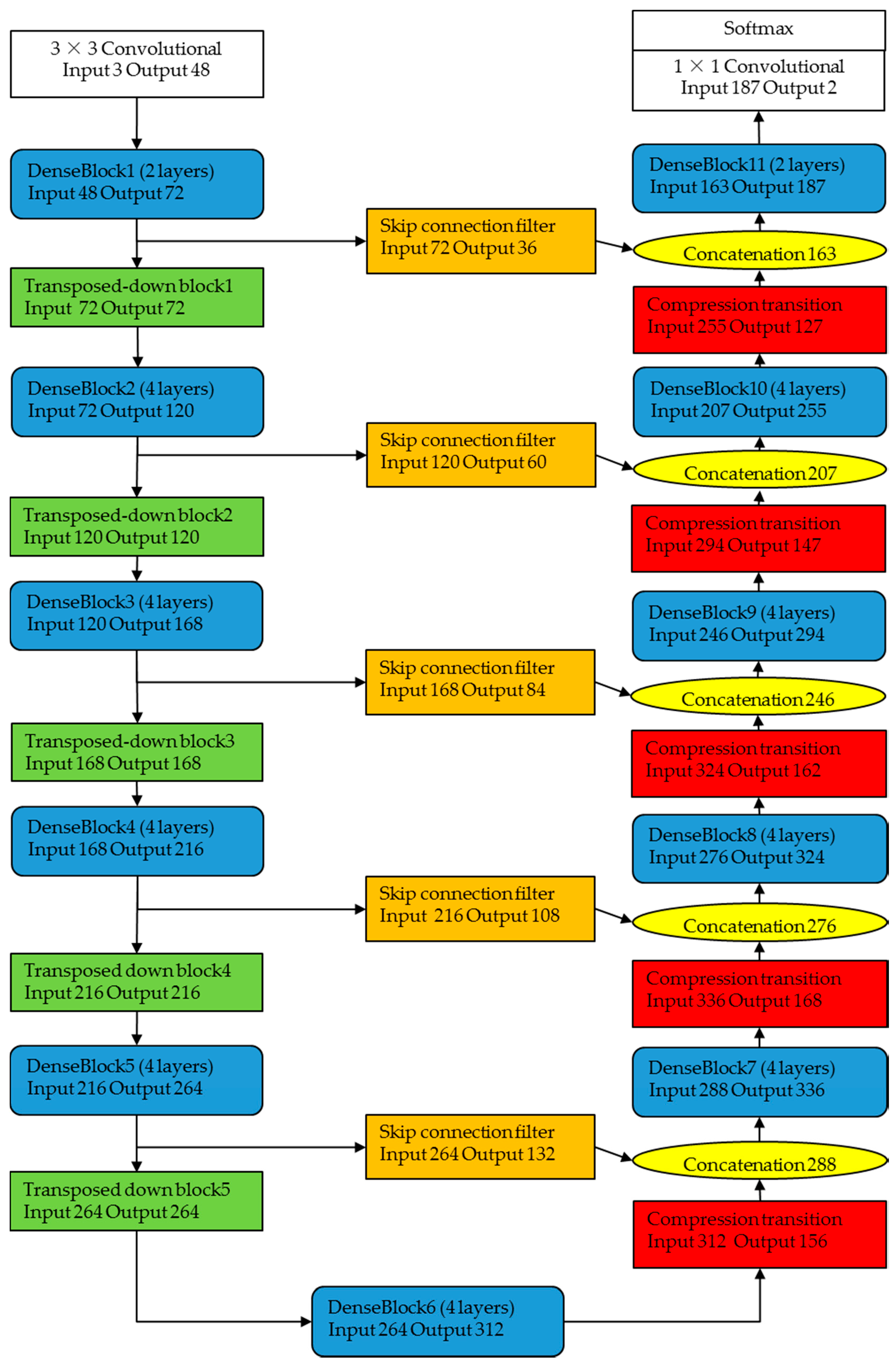
3.5. Implementation Details

The MFRN used in our experiment has 11 dense blocks that include 56 convolutional layers in the encoder and decoder. The structure of the proposed method is detailed in Figure 5. Before entering the first dense block, a convolutional layer with 48 3 × 3 kernels is applied to generate the initial feature maps. For all convolutional layers with 3 × 3 kernels, the outputs are zero-padded by one pixel to maintain a consistent feature map size for concatenations with other feature maps. In the encoder, we use a transpose-down block that includes a convolutional layer and a 2 × 2 average pooling layer. Conversely, in the decoder, we use a transpose-up block that includes a 2 × 2 transposed convolutional layer. At the end of the network, a convolutional layer with a softmax classifier [39] is used to output the final prediction. The number of feature maps generated by each convolutional layer in the dense block is set as 12. It can be found that the number of feature maps is compressed by skip connection filters and compression transitions repeatedly in the decoder.

3.6. Post Processing

CNNs can typically address only a small patch of the input image at any given time (e.g., 224 × 224 due to GPU memory limitations). To obtain a segmentation map that has the same size as the original high-resolution remote sensing imagery, the segmented patches must be combined. However, simply cropping patches from the imagery one after the other for building extraction and combining them will result in obvious stitching traces. These traces occur because the margins of the patches cropped from the remote sensing imagery usually include limited context information. Moreover, the padding operations add noise to the feature maps. These factors could result in misclassifications at patch margins. To solve this problem, we cropped patches from the imagery using a sliding cutting approach and use only the internal region of each segmented patch for the final combination. The margin of each patch with the potential for misclassification is covered by overlapping the sliding cutting operation. In our experiments, we used an overlap of 80 pixels. This approach is displayed in Figure 6. Each time a patch is segmented by the model, we keep only the interior yellow region, and the margin is abandoned. The overlapping part of two patches in the purple rectangle covers the margin in orange that we do not want, and the yellow region of two patches can then be combined coherently.

4. Experiment

4.1. Datasets

We evaluated our method on the Massachusetts Building Dataset created by Mnih [12]. The Massachusetts Building Dataset is a large remote sensing dataset composed of 1 m spatial resolution RGB aerial imagery at a resolution of 1500 × 1500 pixels. The dataset contains 151 images totally and was randomly split into a training set of 137 images, a test set of 10 images and a validation set of 4 images. We cropped the images into 320 × 320 patches and added images rotated by 90 degrees for data augmentation. In total, the training set includes 12,020 patches. We followed [20] and divided the pixel values by 255 so that they are in the [0,1] range. We used the test set for evaluation.

4.2. Training

In these experiments, we implemented all the models using the Keras framework [40]. We initialized our models using glorot_uniform [41] and trained them using Adam [42] with the initial learning rate of 0.001 chosen in [42]. Adam is a simple and computationally efficient adaptive method that computes individual adaptive learning rates for different parameters from estimates of first and second moments of the gradient. With the advantages of Adam, we could train all the models in our experiments efficiently without tuning the parameters, including the learning rate, the amount of momentum, and the type and amount of weight decay. All models were trained on the same dataset with the same augmentation. We trained all models for 50 epochs using a mini-batch size of 4 to make full use of the GPU memory. The dropout rate for all dropout layers was set to 0.2, which was chosen in [20]; the number of the growth rate was set to 12 following [19]; and the compression factor for skip connection filters and compression transition was set to 0.5. We also conducted experiments using different compression factors to analyze the compression factor’s influence on the result. The GPU used to train all the models was a GTX 1080 Ti.

4.3. Metrics

As the metrics to assess our method’s ability to classify buildings, we used overall accuracy, which is the percentage of correctly classified pixels, and the F1-score (F1). The F1-score is defined as follows:

$$\mathrm{F}1=\frac{2\times \mathrm{Precision}\times \mathrm{Recall}}{\mathrm{Precision}+\mathrm{Recall}},\mathrm{Precision}=\frac{\mathrm{TP}+\mathrm{TN}}{\mathrm{TP}+\mathrm{FP}+\mathrm{FN}+\mathrm{TN}},\mathrm{Recall}=\frac{\mathrm{TP}}{\mathrm{TP}+\mathrm{FN}}$$

(3)

where TP denotes true positive values, TN denotes true negative values, FP denotes false positive values, and FN denotes false negative values.

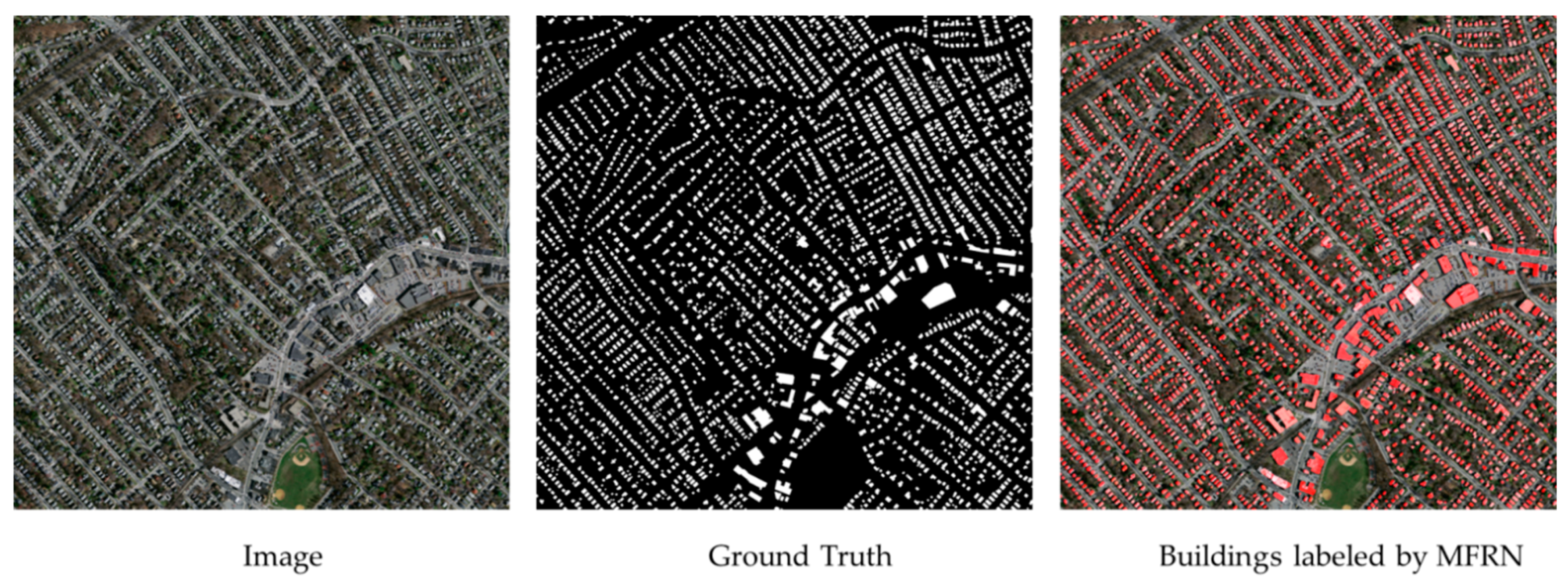
4.4. Results and Analysis

We implemented FCN-8s models following [9], a U-Net with 32, 64, 128, 256 and 512 channels in each stage following [26], and a 56-layer fully convolutional DenseNet following [19]. For our MFRN, the compression factor was set to 0.5. Considering that the compression in the decoder and skip connections is the most important modification we made, we kept the parameters chosen by the fully convolutional DenseNets as much as possible and compared the performance of our method using different compression factors. Hence, we conducted experiments using a compression factor of 0.4 and 0.3 to make comparisons. Next, we trained an MFRN with 56 layers and an MFRN with no skip connection filters (to do this, we had to remove 2 layers in the 2nd and 10th dense blocks due to GPU memory limitations). We also trained a “short version” MFRN with only 47 layers to evaluate our method’s performances with different network depths. Some segmented patches are shown in Figure 7. In

Table 2. Comparison results of different models.

Metric	Parameters	Time for Each Batch	Overall Accuracy	F1
FCN8	134.27 million	851 ms	93.27%	81.38%
U-Net	7.7 million	790 ms	93.63%	81.93%
FC-DenseNet56	3.49 million	775 ms	93.84%	83.54%
MFRN with compression factor 0.3	1.57 million	752 ms	93.88%	82.38%
MFRN with compression factor 0.4	2.07 million	746 ms	94.36%	84.45%
MFRN with compression factor 0.5	2.81 million	792 ms	94.51%	85.01%
MFRN with no filters	2.70 million	780 ms	94.20%	83.29%
Short MFRN with compression factor 0.5	1.87 million	785 ms	93.68%	82.06%

, we report the results of the trained models, the number of parameters and the time cost for training each 4-image patch, and Figure 8 illustrates the final images with buildings labeled by the MFRN.

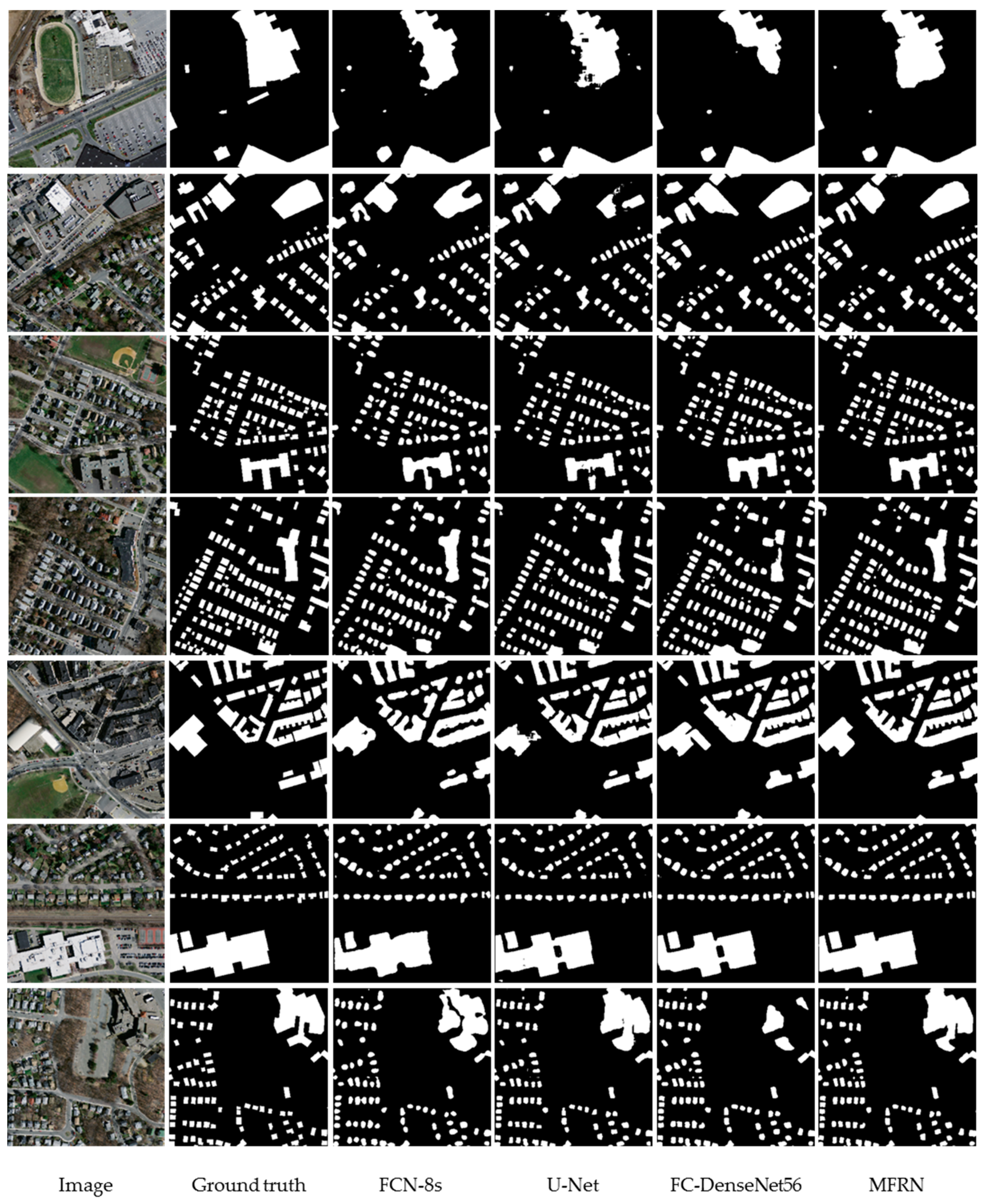
4.4.1. Comparison between MFRN and Other Models

The MFRN outperformed the common one-by-one connected CNN model structure FCN8 and U-Net by 3.63% and 3.08% in the F1 score, respectively. Meanwhile, our 56-layer MFRN with a compression factor of 0.5 exceeded the FC-DenseNet56 by 1.47% in the F1 score. In addition, our MFRN has a much smaller model size (parameter number) than the compared methods. Figure 7 shows that U-Net achieves a better performance than FCN-8s when extracting crowded small buildings, but its performance is less complete at extracting large buildings. FC-DenseNet56 has a more balanced performance in extracting both crowded small buildings and large buildings, but obvious misclassifications exist. Our MFRN produced a more refined and complete extraction and achieved a higher score for both crowded small buildings and large buildings. This finding suggests that the dense connectivity can significantly improve the performance of an FCN-based method. Models can achieve a better performance when extracting both small and crowded buildings and large buildings due to the reuse of multiple features in dense connectivity. Moreover, the experiments show that our method can make good use of dense connectivity while compressing the model size significantly.

4.4.2. Comparison between MFRNs with Different Parameters and Structures

The experiment of MFRNs with different compression factors shows that there is a trend that MFRN achieves a higher performance with the compression factors. We attribute this performance primarily to the growth in model capacity. We further analyzed it using SPSS V.17 (SPSS Inc., Chicago, IL, USA). The compression factor and the models’ performance on the test sets in the F1-score were analyzed by one-way ANOVA and least-significant difference tests. A probability level of p < 0.05 was set as the threshold of statistical significance. The analyses are shown in

Table 3. Descriptive statistics.

					95% Confidence Interval for Mean
	N	Mean	Std. Deviation	Std. Error	Lower Bound	Upper Bound
0.3	10	0.821610	0.0093475	0.0029560	0.814923	0.828297
0.4	10	0.838430	0.0110515	0.0034948	0.830524	0.846336
0.5	10	0.842170	0.0138517	0.0043803	0.832261	0.852079
Total	30	0.834070	0.0143972	0.0026286	0.828694	0.839446

,

Table 4. ANOVA.

	Sum of Squares	df	Mean Square	F	sig
Between Groups	0.002	2	0.001	8.964	0.001
Within Groups	0.004	27	0.000
Total	0.006	29

and

Table 5. Multiple comparisons.

(I) Compression Factor	(J) Compression Factor				95% Confidence Interval
		Mean Difference (I-J)	Std. Error	Sig.	Lower Bound	Upper Bound
0.3	0.4	−0.0168200 *	0.0051729	0.003	−0.027434	−0.006206
	0.5	−0.0205600 *	0.0051729	0.000	−0.031174	−0.009946
0.4	0.3	0.0168200 *	0.0051729	0.003	0.006206	0.027434
	0.5	−0.0037400	0.0051729	0.476	−0.014354	0.006874
0.5	0.3	0.0205600 *	0.0051729	0.000	0.009946	0.031174
	0.4	0.0037400	0.0051729	0.476	−0.006874	0.014354

* The mean difference is significant at the 0.05 level.

.

The compression factor significantly influenced the performance of MFRN (one-way ANOVA, p < 0.05). The group with compression factors of 0.4 and 0.5 showed a significant increase in the result compared with the group with the compression factor of 0.3. In addition, there was no significant increase in the result of the group with the compression factor of 0.5 compared to group with the compression factor of 0.4. This suggests that the compression transition and skip connection filters can help to make use of dense connectivity in building FCN models while controlling the model size to make full use of the GPU memory. When we compress the number of feature maps too much, the model capacity will be too small to achieve a high performance. However, increasing the compression factor from 0.4 to 0.5 did not obtain a significant increase in performance while increasing the model capacity and GPU memory demand. Therefore, we did not further increase the compression factor to conduct experiments.

The performance differences between the MFRN and the MFRN without compression filters in the skip connections showed that the skip connection filters help improve the model’s accuracy. When we implemented an MFRN without the compression filters, the GPU memory demand increased, and we had to remove two layers in the 2nd and 10th dense blocks, which suggests that adding the compression filter to the skip connections also effectively reduces the number of computations required. In addition, our MFRN showed a possible performance improvement as the depth increased.

5. Discussion

5.1. Model Size

As stated above, the DenseNets architecture is more compact than that of most other CNNs due to its feature reuse [20]. Consequently, MFRN and FC-DenseNet56 (which are both based on dense connectivity) have many fewer parameters than do the compared FCN-8s and U-Net models. For example, our proposed 56-layer MFRN has 2.8 million trainable parameters while the FCN-8s has 134 million trainable parameters. This is because most existing methods based on encoder–decoder structures such as FCN-8 and U-Net generally use a growing number of kernels in the convolutional layers to extract increasingly high-level features (e.g., 256, 512). In contrast, dense connectivity uses a small number called the growth rate (e.g., 12 or 16), and each layer outputs the same number of feature maps. This strategy enables a narrow and parameter-efficient model. To reduce the GPU memory demand without removing the connections between some layers, we apply compression in the transfer layer to control the number of feature maps, which further improves network compactness.

5.2. Reuse of Multiple Features

In common encoder–decoder structures, a merge of the feature maps from different layers occurs only between a layer in the decoder and the corresponding layer in the encoder through a skip connection. The MFRN has basic encoder/decoder sections that resemble U-Net but are characterized by dense connectivity between the different layers. Therefore, the multiple image features captured by each layer are reused by each subsequent layer. Compared with the two-layers fusion approach commonly used in encoder–decoder structures, MFRN strongly encourages the use of multiple image features captured by the different layers.

We found that, when the skip connections transferred large numbers of feature maps from the encoder (more than the number of discriminative feature maps generated by the dense block in the decoder), the classification accuracy is influenced. The compression mechanisms in both the skip connections and the decoder in our model help to balance the information from the skip connections with the information from the dense blocks in the decoder. Moreover, our approach also reduces the GPU memory requirements in the decoder.

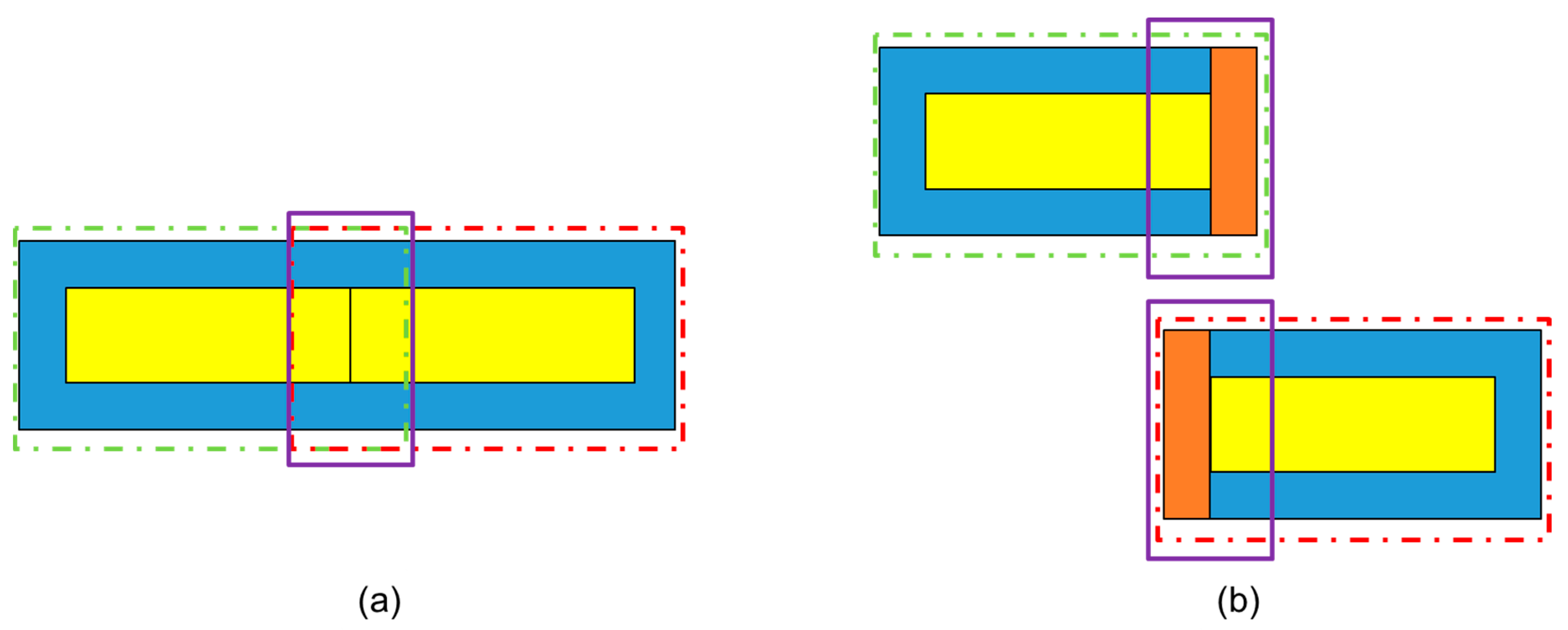
5.3. Overlapped Sliding Cutting

We applied an overlapped sliding cutting approach to avoid the potential for misclassifications in patch margins. Using this approach, the margins of the segmented patches are covered by the overlap between patches. We found that this strategy effectively reduces the stitching traces. It is worth noting that the size of the overlap between patches also influences the accuracy slightly. In our experiments, we found that an overlap of 80 pixels produces a better result. However, this number may not be the best choice for other datasets due to differences in the appearances of the extraction targets. When applying this approach to a new dataset, further exploration of the optimal overlap size is necessary.

6. Conclusions

In this paper, we demonstrate how dense connectivity can improve the accuracy of common encoder–decoder architectures when extracting buildings from remote sensing imagery. These improvements occur because each convolutional layer in a dense block has direct access to multiple levels of image features captured by previous layers. Moreover, this is a more parameter-efficient approach.

We designed a new decoder with compression layers to preserve the contributions of all layers to the final result while reducing the GPU memory requirements. We also introduced compression layers to regulate and aggregate the spatial location information from the skip connections to preserve the classification information in the decoder. Finally, we proposed a new encoder–decoder structure (MFRN) to extract buildings from remote sensing imagery.

In our experiments, our method achieved a higher accuracy on a large real-world remote sensing dataset than did the compared common encoder–decoder structure and fully convolutional DenseNets. It is worth noting that our experiment used only a single consumer-level GPU to train a 56-layer network. It is possible that a deeper MFRN with additional hyperparameter exploration could improve the performance. Nevertheless, our method achieved a high-accuracy result without pre-trained weights (94.5% overall accuracy). Further improvement may be achieved with a more appropriate initialization or by using pre-trained weights.

The training labels of the dataset in our experiment stem from common GIS data, which means there are many other training samples created by humans available to train CNN-based methods for building extraction tasks. With a larger number of training samples and further exploration of network depth and hyperparameters, we believe MFRN can facilitate many remote sensing imagery applications.

References

1. Ma, L.; Li, M.; Ma, X.; Cheng, L.; Du, P.; Liu, Y. A review of supervised object-based land-cover image classification. ISPRS J. Photogramm. Remote Sens. 2017, 130, 277–293. [Google Scholar] [CrossRef]
2. Tong, X.; Hong, Z.; Liu, S.; Zhang, X.; Xie, H.; Li, Z.; Yang, S.; Wang, W.; Bao, F. Building-damage detection using pre-and post-seismic high-resolution satellite stereo imagery: A case study of the May 2008 wenchuan earthquake. ISPRS J. Photogramm. Remote Sens. 2012, 68, 13–27. [Google Scholar] [CrossRef]
3. Moya, L.; Marval Perez, L.R.; Mas, E.; Adriano, B.; Koshimura, S.; Yamazaki, F. Novel unsupervised classification of collapsed buildings using satellite imagery, hazard scenarios and fragility functions. Remote Sens. 2018, 10, 296. [Google Scholar] [CrossRef]
4. Huang, X.; Wen, D.; Li, J.; Qin, R. Multi-level monitoring of subtle urban changes for the megacities of china using high-resolution multi-view satellite imagery. Remote Sens. Environ. 2017, 196, 56–75. [Google Scholar] [CrossRef]
5. Pang, S.; Hu, X.; Wang, Z.; Lu, Y. Object-based analysis of airborne lidar data for building change detection. Remote Sens. 2014, 6, 10733–10749. [Google Scholar] [CrossRef]
6. LeCun, Y.; Boser, B.E.; Denker, J.S.; Henderson, D.; Howard, R.E.; Hubbard, W.E.; Jackel, L.D. Handwritten digit recognition with a back-propagation network. In Advances in Neural Information Processing Systems; Touretzky, D.S., Mozer, M.C., Hasselmo, M.E., Eds.; MIT Press: Cambridge, MA, USA, 1990; pp. 396–404. [Google Scholar]
7. LeCun, Y.; Bottou, L.; Bengio, Y.; Haffner, P. Gradient-based learning applied to document recognition. Proc. IEEE 1998, 86, 2278–2324. [Google Scholar] [CrossRef] [Green Version]
8. Zeiler, M.D.; Fergus, R. Visualizing and understanding convolutional networks. In Proceedings of the ECCV 2014: Computer Vision–ECCV 2014 European Conference on Computer Vision, Zurich, Switzerland, 6–12 September 2014; Fleet, D., Pajdla, T., Schiele, B., Tuytelaars, T., Eds.; Springer: Berlin, Germany, 2014. [Google Scholar]
9. Long, J.; Shelhamer, E.; Darrell, T. Fully convolutional networks for semantic segmentation. In Proceedings of the IEEE Conference on Computer Vision and Pattern Recognition (CVPR), Boston, MA, USA, 8–10 June 2015; IEEE: Piscataway, NJ, USA, 2015. [Google Scholar]
10. Mnih, V.; Hinton, G.E. Learning to detect roads in high-resolution aerial images. In Proceedings of the European Conference on Computer Vision, Berlin, Germany, 5–11 September 2010; Daniilidis, K., Maragos, P., Paragios, N., Eds.; Springer: Berlin, Germany, 2010; pp. 210–223. [Google Scholar]
11. Alshehhi, R.; Marpu, P.R.; Woon, W.L.; Dalla Mura, M. Simultaneous extraction of roads and buildings in remote sensing imagery with convolutional neural networks. ISPRS J. Photogramm. Remote Sens. 2017, 130, 139–149. [Google Scholar] [CrossRef]
12. Mnih, V. Machine Learning for Aerial Image Labeling. Ph.D. Thesis, University of Toronto, Toronto, ON, Canada, 2013. [Google Scholar]
13. Sherrah, J. Fully convolutional networks for dense semantic labelling of high-resolution aerial imagery. arXiv, 2016. Available online: https://arxiv.org/abs/1606.02585 (accessed on 22 August 2018)arXiv:1606.02585.
14. Yu, F.; Koltun, V. Multi-scale context aggregation by dilated convolutions. arXiv, 2015. Available online: https://arxiv.org/abs/1511.07122 (accessed on 22 August 2018)arXiv:1511.07122.
15. Hamaguchi, R.; Fujita, A.; Nemoto, K.; Imaizumi, T.; Hikosaka, S. Effective use of dilated convolutions for segmenting small object instances in remote sensing imagery. arXiv, 2017. Available online: https://arxiv.org/abs/1709.00179 (accessed on 22 August 2018)arXiv:1709.00179.
16. Yuan, J. Automatic building extraction in aerial scenes using convolutional networks. arXiv, 2016. Available online: https://arxiv.org/abs/1602.06564 (accessed on 22 August 2018)arXiv:1602.06564.
17. Maggiori, E.; Tarabalka, Y.; Charpiat, G.; Alliez, P. High-resolution semantic labeling with convolutional neural networks. arXiv, 2016. Available online: https://arxiv.org/abs/1611.01962 (accessed on 22 August 2018)arXiv:1611.01962.
18. Maggiori, E.; Tarabalka, Y.; Charpiat, G.; Alliez, P. Convolutional neural networks for large-scale remote-sensing image classification. IEEE Trans. Geosci. Remote Sens. 2017, 55, 645–657. [Google Scholar] [CrossRef]
19. Jégou, S.; Drozdzal, M.; Vazquez, D.; Romero, A.; Bengio, Y. The one hundred layers tiramisu: Fully convolutional densenets for semantic segmentation. arXiv, 2016. Available online: https://arxiv.org/abs/1611.09326 (accessed on 22 August 2018)arXiv:1611.09326.
20. Huang, G.; Liu, Z.; Weinberger, K.Q.; van der Maaten, L. Densely connected convolutional networks. arXiv, 2016. Available online: https://arxiv.org/abs/1608.06993 (accessed on 22 August 2018)arXiv:1608.06993.
21. LeCun, Y.; Bengio, Y. Convolutional networks for images, speech, and time series. In The Handbook of Brain Theory and Neural Networks; Arbib, M.A., Ed.; MIT Press: Cambridge, MA, USA, 1998; pp. 255–258. ISBN 0-262-51102-9. [Google Scholar]
22. Glorot, X.; Bordes, A.; Bengio, Y. Deep sparse rectifier neural networks. In Proceedings of the Fourteenth International Conference on Artificial Intelligence and Statistics, Fort Lauderdale, FL, USA, 11–13 April 2011. [Google Scholar]
23. Tarabalka, Y.; Benediktsson, J.A.; Chanussot, J. Spectral–spatial classification of hyperspectral imagery based on partitional clustering techniques. IEEE Trans. Geosci. Remote Sens. 2009, 47, 2973–2987. [Google Scholar] [CrossRef]
24. Gao, Y.; Marpu, P.; Niemeyer, I.; Runfola, D.M.; Giner, N.M. Object-based classification with features extracted by a semi-automatic feature extraction algorithm—Seath. Geocarto Int. 2011, 26, 211–226. [Google Scholar] [CrossRef]
25. Senthilnath, J.; Kumar, D.; Benediktsson, J.A.; Zhang, X. A novel hierarchical clustering technique based on splitting and merging. Int. J. Image Data Fusion 2016, 7, 19–41. [Google Scholar] [CrossRef]
26. Ronneberger, O.; Fischer, P.; Brox, T. U-net: Convolutional networks for biomedical image segmentation. In Proceedings of the MICCAI 2015: Medical Image Computing and Computer-Assisted Intervention, Munich, Germany, 5–9 October 2015. [Google Scholar]
27. Badrinarayanan, V.; Kendall, A.; Cipolla, R. Segnet: A deep convolutional encoder-decoder architecture for image segmentation. arXiv, 2015. Available online: https://arxiv.org/abs/1511.00561 (accessed on 22 August 2018)arXiv:1511.00561. [CrossRef] [PubMed]
28. Noh, H.; Hong, S.; Han, B. Learning deconvolution network for semantic segmentation. In Proceedings of the 2015 IEEE International Conference on Computer Vision (ICCV), Santiago, Chile, 7–13 December 2015. [Google Scholar]
29. Audebert, N.; Le Saux, B.; Lefèvre, S. Beyond RGB: Very high resolution urban remote sensing with multimodal deep networks. ISPRS J. Photogramm. Remote Sens. 2017, 140, 20–32. [Google Scholar] [CrossRef]
30. Li, Y.; He, B.; Long, T.; Bai, X. Evaluation the performance of fully convolutional networks for building extraction compared with shallow models. In Proceedings of the 2017 IEEE International Geoscience and Remote Sensing Symposium (IGARSS), Fort Worth, TX, USA, 23–28 July 2017. [Google Scholar]
31. Lin, G.; Milan, A.; Shen, C.; Reid, I. Refinenet: Multi-path refinement networks for high-resolution semantic segmentation. In Proceedings of the IEEE Conference on Computer Vision and Pattern Recognition (CVPR), Honolulu, HI, USA, 21–26 July 2017. [Google Scholar]
32. Islam, M.A.; Rochan, M.; Bruce, N.D.; Wang, Y. Gated feedback refinement network for dense image labeling. In Proceedings of the 2017 IEEE Conference on Computer Vision and Pattern Recognition (CVPR), Honolulu, HI, USA, 21–26 July 2017. [Google Scholar]
33. Zhao, H.; Shi, J.; Qi, X.; Wang, X.; Jia, J. Pyramid scene parsing network. In Proceedings of the 2017 IEEE Conference on Computer Vision and Pattern Recognition (CVPR), Honolulu, HI, USA, 21–26 July 2017. [Google Scholar]
34. Xu, Y.; Wu, L.; Xie, Z.; Chen, Z. Building extraction in very high resolution remote sensing imagery using deep learning and guided filters. Remote Sens. 2018, 10, 144. [Google Scholar] [CrossRef]
35. Liu, Y.; Fan, B.; Wang, L.; Bai, J.; Xiang, S.; Pan, C. Semantic labeling in very high resolution images via a self-cascaded convolutional neural network. ISPRS J. Photogramm. Remote Sens. 2017. [Google Scholar] [CrossRef]
36. Wu, G.; Shao, X.; Guo, Z.; Chen, Q.; Yuan, W.; Shi, X.; Xu, Y.; Shibasaki, R. Automatic building segmentation of aerial imagery using multi-constraint fully convolutional networks. Remote Sens. 2018, 10, 407. [Google Scholar] [CrossRef]
37. Srivastava, N.; Hinton, G.; Krizhevsky, A.; Sutskever, I.; Salakhutdinov, R. Dropout: A simple way to prevent neural networks from overfitting. J. Mach. Learn. Res. 2014, 15, 1929–1958. [Google Scholar]
38. Ioffe, S.; Szegedy, C. Batch normalization: Accelerating deep network training by reducing internal covariate shift. arXiv, 2015. Available online: https://arxiv.org/abs/1502.03167 (accessed on 22 August 2018)arXiv:1502.03167.
39. Bridle, J.S. Probabilistic Interpretation of Feedforward Classification Network Outputs, with Relationships to Statistical Pattern Recognition; Springer: Berlin, Germany, 1990; pp. 227–236. ISBN 978-3-642-76153-9. [Google Scholar]
40. Chollet, F.; Keras. GitHub Repository. Available online: https://github.com/fchollet/keras (accessed on 22 August 2018).
41. Glorot, X.; Bengio, Y. Understanding the difficulty of training deep feedforward neural networks. In Proceedings of the Thirteenth International Conference on Artificial Intelligence and Statistics, Sardinia, Italy, 13–15 May 2010. [Google Scholar]
42. Kingma, D.P.; Ba, J. Adam: A method for stochastic optimization. arXiv, 2014. Available online: https://arxiv.org/abs/1412.6980 (accessed on 22 August 2018)arXiv:1412.6980.
Figure 1. An illustration of the architecture of the multiple-feature reuse network (MFRN). The MFRN is composed of an encoder and a decoder. An RGB image patch is input to the model. The purple blocks are convolutional layers. The white block following the final convolutional layer represents a softmax classifier. The blue blocks are dense blocks composed of a stack of densely connected convolutional layers. The green blocks represent a transpose-down block composed of pooling layers. The orange blocks represent the compression filters in the skip connections. The red blocks represent compression transitions composed of a transposed convolutional layer.
Remotesensing 10 01350 g001
Figure 2. A dense block with three convolutional layers. The red blocks represent a layer in a dense block.
Remotesensing 10 01350 g002
Figure 3. A dense block of the decoder in fully convolutional descent. The input of this dense block is not concatenated with the new feature maps in the final stage.
Remotesensing 10 01350 g003
Figure 4. An illustration of our proposed compression filter in skip connections and the compression transition in the decoder. The orange block represents the compression filter in the skip connection, and the red block refers to the compression transition in the decoder.
Remotesensing 10 01350 g004
Figure 5. Structural details of an MFRN with 56 convolutional layers. The number of input feature maps and output feature maps is listed in each block.
Remotesensing 10 01350 g005
Figure 6. (a) The figure shows two patches (green dotted line and red dotted line) that overlap. The internal yellow regions are coherent. The overlap of the two patches is covered in the purple rectangle. (b) The figure shows how the orange margin with the potential for misclassification is covered by the overlap of the two patches. The overlapped part of each patch in the purple rectangle contains the margin in orange. Since we keep only the yellow region of each segmented patch, the orange margin is abandoned.
Remotesensing 10 01350 g006
Figure 7. Segmented patches from FCN-8s, U-Net, fully convolutional DenseNets and MFRN. The white color in the segmented patches represents pixels belonging to buildings.
Remotesensing 10 01350 g007
Figure 8. An illustration of a 3 × 3 image, the corresponding building labels and the final processed image with buildings labeled by the MFRN.
Remotesensing 10 01350 g008