1. Introduction
A useful public health application of satellite remote sensing is to augment sparse monitoring networks and cover large time and space domains when modeling particulate matter for epidemiologic health studies [
1]. Recent refinements in remote sensing algorithms have resulted in higher resolution products such as the 1 × 1 km resolution Multi-Angle Implementation of Atmospheric Correction (MAIAC) retrieval algorithm estimating the Aerosol Optical Depth (AOD) as a measure of the density of light scattering particles in the atmospheric column [
2,
3]. The MAIAC product, derived for the Moderate Resolution Imaging Spectroradiometer (MODIS) instruments, like earlier lower spatial resolution AOD products (e.g., 10 km × 10 km Deep Blue and Dark Target retrieval algorithms), is a key predictor in leading statistical models estimating PM
2.5 at the ground level [
4,
5,
6].
Because of the challenge of estimating valid AOD measures over heterogeneous landscapes with varying remote sensing characteristics (e.g., view geometry at acquisition as measured by the relative azimuth), the resulting products can contain patterns that appear anomalous in visualizations, which suggests room for improvement. While previous work has compared the agreement of MAIAC with earlier MODIS 10 × 10 km AOD products and ground monitoring data in different regions and seasons by stratifying the dataset [
7], little work has been done to comprehensively understand and correct for measurement error in the MAIAC AOD product.
Quantifying and correcting measurement error in the MAIAC AOD product requires a comparison with a reliable validation dataset. The AErosol RObotic NETwork (AERONET) is a standardized ground-based remote sensing network for measuring aerosol optical depth with a cloud-screened and quality assured data record that is frequently used as a validation for satellite-based AOD products [
8].
In this application, we propose and compare three related ensemble machine-learning modeling approaches with a wide range of predictors related to data quality, context, and relevant spatial characteristics. These predictors are used to partially correct measurement error in satellite AOD versus data from AERONET stations across the region which are used as a validation. We demonstrate that this approach improves the MAIAC AOD product over the Northeastern USA. The resulting corrected AOD has a substantially improved correlation with ground-level PM2.5 and thus will be a key predictor in the next generation of satellite-hybrid PM2.5 air pollution models.
2. Materials and Methods
The study region was the Northeast and Mid-Atlantic USA including 13 states from Maine to Virginia. This region includes 629,729 centroids from a fixed grid that is approximately 1 × 1 km in resolution as produced for the MAIAC algorithm (
Figure 1). Satellite-derived AOD products from the MAIAC algorithm for both MODIS instruments on the Terra and Aqua satellites were obtained from NASA (version downloaded 16 October 2016). These data include AOD estimates as well as auxiliary variables such as uncertainty estimates, relative azimuth, and additional QC flags such as cloud adjacency masks (full variable list in results). The AOD data were collected from 24 February 2000 to 6 August 2016 and from 4 July 2002 to 31 August 2016 for Terra and Aqua, respectively. The MAIAC dataset is organized by orbit, with the number of acquisitions per satellite per day ranging from 1 to 3; the percentage of days with 2 acquisitions was equal to 78.1% for Terra (with local average overpass times of 9:52 a.m. and 11:31 a.m.) and 82.8% for Aqua (with local average overpass times of 11:51 a.m. and 1:29 p.m.). For those centroids with more than one value of AOD per day (coming from different acquisition times on the same day), making up almost 10% of the data; we kept the record with the lowest AOD uncertainty estimate from the MAIAC dataset.
All global Aerosol Optical Thickness (AOT—a synonymous term for AOD used by AERONET) measurements from AERONET sun photometers were downloaded from
https://aeronet.gsfc.nasa.gov/ (accessed 29 March 2017; Level 2.0, cloud-screened and quality-assured data; Version 2.0 Direct Sun Algorithm) and subset to the 79 AERONET stations in the study region (Maine to Virginia) with available data between 2000 and 2015 (
Figure 1). AERONET measures were joined to the Aqua or Terra derived MAIAC AOD, when available, from the fixed grid cell centroid closest to the AERONET location, using the AERONET measure closest in time to the satellite overpass (within 60 min).
Our outcome of interest was the difference between AOD and AOT (calculated as AOD-AOT); a residual that approximates the satellite product measurement error. We selected this as our parameter for three reasons: (1) the difference has an easier interpretation because our goal in modeling measurement error was to minimize the difference from the reference AOT; (2) the difference had an approximately normal distribution; and (3) because some ensemble modeling methods resample subsets of covariates, estimating AOT without first subtracting from AOD would lead to regression trees within the ensemble which do not include the AOD as a predictor.
Our modeling approach to estimate measurement error used a set of 52 total predictor variables. These included quality control features that are part of the MAIAC dataset (e.g., relative azimuth at acquisition and the MAIAC algorithm’s own AOD uncertainty estimate), GIS-derived land use and meteorologic covariates (e.g., nearest air temperature from the NOAA reanalysis and proportion of forest within 1 km from the National Land Cover Dataset [
9]), and spatially derived covariates engineered to capture characteristics of the data that were observed in visualizations and assigned to each centroid (e.g., number of non-missing AOD centroids within moving windows, difference of AOD from the mean within moving windows of varying edge lengths, and clump size of the number of contiguous non-missing AOD measures within a day). A detailed definition of the model equation including the 52 predictor variables, data sources, and their derivation are included in
Appendix A.
In this analysis we trained ensemble machine-learning methods for regression that operate by constructing a multitude of decision trees in a training set and using them to make predictions on a withheld test set. Specifically, we fit three machine-learning algorithms: Random Forest (RF) and two implementations of Gradient Boosting (GB) models. RF uses an ensemble of unpruned decision trees, each grown using a bootstrap sample of the training data, and randomly selected subsets of predictor variables as candidates for splitting tree nodes. The RF prediction for a new observation is the average of the output over all trees. Unlike RF that trains each tree independently, GB grows each tree on the residuals of the previous tree. This means that at each particular iteration, a new weak, base-learner model is trained with respect to the error of the whole ensemble learnt so far. Prediction is accomplished by weighting the ensemble outputs of all the regression trees.
We implemented RF using the
randomForest R package [
10]. Hyper-parameters were set to use 10,000 trees (ntrees) and to subsample ⅓ of the covariates in each tree (mtry). GB was implemented using two different R functions:
gbm (Generalized Boosted regression Models) and
xgboost (eXtreme Gradient Boosting) from the
gbm and
xgboost packages, respectively [
11,
12]. Although both GBM and XGBoost follow the principle of gradient boosting, XGBoost has some additional changes to improve predictive performance that makes it more of a hybrid of the GB and RF approaches [
13]. Specifically, XGBoost uses a more regularized model formalization to control for overfitting, and can also use a random subset of predictor variables at each node like in RF. Hyper-parameters for the GBM were set to use 10,000 trees (n.trees), allow up to 6 splits per tree (interaction.depth) and a learning rate of 0.002 (shrinkage), all selected based on previous tuning experience. For XGBoost, we also applied 5-fold cross-validation to the training set to tune the hyper-parameters of the model. Root Mean Square Error (RMSE) was used to select the optimal model hyper-parameters using the smallest mean value across the 5 folds. The final hyper-parameters for XGBoost for Aqua were 10,000 trees (ntree), allowing up to 5 splits per tree (max_depth), a learning rate of 0.01 (eta), using all features in each tree (colsample_bytree), and using half of the data in each tree (subsample). For Terra the hyper-parameters were the same except for allowing up to 6 splits per tree (max_depth) and subsampling only ⅓ of the covariates in each tree (colsample_bytree). In order to train and validate the performance of these three methods, we split the two datasets (for Terra and Aqua satellites) into training and testing sets. Because the relationship between AOD and ground conditions varies daily [
4], the testing sets were created by withholding all observations from randomly selected days across the study period such that the number of withheld testing observations were 15% of the entire dataset. Root Mean Square Prediction Error (RMSPE) of the testing set was used to assess and compare the performance of the three approaches for each satellite.
While predictors can have complex relationships in ensemble models, their contribution can be summarized with variable importance measures to quantify and partial dependence plots to visualize the way that predictions (in our case, measurement error) depends on covariates. Variable importance for the XGBoost model was quantified using the
xgb.importance function from the
xgboost R package that quantifies how splitting on each feature improves the purity of each node, which in regression tree models is the maximum likelihood estimator of the variance within the node. R functions for permutation testing were used to assess variable importance for both RF and GBM approaches. Both these methods randomly permute each predictor one variable at a time and compute the associated reduction in predictive performance: the higher the reduction, the more important the variable is in predicting the outcome. The only difference in these two functions is that, while GBM permutes the entire training dataset, RF uses only the out-of-bag observations. We also used the R function
max.subtree from the
randomForestSRC package [
14] to compute the first order depth of each variable using RF models—this represents the average number of splits within a tree between the root node and the first split on that variable. The smaller the first order depth the greater the impact of that variable on prediction. For visualization, partial dependency plots show the effect of a predictor variable on the target outcome, after accounting for the average effects of the other predictors—partialling them out.
We also tried fitting XGBoost using just the top 10 or top 20 most important predictors from the XGBoost model to assess the loss of information when using a more parsimonious feature set. In both cases, 5-fold cross-validation was again used on the training set to tune the parameters of the more parsimonious models before assessment on the testing set.
We implemented two methods to estimate the predictive uncertainty in our measurement error model: bootstrapping the ensemble learner (resampling with replacement and refitting the entire model multiple times), and running the Infinitesimal Jackknife (IJ) which has been developed for Random Forest models [
15,
16].
In previous work, we have demonstrated that AOD is the best single predictor for models to estimate PM
2.5 at the ground level, although the complex relationship is improved with daily calibrations [
4,
17,
18]. To demonstrate that the measurement error correction provided by our approach will help with the subsequent modeling of ground-level air pollution, we also compared the raw and corrected values of AOD with PM
2.5 measurements from all available monitors within the study region based on the EPA and IMPROVE monitoring networks [
4]. The AOD and PM
2.5 were compared with the Pearson correlation coefficient using non-missing AOD from the closest grid centroid (within 1 km of the monitoring station) and the daily average PM
2.5 concentrations. We remove one monitor (420030064, near Pittsburgh PA) due to aberrant values likely related to the proximity of large industrial facilities, including the Clairton Coke Works. This station is located in the Monongahela river valley across from and <3 km to the Clairton Coke Works, the largest coke manufacturing plant baking coal for steelmaking in the United States.
The resulting dataset included 362 and 381 PM
2.5 monitors with 105,798 and 131,788 daily observations with concurrent AOD for Aqua and Terra, respectively. The Pearson correlation is calculated using both the predictions from the measurement error model and using multiple overimputed versions after bootstrapping to account for the predictive uncertainty in our measurement error model [
19]. An improvement in the correlation between AOD values and ground-level PM
2.5 supports that the corrected AOD would improve future PM
2.5 modeling efforts.
All analyses were conducted in R version 3.4.1.
3. Results
The measurement error correction datasets with collocated AERONET AOT and MAIAC AOD used in this analysis included 8531 and 10,278 observations at the AERONET sites for Aqua and Terra, respectively.
Table 1 shows that the distribution of AOD from Aqua in this measurement error correction dataset was similar to overall AOD in the region (shown for comparison are selected quantiles from all nearly 50 million non-missing AOD observations for Aqua from 2008 for the full study region).
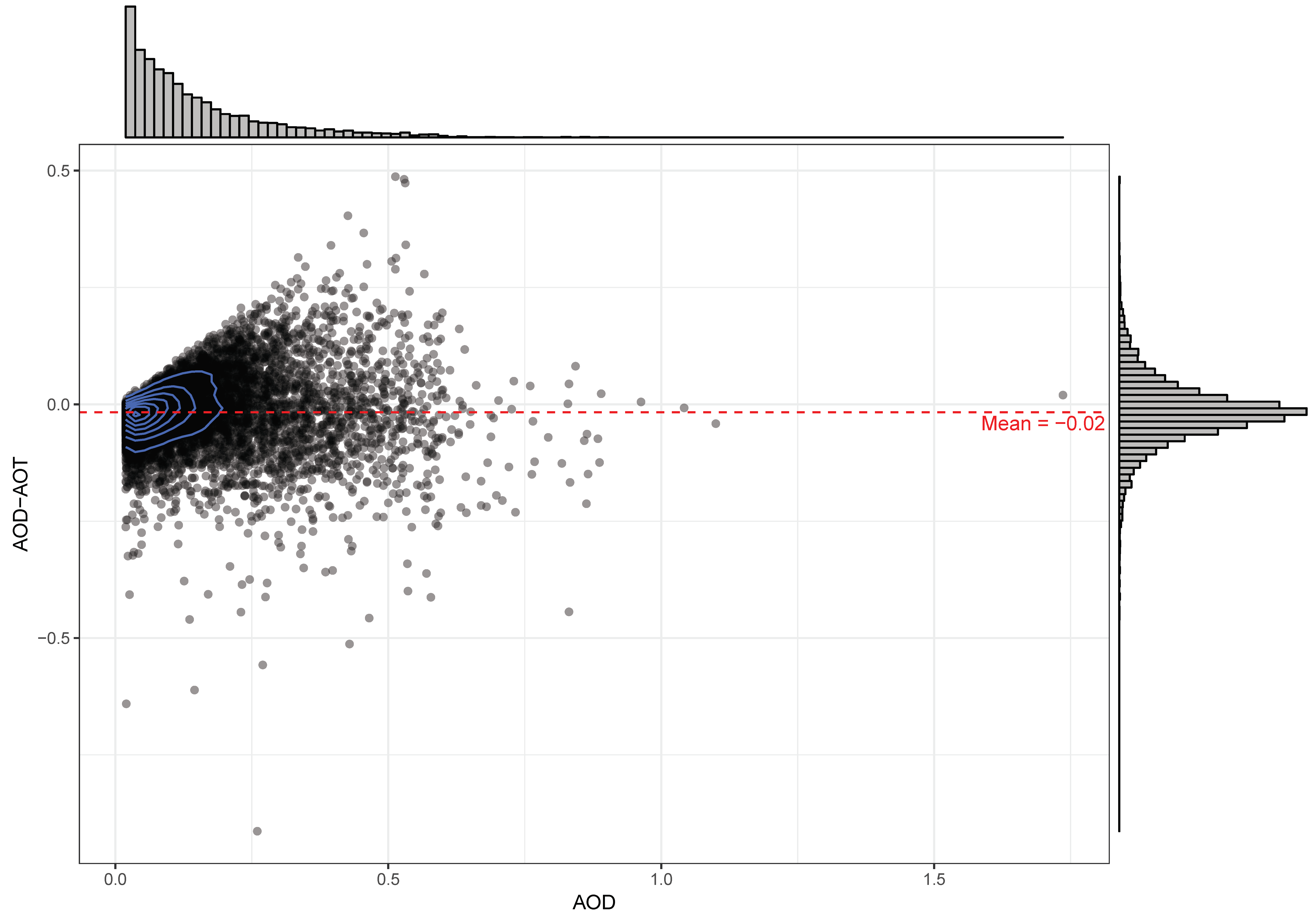
The Pearson correlation between AOD and AOT in the entire measurement error dataset was 0.86 and 0.89 for Aqua and Terra, respectively. The difference between AOD and AOT (AOD-AOT) had mean and range equal to −0.02 (−0.91, 0.49) and −0.01 (−0.61, 0.66) for Aqua and Terra, respectively (
Figure 2).
As described in Materials and Methods, we used three different ensemble learning methods to predict AOT starting from AOD. All models were trained on the training set and their performances were validated by computing the RMSPE on the testing set.
Table 2 shows the values of the RMSPE and R
2 for models predicting the parameter AOD-AOT in the testing sets for both Aqua and Terra, although the R
2 is not directly comparable between the Aqua and Terra datasets because they were built on different datasets and thus are not nested models. For all models, the value of the RMSPE was much lower (up to ~43%, with the best performance from XGBoost) than the root mean square difference between AOD and AOT (0.074 and 0.079 for Aqua and Terra, respectively).
Scatterplots showing the agreement of the XGBoost-corrected data versus the original MAIAC values on the testing set are shown in
Figure S1. There is still a strong agreement of the raw AOD and the corrected AOD after applying the measurement error prediction, suggesting that the changes are not drastic with the majority of predictions remaining very similar to their original AOD values. When the XGBoost predicted measurement error model was applied to correct all nearly 50 million non-missing AOD observations for 2008 on Aqua in the full study region, the median absolute difference between the original and corrected AOD was 0.038 and only two percent of observations had an absolute change greater than the interquartile range of the AOD dataset (0.146).
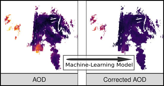
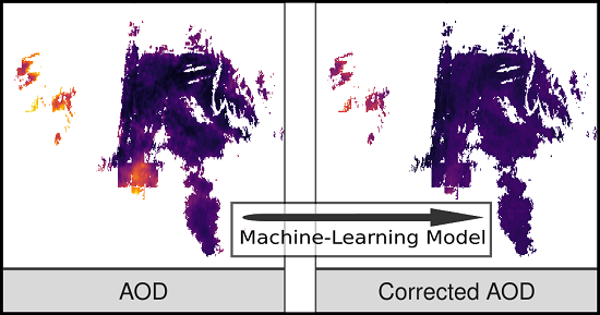
As a visual example of the impact of applying this approach to MAIAC AOD, we generated maps for 16 January 2008 (a testing set day not used in model training) showing the non-missing AOD from the southwestern portion of the region before and after applying the XGBoost model correction (
Figure 3). The correction pulls down the right tail of the AOD distribution leading to greater homogeneity in this scene and particularly attenuates some of the higher values seen in small clusters on the left or close to edges that are likely near clouds.
Although all three ensemble approaches use different measures of variable importance, there was generally high agreement in the rank of the variable importance (
Figure S2), with several features showing up among the most important in all three modeling approaches for both Aqua and Terra: relative azimuth, AOT uncertainty, long term time trend, windowed differences of AOD over smaller to intermediate scales of 30 km to 210 km, and column water vapor (
Figure 4). In general, there was good agreement in the rank of the most and least important variables including the lowest importance for MAIAC cloud mask, which arises infrequently in the data collocated with AERONET measures, and the MAIAC aerosol model flag for dust-affected values. Both of these two variables have little variation in the measurement error dataset over this particular study region. There was less consistency in variable importance rank between modeling approaches for the majority of variables assigned a more intermediate importance.
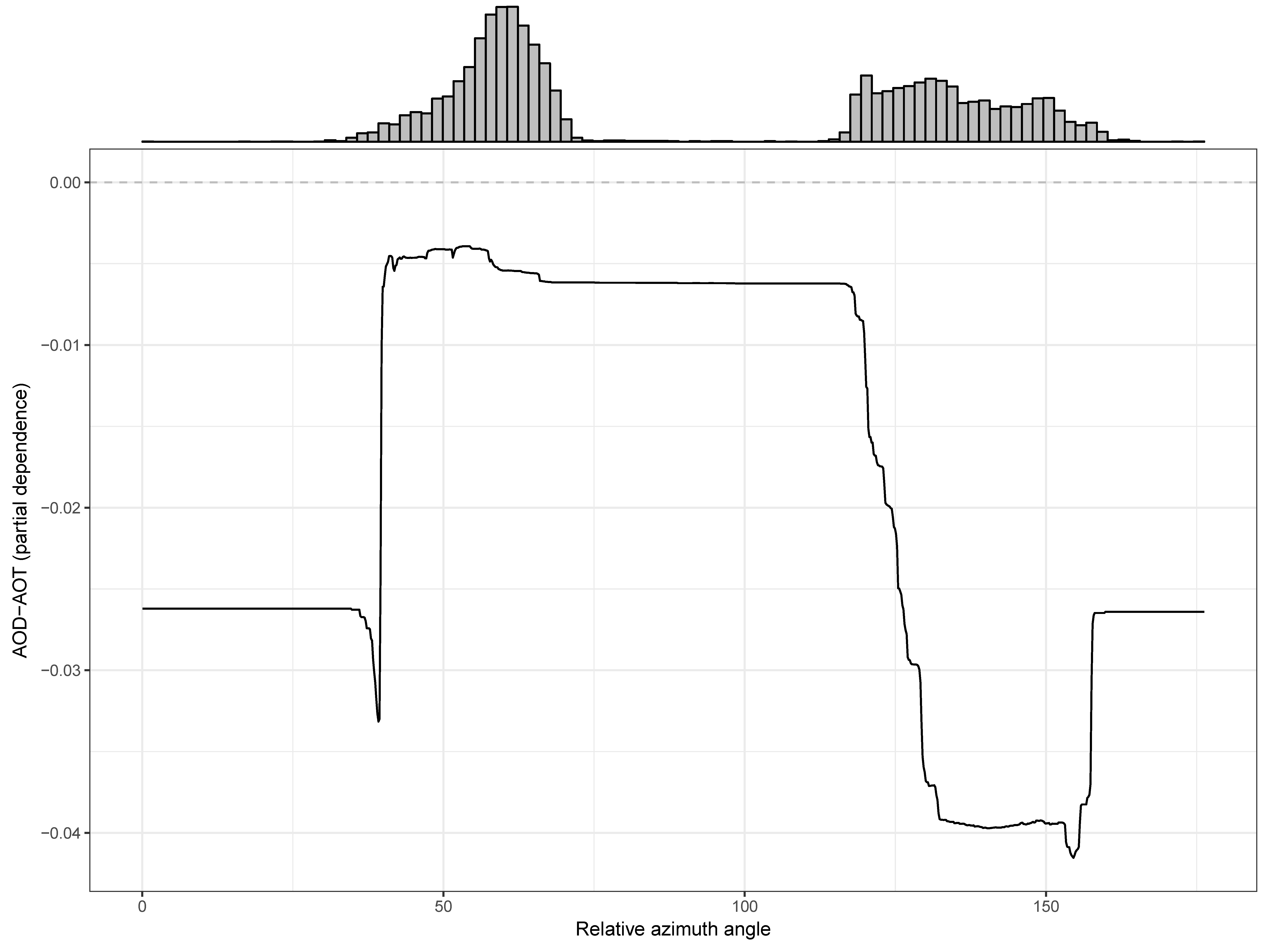
Partial dependence plots were used to visualize the relation of the most important features with the measurement error parameter (
Figure 5 and
Figure S3–S5).
To assess whether a simpler model (using fewer features) could achieve similar prediction performance, we also re-fit XGBoost on the Aqua dataset using just the top 10 or top 20 most important predictors from the full XGBoost model. The RMSPE of the testing set was equal to 0.050 (19% worse than the full model) and 0.047 (12% worse than the full model) for models fit with only the top 10 and 20 covariates, respectively.
To reflect predictive uncertainty in our machine-learning models, in addition to predicting corrected AOD, we generated multiple imputation datasets for corrected AOD. This was done both by bootstrapping the original training dataset (RF and XGBoost) or applying the infinitesimal jackknife (IJ) method to estimate variances for each prediction from the RF model only. In all three methods, the variance of the predictions was larger when the absolute difference between AOD and AOT was larger (data not shown).
Because AOD is used as an important predictor in pollution models that estimate ground-level PM
2.5, the raw and corrected AOD were correlated with PM
2.5 across a network of ground monitoring stations independent of the AERONET AOT. The Pearson correlation between PM
2.5 and raw MAIAC AOD was equal to 0.47 and 0.56 for Aqua and Terra, respectively. After correcting the MAIAC AOD using our XGBoost model, the correlations went up to 0.57 and 0.65 for Aqua and Terra, respectively (
Table 3). Using Rubin’s rule to combine multiple imputations after a z-transformation [
20], the resulting point estimates were the same, with the mean of the correlation between PM
2.5 and 5 imputed versions of the XGBoost predicted values of AOT equal to 0.57 (sd = 0.003) and 0.65 (sd = 0.002) for Aqua and Terra, respectively.
4. Discussion
There is a growing record of remote sensing products from an increasing number of sensors, including forthcoming high-resolution sub-hourly coverage from geostationary platforms such as Himawari 8 and GOES-16 [
21,
22]. The volume of such data makes it possible to construct complex exposure models covering large regions, but also makes the cleaning of these data a challenge with an overwhelming volume of data to visualize and an increasing number of quality metrics to integrate.
We present a machine-learning approach to address measurement error in MAIAC retrievals, a leading AOD product, that makes data cleaning scalable, even when addressing large regions and many years of data. An advantage of adding a measurement error model is that a corrected value can be output as a prediction without reducing the size of the dataset, as is often done when excluding data points with problematic quality control parameters. Thus, this approach can be applied in a two-stage modeling framework where the corrected AOD value is available for further applications such as air pollution modeling or emissions inventories. Using a measurement error framework to correct AOD in this way is novel and differs from previous applications in which machine-learning methods have used uncorrected AOD products as predictors in estimating ground-level air pollutants without first addressing measurement error in AOD [
23,
24].
When predictions of AOD-AOT are evaluated on a withheld testing set, all three ensemble learning approaches improve on the MAIAC AOD with lower RMSPE for both Aqua and Terra. In both datasets, as expected, the XGBoost model which includes important features of both the Random Forest (random feature subsampling) and the gradient boosting approach outperforms the GBM, which outperforms the RF, in terms of lower RMSPE and higher R2. The additional performance of the gradient boosting approaches GBM and XGBoost over the simpler RF approach requires additional model hyperparameters related to the learning rate and feature subsampling (XGBoost only), but our model tuning suggests that the improved performance of the XGBoost may be due to those additional model characteristics. Comparing raw AOD and predicted AOT with the observed AOT in the testing set, the mode of the AOT is slightly higher and the density is more peaked, although both datasets have a long right tail. The prediction model does not drastically shrink high values as we might have expected if they were due to large systematic errors, such as from cloud contamination as opposed to the long-range transport of smoke from biomass burning, although the training dataset included few truly high AOD values (>1).
While flexible ensemble learning methods are quite performant and lead to excellent predictive performance in data science challenges [
25,
26], they are sometimes criticized as being less interpretable than a more parsimonious or parametric approach. Variable importance metrics and partial dependence plots can summarize essential relationships and improve the understanding of complex predictive models. For example, the Relative Azimuth (RA) was shown in all three modeling strategies to be one of the most important predictor variables in the variable importance metrics and the partial dependence plot demonstrates that the larger contribution to measurement error occurs when the RA has an angle of >120° in backscattering conditions (which is almost half of the data). This data-driven result is consistent with our expectation of higher error in estimating aerosols in backscattering conditions (when the satellite is oriented between the sun and the earth’s surface) because of a lack of shadows and greater surface brightness that are challenging for aerosol retrieval algorithms [
3]. Thus these strategies help to understand how our empirical/statistical findings fit with the physical model underlying the MAIAC retrieval approach and may lead to future contributions in the MAIAC algorithm.
There are multiple methods to estimate variable importance in ensemble learning models. While there was great agreement in the most and least important variables across the three methods we employed, there was some heterogeneity in the rank of the importance of the intermediate variables across methods and with different variable importance metrics. For example, the permutation importance in the RF model, which is known to have difficulty with highly correlated predictors [
27], quantified the many different windowed variables (from a highly correlated set of predictors) as much less important than the RF variable importance based on minimal depth, which was in turn highly correlated with the rank importance of the XGBoost model variable importance from node purity (
Figure S2).
A major motivation in the feature engineering was to capture aspects of the data that might explain aberrant values seen when plotting individual satellite overpass scenes. For example, the variable “distance to edge”, which measures the distance of a non-missing pixel to the nearest missing pixel, was developed to capture edge effects that might be related to incomplete cloud masking. However, this feature was not as important as variables derived from the anomaly of AOD from moving windows as well as fixed geographic regions, taking advantage of the spatial autocorrelation and generally high homogeneity of AOD measures within a given scene in the Northeastern and Mid-Atlantic USA. Another counter-intuitive finding is that the partial dependence plot for the long-term time trend (operationalized as integer date) suggests that the measurement error in this dataset has been decreasing with time, even though the sensors in the MODIS platform have been aging with an expected decrease in accuracy since their deployment aboard the Aqua and Terra satellites. However, the time trend may be showing patterns in the residual after the removal of the calibration trend from the raw MODIS measurements prior to the application of the MAIAC retrieval algorithm [
28].
Given the large number of features considered in these measurement error models, it might be of interest to consider simplifying this approach in future applications by leaving out features that had a low variable importance and that required processing extra data sources. When we ran the XGBoost model with only the top 10 or 20 predictors, there was a moderate decrease in the improvement in measurement error achieved in the testing set. This tradeoff makes sense given that many of the included features had similar and intermediate variable importance measures.
As we propose using a statistical model to update AOD measures, it may be useful to estimate the uncertainty in these predictions as well. While the properties of the Infinitesimal Jackknife (IJ) for estimating predictive uncertainty of estimates from Random Forest models have been previously demonstrated [
15], more work is needed to approximate the posterior predictive distribution for other ensemble methods, such as XGBoost. When the same Random Forest model was used to compare the estimated variance of the predictions between bootstrapping and the Infinitesimal Jackknife, we found that the correlation was moderate for variance estimates after only 5 bootstrap resamplings (r = 0.78 excluding a single outlier) and went up further when the variance estimates were computed after resampling 50 times (r = 0.89 excluding a single outlier). A future direction of this work would be to use estimates of the predictive uncertainty in further analyses that employ the corrected AOD values as a predictor of ground-level PM
2.5, perhaps by adapting multiple-imputation approaches for measurement error correction [
19].
Although our approach to address measurement error in satellite AOD is novel and shows a substantial improvement in the resulting product, it has several limitations. The temporal and spatial coverage of the AERONET dataset used for validation is not representative of the entire space-time domain of interest (e.g., the majority of unique AERONET sites are in urban areas; particularly the DRAGON snapshot campaign in the DC area [
29]). Furthermore, because only cloud-screened and quality-assured AERONET station data are used as a reference value for AOD, the most problematic measurements (e.g., when there is a nearby cloud) for satellite-based AOD measures may be underrepresented in our validation dataset making it difficult to train the model to correct these largest outliers. For example, there are few data points in our validation dataset that have very high AOD (AERONET AOT >1.5 only once in Aqua and twice in Terra in our dataset) because true values this large occur only rarely in this region, even though it is not as uncommon in the MAIAC dataset. Given the differences in the overall MAIAC dataset and the subset we use for measurement error correction (collocated with AERONET), future models may be improved by implementing inverse probability weighting of the measurement error dataset back to the originating dataset. Finally, the AERONET measure represents a measurement of AOD at a single point, while the AOD from MAIAC is an estimate over a 1 km
2 region, and this can contribute to spatial/temporal misalignment that we have captured within our estimation of measurement error. While our application benefited from a reasonably large number of AERONET stations in the Northeastern USA, this approach has not yet been tested in regions which have few AERONET stations. A future direction for this work will be to examine the generalizability of this approach in other regions (leveraging the global coverage of MAIAC and the AERONET station network) and particularly examine performance where there are fewer unique AERONET stations and collocated observations.
Although extreme (high) values of AOD are relatively rare, these values merit extra attention as they may indicate unusual pollutant scenarios or highly influential outliers if not real. We discovered that for the Aqua satellite, the highest pair of AOD and AOT data points in our collocated measurement error dataset occurred on 10 June 2015 after long range drift of smoke from Canadian wildfires [
30]. However, the detection of emitted smoke that has undergone long-range transport is a challenge in the field and may be too infrequent in our measurement error dataset to make a meaningful contribution here.

 ,
, 


