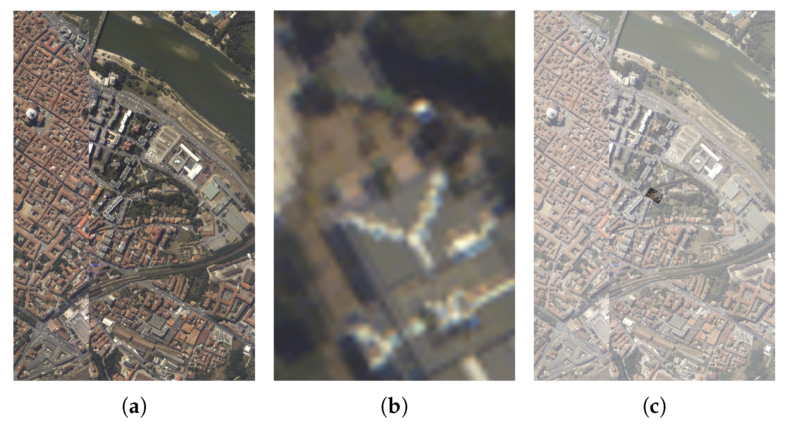
Figure 1.
Example of registration considered in this work: (a) Reference image (size , (b) Target image, and (c) Result of the registration process showing the correctly registered superposition of the reference and target registered image (scale and rotation angle 60).
Figure 1.
Example of registration considered in this work: (a) Reference image (size , (b) Target image, and (c) Result of the registration process showing the correctly registered superposition of the reference and target registered image (scale and rotation angle 60).
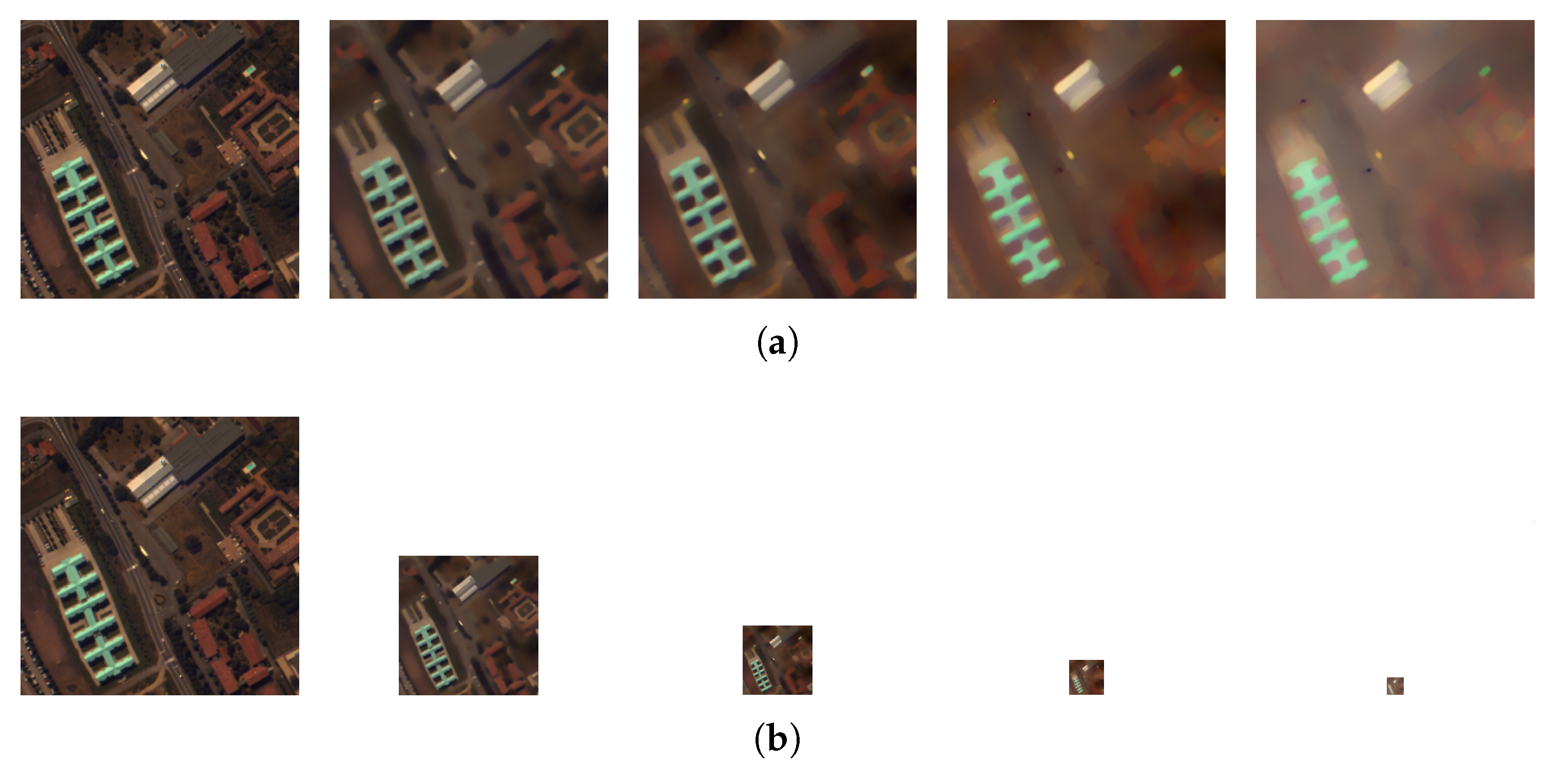
Figure 2.
(a) Scale space used by KAZE (b) Pyramidal scale space used by A–KAZE. Each image represents the first sublevel of the next octave.
Figure 2.
(a) Scale space used by KAZE (b) Pyramidal scale space used by A–KAZE. Each image represents the first sublevel of the next octave.
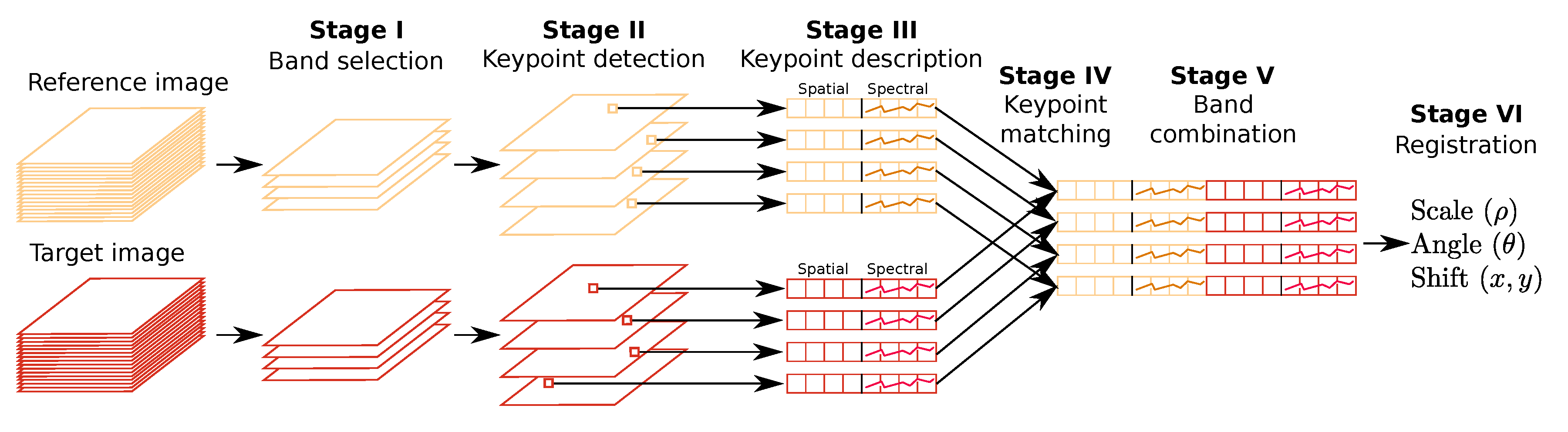
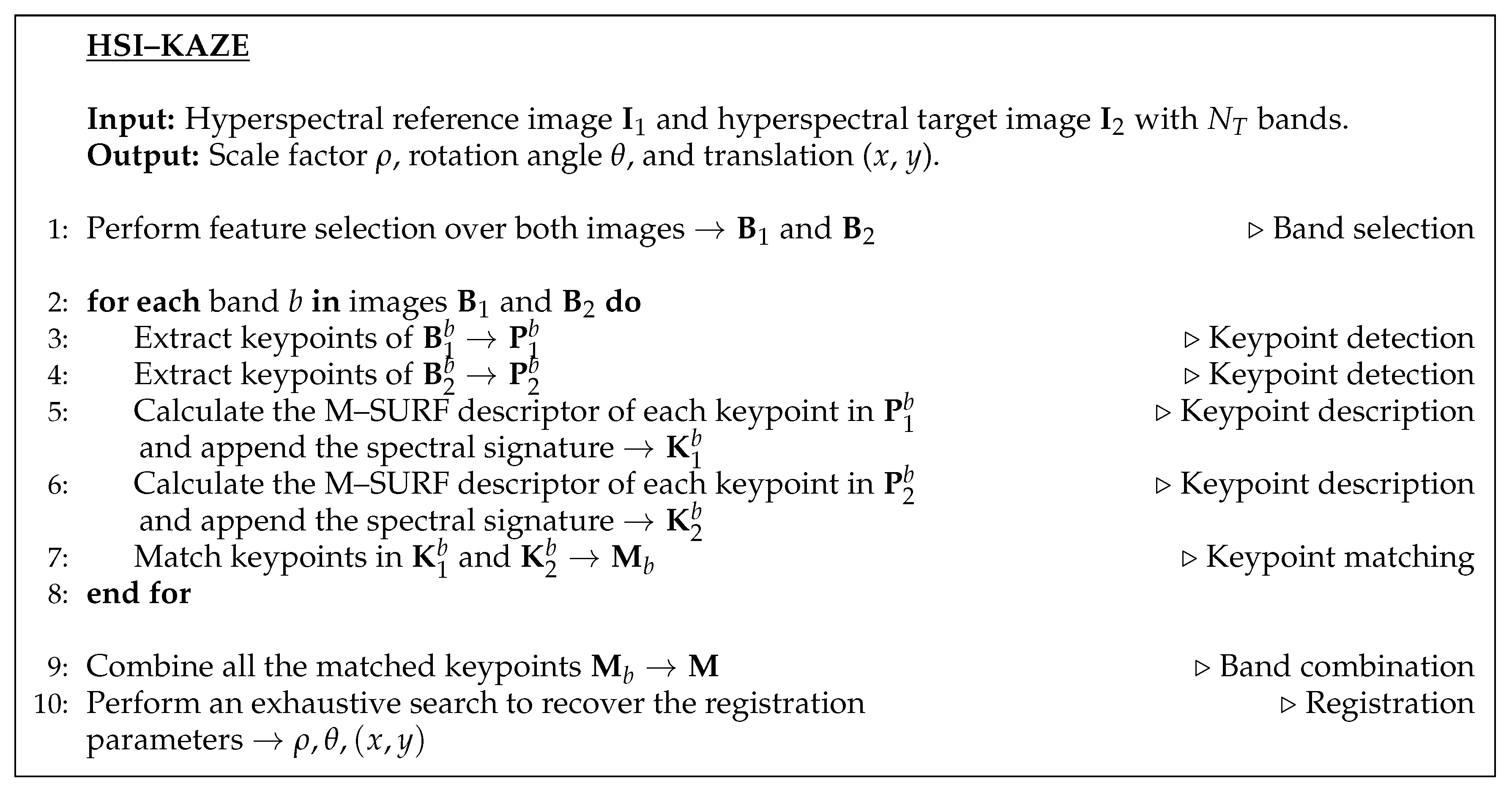
Figure 3.
HSI–KAZE algorithm to register two hyperspectral images.
Figure 3.
HSI–KAZE algorithm to register two hyperspectral images.
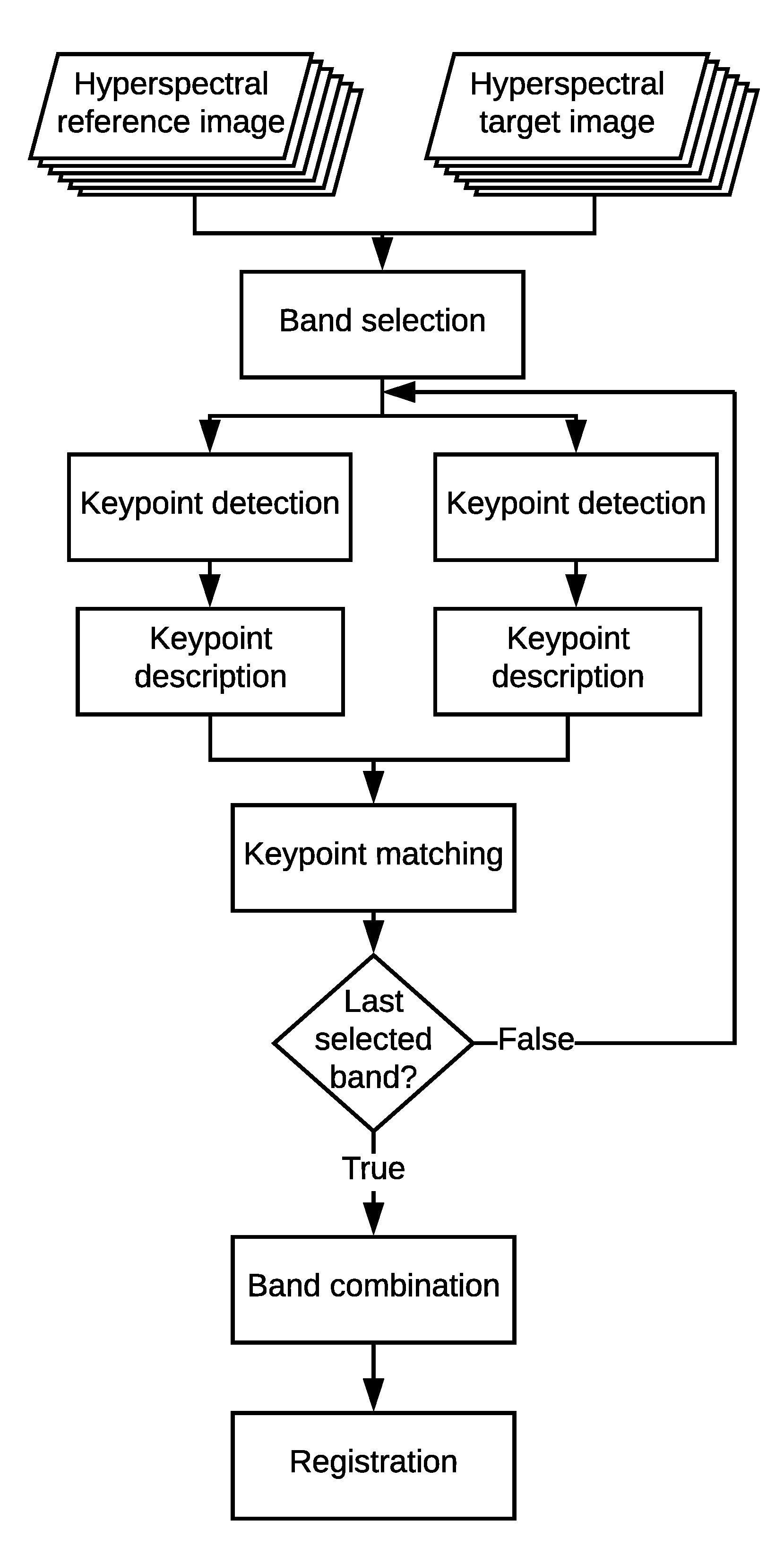
Figure 4.
Flow chart of the proposed HSI–KAZE algorithm to register two hyperspectral images.
Figure 4.
Flow chart of the proposed HSI–KAZE algorithm to register two hyperspectral images.
Figure 5.
HSI–KAZE pseudocode.
Figure 5.
HSI–KAZE pseudocode.
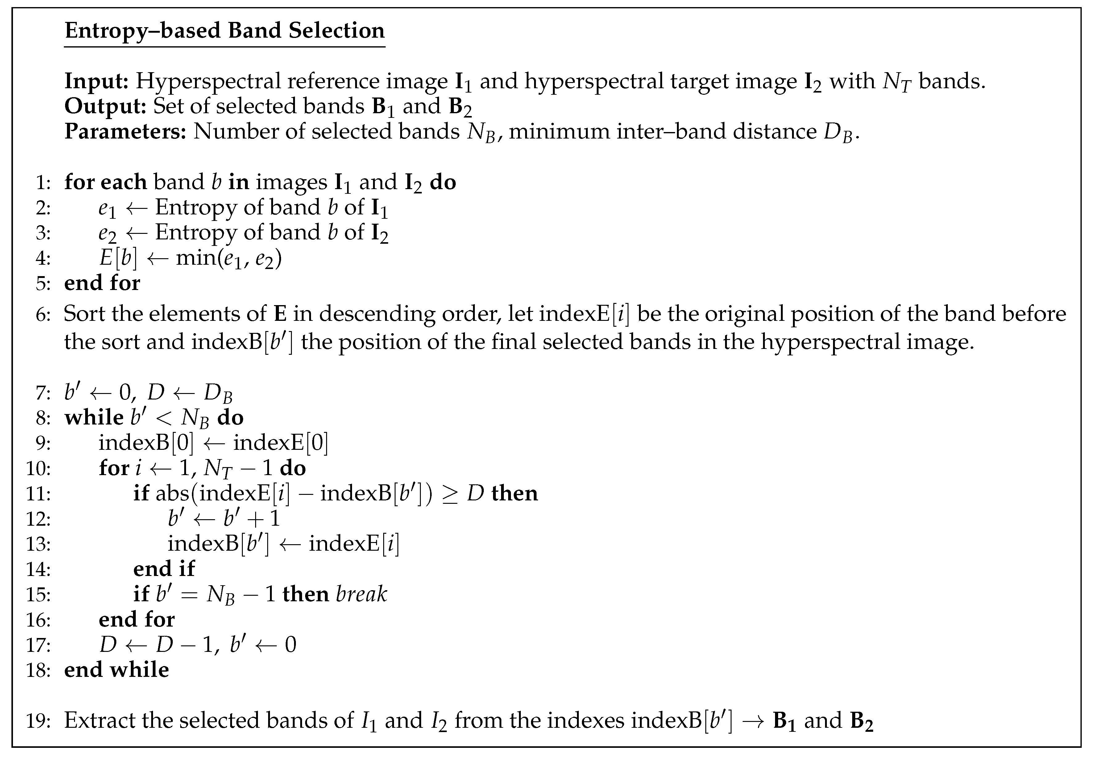
Figure 6.
Pseudocode for the band selection stage of the HSI–KAZE.
Figure 6.
Pseudocode for the band selection stage of the HSI–KAZE.
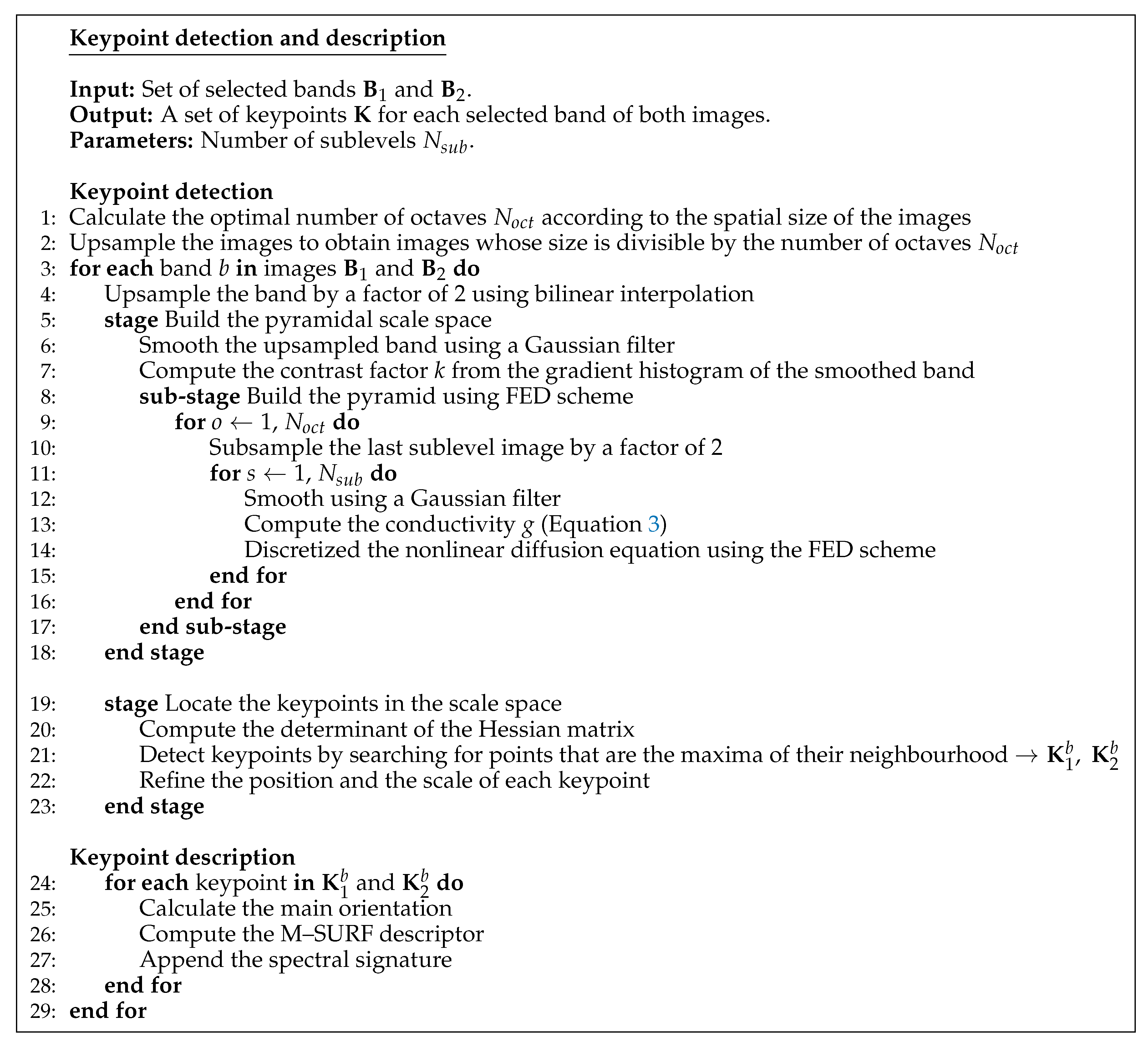
Figure 7.
Pseudocode for the keypoint detection and description stages of the HSI–KAZE.
Figure 7.
Pseudocode for the keypoint detection and description stages of the HSI–KAZE.
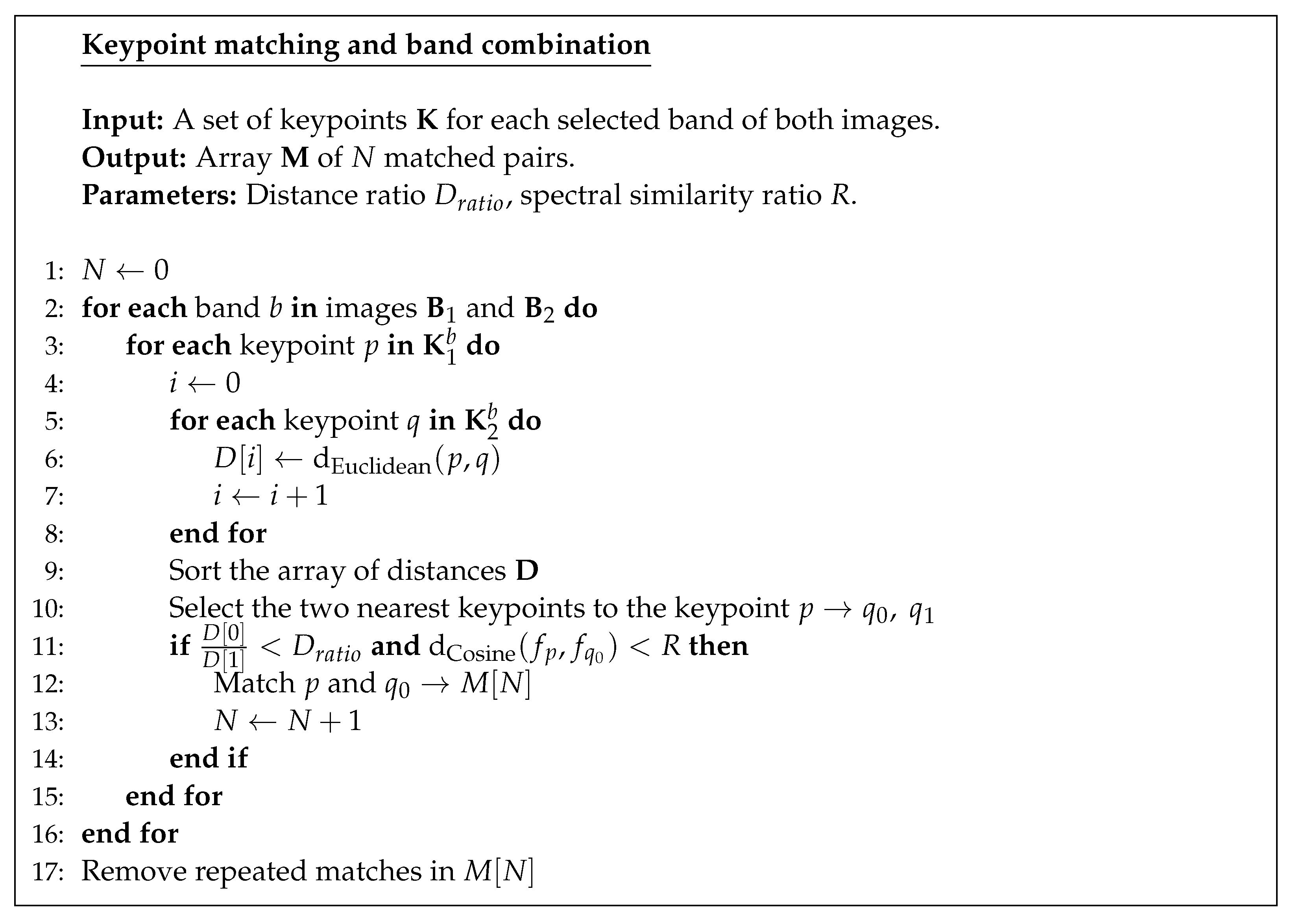
Figure 8.
Pseudocode for the keypoint matching and band combination.
Figure 8.
Pseudocode for the keypoint matching and band combination.
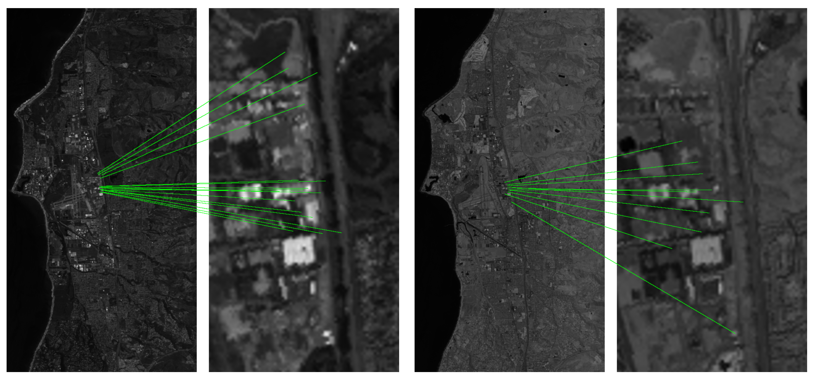
Figure 9.
Matched keypoints detected in two pairs of bands belonging to the Santa Barbara Front scene (bands 26 and 93 with scale ).
Figure 9.
Matched keypoints detected in two pairs of bands belonging to the Santa Barbara Front scene (bands 26 and 93 with scale ).
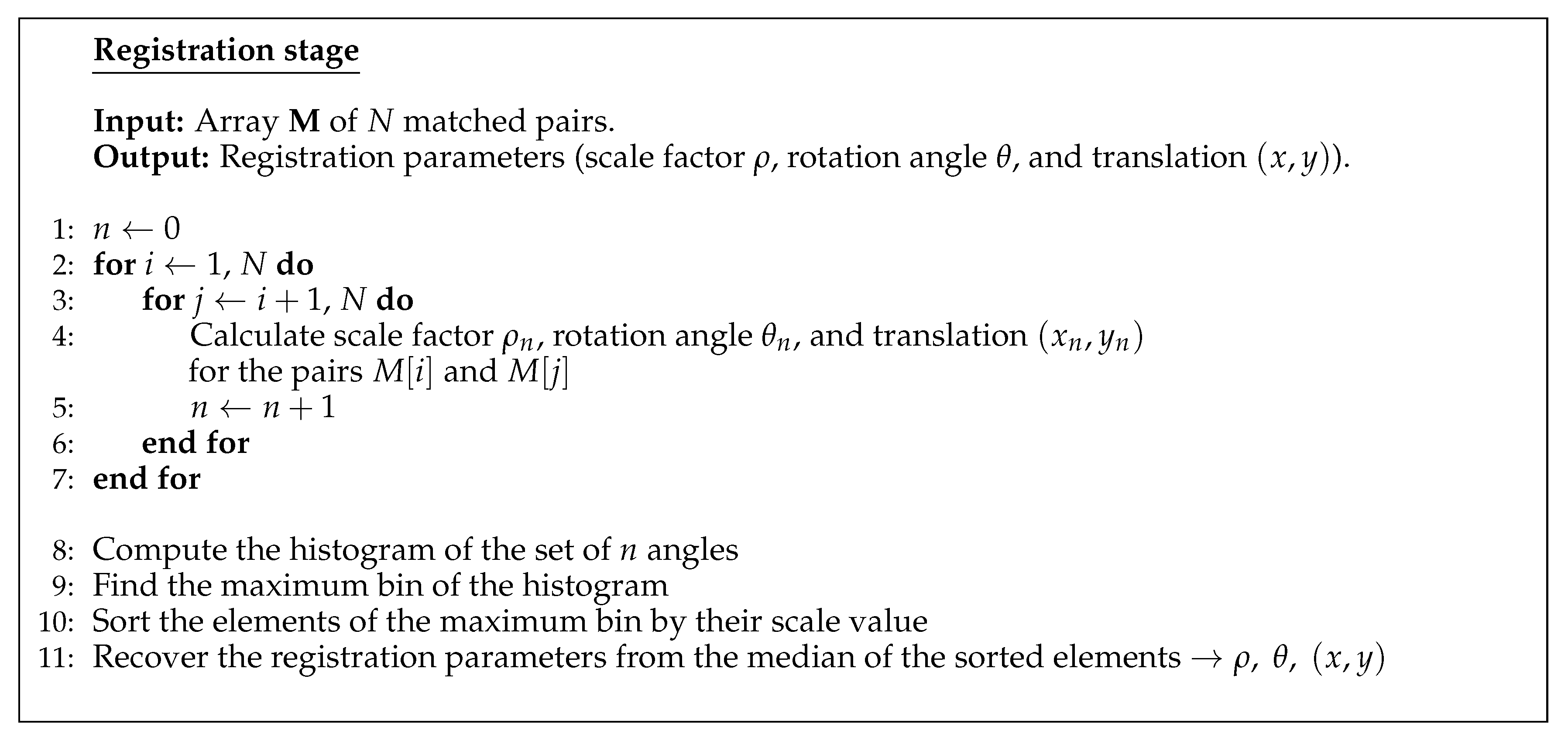
Figure 10.
Pseudocode for the registration stage of the HSI–KAZE.
Figure 10.
Pseudocode for the registration stage of the HSI–KAZE.
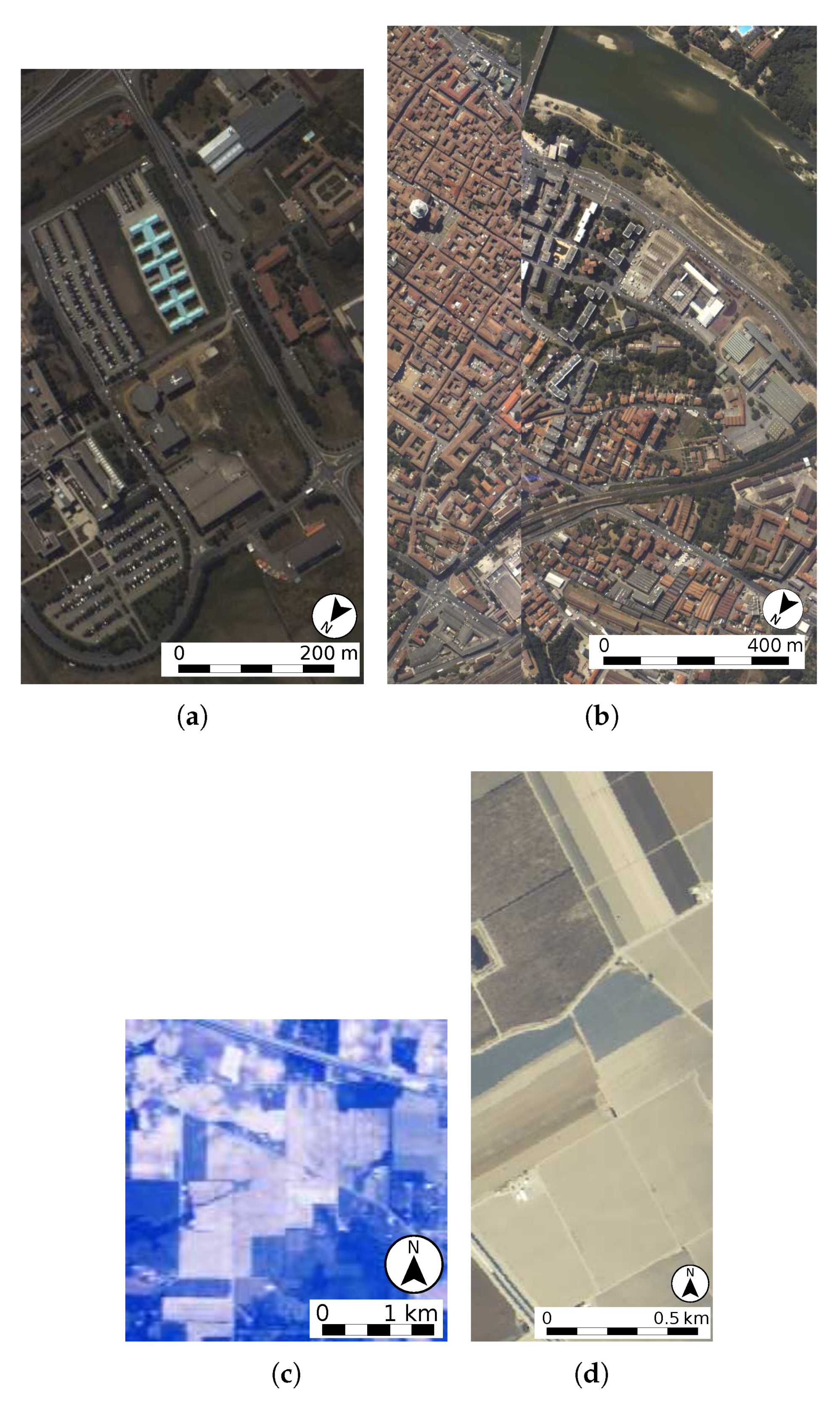
Figure 11.
Hyperspectral images commonly used for testing in remote sensing: (a) Pavia University, (b) Pavia Centre, (c) Indian Pines, and (d) Salinas.
Figure 11.
Hyperspectral images commonly used for testing in remote sensing: (a) Pavia University, (b) Pavia Centre, (c) Indian Pines, and (d) Salinas.
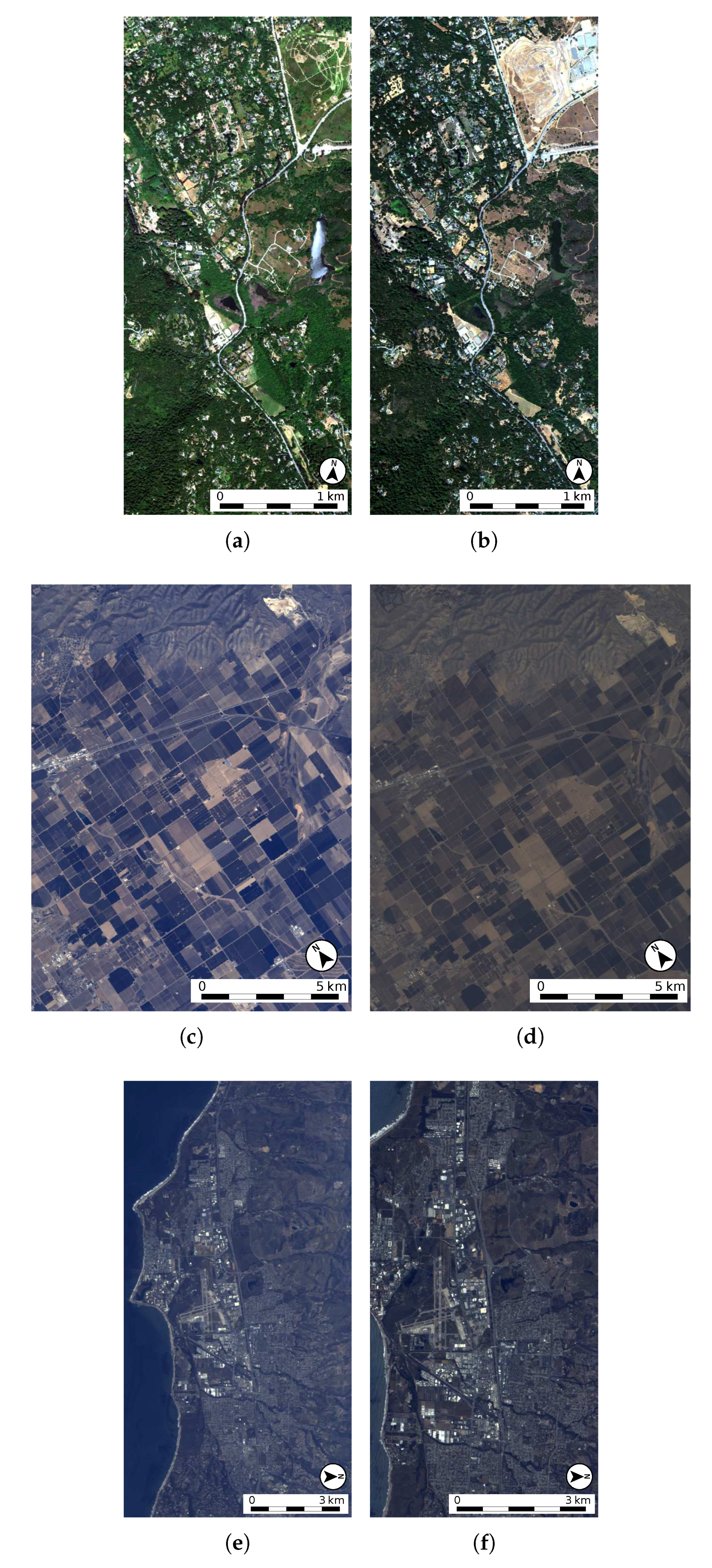
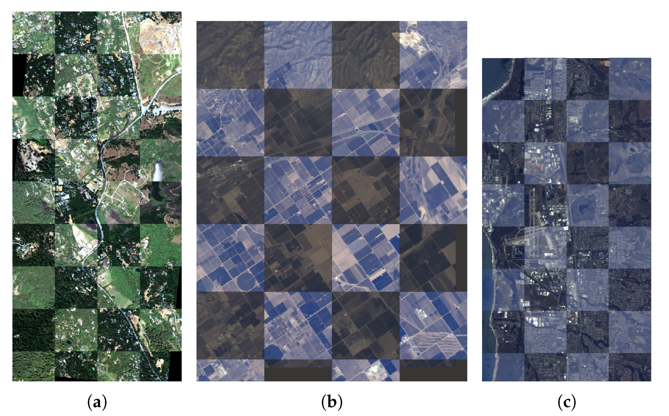
Figure 12.
Second group of the test hyperspectral images: (a) Reference Jasper Ridge image taken on 5 December 2006, (b) Target Jasper Ridge image taken on 13 August 2007, (c) Reference Santa Barbara Box image taken on 11 April 2013, (d) Target Santa Barbara Box image taken on 16 April 2014, (e) Reference Santa Barbara Front image taken on 30 March 2009, and (f) Target Santa Barbara Front image taken on 30 April 2010.
Figure 13.
Chequerboard registered images for the scenes taken by the AVIRIS sensor at different dates: (a) Jasper Ridge, (b) Santa Barbara Box, and (c) Santa Barbara Front.
Figure 13.
Chequerboard registered images for the scenes taken by the AVIRIS sensor at different dates: (a) Jasper Ridge, (b) Santa Barbara Box, and (c) Santa Barbara Front.
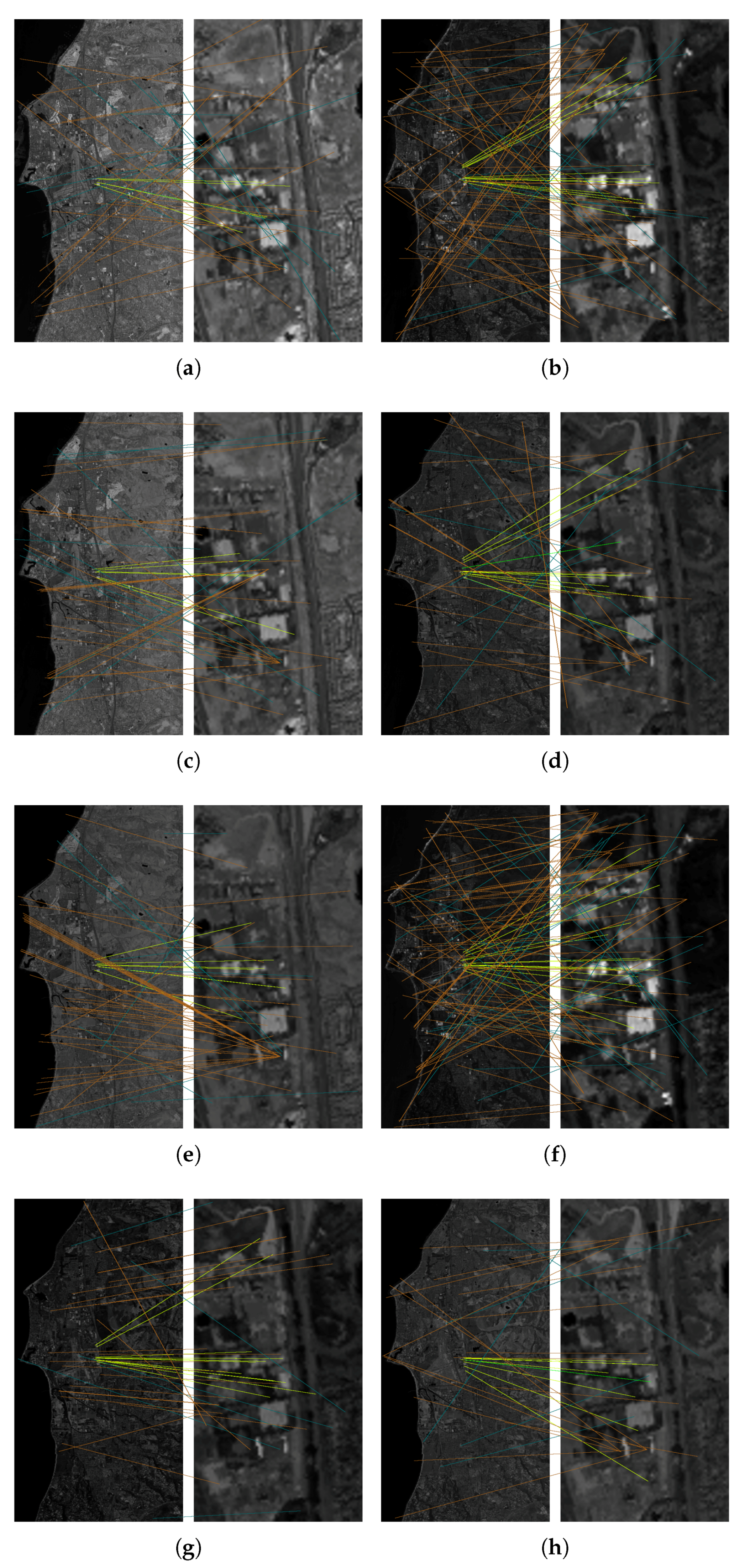
Figure 14.
Matched keypoints detected in the eight selected bands ordered by decreasing entropy from Santa Barbara Front scene with scale : (a) Band 46, (b) Band 26, (c) Band 71, (d) Band 126, (e) Band 93, (f) Band 6, (g) Band 185, and (h) Band 146. Matches discarded after considering spectral information (brown), incorrect matches (blue), correct matches (yellow), and correct matches used in registration (green).
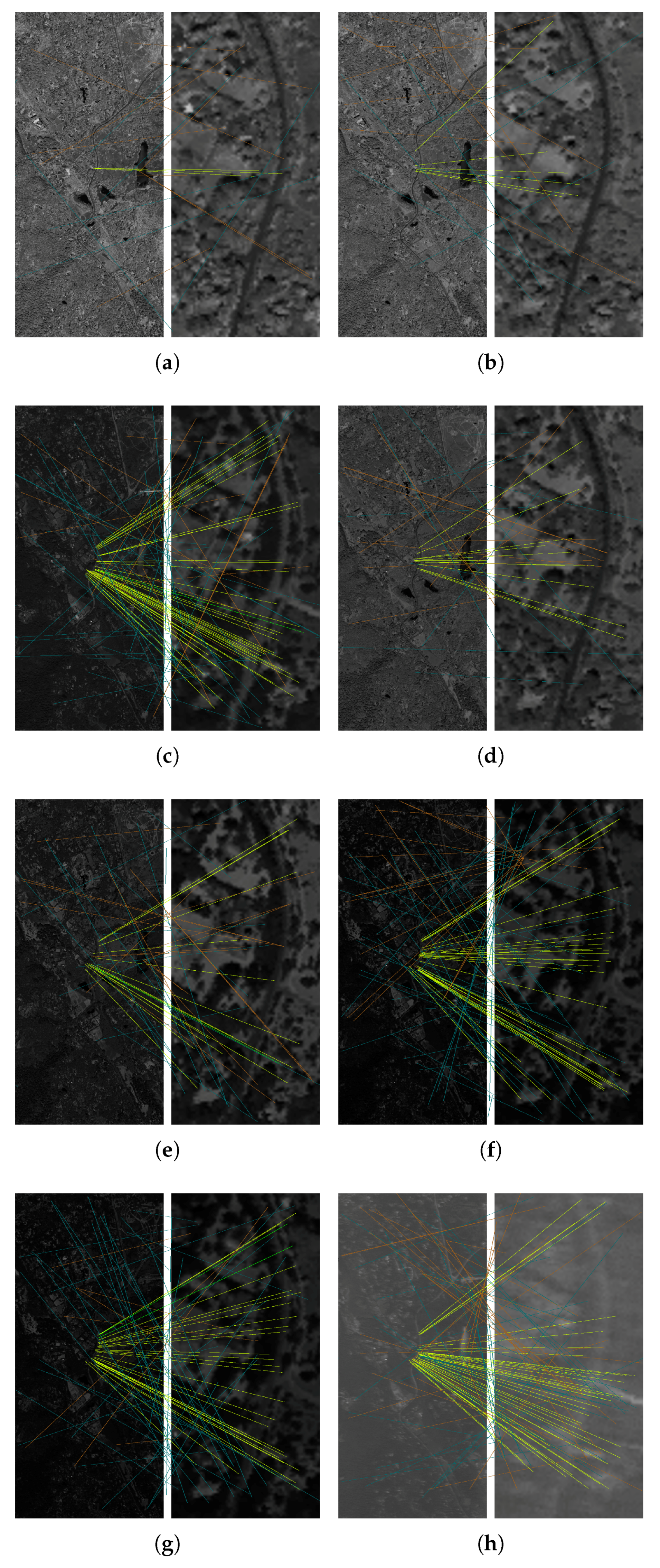
Figure 15.
Matched keypoints detected in the eight selected bands ordered by decreasing entropy from Jasper Ridge scene with scale : (a) Band 46, (b) Band 71, (c) Band 21, (d) Band 94, (e) Band 135, (f) Band 187, (g) Band 207, and (h) Band 1. Matches discarded after considering spectral information (brown), incorrect matches (blue), correct matches (yellow), and correct matches used in registration (green).
Table 1.
Sensor, size, number of spectral bands, resolution (m/pixel), and location of the test hyperspectral images.
Table 1.
Sensor, size, number of spectral bands, resolution (m/pixel), and location of the test hyperspectral images.
| Image | Sensor | Size | Bands | Spatial
Resolution | Location |
|---|
| Pavia University | ROSIS–03 | | 103 | | N 451213.176, E 9811.108 |
| Pavia Centre | ROSIS–03 | | 102 | | N 451107.4, E 9834.8 |
| Indian Pines | AVIRIS | | 220 | 20 | Refer to [36] |
| Salinas Valley | AVIRIS | | 204 | | Refer to [36] |
| Jasper Ridge 2006 | AVIRIS | | 224 | | N 37248.5, W 1221442.2 |
| Jasper Ridge 2007 | AVIRIS | | 224 | | N 37248.5, W 1221442.2 |
| Santa Barbara Box 2013 | AVIRIS | | 224 | | N 351814.3, W 1185022.6 |
| Santa Barbara Box 2014 | AVIRIS | | 224 | | N 351814.3, W 1185022.6 |
| Santa Barbara Front 2009 | AVIRIS | | 224 | | N 342624.3, W 1195040.0 |
| Santa Barbara Front 2010 | AVIRIS | | 224 | | N 342624.3, W 1195040.0 |
Table 2.
Band limits of each cluster produced by BandClust for all the scenes.
Table 2.
Band limits of each cluster produced by BandClust for all the scenes.
| Scene | Band Limits of Each Cluster |
|---|
| Pavia University | 1–64, 65–103 |
| Pavia Centre | 1–23, 24–60, 61–102 |
| Indian Pines | 1–38, 39–60, 61–65, 66–79, 80–102, 103–116, 117–149, 150–160, 161–220 |
| Salinas | 1–11, 12–23, 24–33, 34–44, 45–61, 62–68, 69–78, 79–83, 84–104, 105–109, 110–121, 122–150, 151–155, 156–204 |
| Jasper Ridge | 1–14, 15–37, 38–88, 89–107, 108–111, 112–146, 147–154, 155–162, 163–175, 176–204, 205–209, 210–214, 215–224 |
| Santa Barbara Front | 1–15, 16–35, 36–63, 64–87, 88–114, 115–120, 121–174, 175–224 |
| Santa Barbara Box | 1–6, 7–36, 37–44, 45–65, 66–71, 72–85, 86–99, 100–125, 126–134, 135–138, 139–152, 153–157, 158–160, 161–165, 166–224 |
Table 3.
Successfully registered cases for each scene using HSI–KAZE with different feature reduction methods. The number in parentheses summarizes the number of scales that were correctly registered for all angles. If an angle is incorrectly registered, the whole scale factor is considered incorrect, i.e., this case is not included in the table. The percentage values are calculated over 65, the number of scales considered.
| Scene | PCA | BandClust | WaLuMI | EBS |
|---|
| Pavia University | to | to | to | to |
| Pavia Centre | to | to | to | to |
| Indian Pines | to | to | to | to |
| Salinas | to | to | to | to |
| Jasper Ridge | to | to | to | to |
| Santa Barbara Front | to | to | to | to |
| Santa Barbara Box | to | to | to | to |
| Number of scalings (average) | () | () | () | () |
| Number of scalings (percentage) | | | | |
Table 4.
Successfully registered cases for each scene. The number in parentheses summarizes the number of scales that were correctly registered for all angles. If an angle is incorrectly registered, the whole scale factor is considered incorrect, i.e., this case is not included in the table. KAZE and A–KAZE are applied to the band with the highest entropy. KAZE and A–KAZE use RANSAC. The percentage values are calculated over 65, the number of scales considered.
| Scene | FMI–SPOMF | HYFM | KAZE (RANSAC) | A–KAZE (RANSAC) | HSI–KAZE |
|---|
| Pavia University | to | to | to | to | to |
| Pavia Centre | to | to | to | to | to |
| Indian Pines | to | to | to | | to |
| Salinas | to | to | to | to | to |
| Jasper Ridge | to | to | | | to |
| Santa Barbara Front | to | to | to | to | to |
| Santa Barbara Box | to | to | to | to | to |
| Number of scalings (average) | () | () | () | () | () |
| Number of scalings (percentage) | | | | | |
Table 5.
Successfully registered cases for each scene. The number in parentheses summarizes the number of scales that were correctly registered for all angles. If an angle is incorrectly registered, the whole scale factor is considered incorrect, i.e., this case is not included in the table. KAZE and A–KAZE are applied to the band with the highest entropy. In this case, KAZE and A–KAZE use the registration method proposed in HSI–KAZE. The percentage values are calculated over 65, the number of scales considered.
| Scene | FMI–SPOMF | HYFM | KAZE | A–KAZE | HSI–KAZE |
|---|
| Pavia University | to | to | to | to | to |
| Pavia Centre | to | to | to | to | to |
| Indian Pines | to | to | to | to | to |
| Salinas | to | to | to | to | to |
| Jasper Ridge | to | to | | to | to |
| Santa Barbara Front | to | to | to | to | to |
| Santa Barbara Box | to | to | to | to | to |
| Number of scalings (average) | () | () | () | () | () |
| Number of scalings (percentage) | | | | | |
Table 6.
Number and percentage of successfully registered cases for each scene and method for the entire test range (from to , 65 scale factors and 72 angles per scale).
Table 6.
Number and percentage of successfully registered cases for each scene and method for the entire test range (from to , 65 scale factors and 72 angles per scale).
| Scene | FMI–SPOMF | HYFM | KAZE | A–KAZE | HSI–KAZE |
|---|
| Pavia University | 999 (21.35%) | 1139 (24.34%) | 1446 (30.90%) | 856 (18.29%) | 2781 (59.42%) |
| Pavia Centre | 1268 (27.12%) | 1472 (31.45%) | 1859 (39.72%) | 1829 (39.08%) | 4647 (99.29%) |
| Indian Pines | 586 (12.52%) | 739 (15.79%) | 393 (08.40%) | 152 (03.25%) | 954 (20.38%) |
| Salinas | 876 (18.72%) | 856 (18.29%) | 907 (19.38%) | 625 (13.35%) | 1312 (28.03%) |
| Jasper Ridge | 663 (14.17%) | 697 (14.89%) | 148 (03.16%) | 352 (07.52%) | 2920 (62.39%) |
| Santa Barbara Front | 733 (15.66%) | 859 (18.35%) | 873 (18.65%) | 799 (17.07%) | 2404 (51.37%) |
| Santa Barbara Box | 508 (10.58%) | 948 (20.26%) | 715 (15.28%) | 720 (15.38%) | 2135 (45.62%) |
| Total successful cases | 5634 (17.20%) | 6710 (20.48%) | 6341 (19.36%) | 5333 (16.28%) | 17,153 (52.36%) |
Table 7.
The most common measures used to evaluate the effectiveness, accuracy and robustness of registration methods in the literature as well as the image type and the scale factor range considered.
Table 7.
The most common measures used to evaluate the effectiveness, accuracy and robustness of registration methods in the literature as well as the image type and the scale factor range considered.
| Ref. | Image Type | Scale Factor Range | Measures |
|---|
| [18] | Multispectral | to | Chequerboard, correct match rate, registration error |
| [19] | Multispectral | to | Chequerboard, correct match rate, RMSE |
| [20] | Multispectral | to | Correct match rate, number of matches |
| [21] | Multispectral | to | Correct match rate, number of correct matches, number of matches |
| [22] | Multispectral | | Number of correct matches |
| [40] | Multispectral and hyperspectral | | RMSE |
| [41] | Hyperspectral | | Registration error |
| [42] | Multispectral and hyperspectral | to | Chequerboard, number of correct matches, RMSE |
| [24] | Hyperspectral | | Number of keypoints, correct match rate |
| [43] | Multispectral | | Chequerboard, correct match rate, number of correct matches, RMSE |
| [44] | Multispectral and hyperspectral | | Correct match rate, number of correct matches, RMSE |
| [45] | Multispectral and panchromatic | to | RMSE |
| [46] | Multispectral | | Number of matches, RMSE |
| [47] | Multispectral | | Chequerboard, number of correct matches, RMSE |
| [48] | Multispectral | to | Registration error, chequerboard |
Table 8.
Reference registration parameters for the second group of the test hyperspectral images.
Table 8.
Reference registration parameters for the second group of the test hyperspectral images.
| Scene | Scale Factor | Rotation Angle (Degrees) | Translation (x,y) (Pixels) |
|---|
| Jasper | | | |
| Santa Barbara Front | | | |
| Santa Barbara Box | | | |
Table 9.
Comparisons of KAZE, A–KAZE and the proposed method HSI–KAZE regarding the original number of matches obtained for each scene.
Table 9.
Comparisons of KAZE, A–KAZE and the proposed method HSI–KAZE regarding the original number of matches obtained for each scene.
| | | KAZE | A–KAZE | HSI–KAZE |
|---|
| Jasper | Number of matches | 17 | 23 | 21,437 |
| Number of matches after spectral discarding | - | - | 21,105 |
| Number of matches after removing repeated matches | - | - | 20,860 |
| Number of correct matches | 13 | 18 | 20,535 |
| Santa Barbara Front | Number of matches | 207 | 328 | 44,550 |
| Number of matches after spectral discarding | - | - | 44,490 |
| Number of matches after removing repeated matches | - | - | 43,537 |
| Number of correct matches | 176 | 282 | 20,741 |
| Santa Barbara Box | Number of matches | 307 | 230 | 37,185 |
| Number of matches after spectral discarding | - | - | 37,001 |
| Number of matches after removing repeated matches | - | - | 36,314 |
| Number of correct matches | 234 | 171 | 18,502 |
Table 10.
Comparisons of KAZE, A–KAZE and the proposed method HSI–KAZE regarding the matches used to register the images.
Table 10.
Comparisons of KAZE, A–KAZE and the proposed method HSI–KAZE regarding the matches used to register the images.
| | | KAZE | A–KAZE | HSI–KAZE |
|---|
| Jasper | Number of matches used in registration | 17 | 22 | 4 |
| Number of correct matches used in registration | 13 | 18 | 4 |
| Correct match ratio | 0.76 | 0.82 | 1.00 |
| Santa Barbara Front | Number of matches used in registration | 185 | 262 | 4 |
| Number of correct matches used in registration | 165 | 234 | 4 |
| Correct match ratio | 0.89 | 0.89 | 1.00 |
| Santa Barbara Box | Number of matches used in registration | 241 | 221 | 4 |
| Number of correct matches used in registration | 204 | 170 | 4 |
| Correct match ratio | 0.85 | 0.77 | 1.00 |
Table 11.
Results in terms of RMSE and registration error for KAZE, A–KAZE and HSI–KAZE.
Table 11.
Results in terms of RMSE and registration error for KAZE, A–KAZE and HSI–KAZE.
| | | KAZE | A–KAZE | HSI–KAZE |
|---|
| Jasper | RMSE | 0.98 | 1.54 | 1.35 |
| Registration error (pixels) | 0.92 | 1.38 | 1.23 |
| Santa Barbara Front | RMSE | 1.33 | 1.37 | 1.44 |
| Registration error (pixels) | 1.16 | 1.18 | 1.42 |
| Santa Barbara Box | RMSE | 1.48 | 1.68 | 0.72 |
| Registration error (pixels) | 1.28 | 1.44 | 0.70 |
Table 12.
Execution times (in seconds) and memory requirements (in MiB) considering the last scale successfully registered in
Table 5 for each scene and method in CPU.
Table 12.
Execution times (in seconds) and memory requirements (in MiB) considering the last scale successfully registered in
Table 5 for each scene and method in CPU.
| Scene | FMI–SPOMF | HYFM | KAZE | A–KAZE | HSI–KAZE | Average |
|---|
| Pavia University | 30.64 s | 123.27 s | 1.53 s | 1.11 s | 67.38 s | 44.79 s |
| 30.70 MiB | 37.95 MiB | 238.26 MiB | 169.49 MiB | 121.40 MiB | 119.56 MiB |
| Pavia Centre | 136.99 s | 507.59 s | 6.56 s | 6.72 s | 454.98 s | 222.57 s |
| 114.83 MiB | 151.78 MiB | 547.93 MiB | 276.16 MiB | 482.22 MiB | 314.58 MiB |
| Indian Pines | 1.65 s | 6.59 s | 0.19 s | 0.10 s | 4.72 s | 2.65 s |
| 6.83 MiB | 6.83 MiB | 140.78 MiB | 130.05 MiB | 19.93 MiB | 60.88 MiB |
| Salinas | 6.89 s | 28.79 s | 0.94 s | 0.57 s | 22.71 s | 11.98 s |
| 32.62 MiB | 32.62 MiB | 188.17 MiB | 149.40 MiB | 40.57 MiB | 88.67 MiB |
| Jasper Ridge | 140.17 s | 508.71 s | 11.04 s | 12.80 s | 628.25 s | 260.19 s |
| 242.83 MiB | 242.83 MiB | 541.02 MiB | 272.57 MiB | 482.24 MiB | 356.30 MiB |
| Santa Barbara Front | 33.66 s | 120.87 s | 4.61 s | 4.50 s | 226.62 s | 78.05 s |
| 170.50 MiB | 184.50 MiB | 147.02 MiB | 209.09 MiB | 163.27 MiB | 174.88 MiB |
| Santa Barbara Box | 32.47 s | 121.93 s | 10.29 s | 11.00 s | 616.88 s | 158.51 s |
| 252.87 MiB | 252.87 MiB | 556.77 MiB | 278.06 MiB | 324.79 MiB | 333.07 MiB |
| Average | 54.64 s | 202.54 s | 5.02 s | 5.26 s | 288.79 s | 111.25 s |
| 121.60 MiB | 129.91 MiB | 337.14 MiB | 212.12 MiB | 233.49 MiB | 206.85 MiB |


