Modeling Gross Primary Production of a Typical Coastal Wetland in China Using MODIS Time Series and CO₂ Eddy Flux Tower Data

Abstract

How to effectively combine remote sensing data with the eddy covariance (EC) technique to accurately quantify gross primary production (GPP) in coastal wetlands has been a challenge and is also important and necessary for carbon (C) budgets assessment and climate change studies at larger scales. In this study, a satellite-based Vegetation Photosynthesis Model (VPM) combined with EC measurement and Moderate Resolution Imaging Spectroradiometer (MODIS) data was used to evaluate the phenological characteristics and the biophysical performance of MODIS-based vegetation indices (VIs) and the feasibility of the model for simulating GPP of coastal wetland ecosystems. The results showed that greenness-related and water-related VIs can better identify the green-up and the senescence phases of coastal wetland vegetation, corresponds well with the C uptake period and the phenological patterns that were delineated by GPP from EC tower (GPP_EC). Temperature can explain most of the seasonal variation in VIs and GPP_EC fluxes. Both enhanced vegetation index (EVI) and water-sensitive land surface water index (LSWI) have a higher predictive power for simulating GPP in this coastal wetland. The comparisons between modeled GPP (GPP_VPM) and GPP_EC indicated that VPM model can commendably simulate the trajectories of the seasonal dynamics of GPP_EC fluxes in terms of patterns and magnitudes, explaining about 85% of GPP_EC changes over the study years (p < 0.0001). The results also demonstrate the potential of satellite-driven VPM model for modeling C uptake at large spatial and temporal scales in coastal wetlands, which can provide valuable production data for the assessment of global wetland C sink/source.

1. Introduction

As a staggered transition zone of terrestrial ecosystem and marine ecosystem, coastal wetland constitutes chains of marshes and swamps, and provides valuable ecosystem services and benefits to human [1,2,3,4]. It plays an important role in the principal interchanges of material and energy and the global sequestration of carbon (C) [1,5,6]. As the key component of the C cycle, gross primary production (GPP) represents the capacity of vegetation to uptake C from the atmosphere [7,8,9,10]. However, global-scale and measurement-based estimation of the historical growth in GPP is still lacking. The dynamics of GPP in coastal wetlands and its response to global climate change is poorly quantified and understood [5,11,12]. Therefore, accurate quantification of GPP for coastal wetlands at various spatial and temporal scales is crucial and necessary for global C budgets assessment and climate change studies [13].

The eddy covariance (EC) method and remote sensing (RS) technology have greatly increased the opportunities for the quantification of GPP at regional or global scales. The EC method can continuously and reliably measure net exchanges of C, water and energy between atmosphere, and terrestrial ecosystems at the diurnal, seasonal, and annual scales [14,15,16,17]. It can be used for calibrating and validating ecological models by providing important information that is associated with photosynthetic period and GPP at the ecosystem scale [18,19,20]. However, C flux data provided by the EC method is limited by footprints (typically ranging from hundreds of meters to 1 km) and short time periods [21,22,23,24]. Satellite RS technology can alternatively provide rapid, continuous, systematic, and repetitive measurement of vegetation structure and function characterization over large areas [23,25]. It is an effective and powerful tool for monitoring properties of land surface and obtaining spatiotemporal information, and then estimating regional GPP and net primary production (NPP), which can be consistent with the EC tower footprint [26,27]. However, there is still lacking interrelated links and bridges between EC and RS.

The satellite-based model is the interrelated links and bridges between EC measurement and RS data at regional scale. Among many RS models, the production efficiency models (PEM) are widely used in the GPP estimation study because of its lesser number of driving parameters, accurate estimation, and the easier coupling of EC and RS [23,28,29,30,31]. These models generally predict GPP by light use efficiency (ε_g), photosynthetically active radiation (PAR), the fraction of the absorbed PAR by the vegetation canopy (FAPAR), and a greenness-related Normalized Difference Vegetation Index (NDVI) [32]. Recently, Xiao et al., has developed a RS-based vegetation photosynthesis model (VPM) to simulate GPP [33,34,35]. VPM is a well-established GPP model by the conceptual partitioning of chlorophyll and non-photosynthetically active vegetation within the canopy to simulate GPP [36]. The model used additional spectral bands, such as blue and shortwave infrared bands to calculate the Enhanced Vegetation Index (EVI) [37] and Land Surface Water Index (LSWI) [33,36,38]. For example, Li et al., used the improved EVI and LSWI as input data for the VPM model to better characterize the dynamics of vegetation. They also simulated GPP more accurately than other PEM models, which only used NDVI in Qinghai–Tibetan Plateau, China [23]. Recently, this model has been further developed and applied to several ecosystems, including forest, grassland, agriculture, and alpine wetland ecosystems [10,13,15,23,33,36,39,40], which demonstrated the potential to scale up in situ observations of GPP from the CO₂ flux tower sites.

As the largest wetland ecosystem in the warm temperate zone of China, the Yellow River Delta Wetland is the most active area of atmosphere-land-ocean interaction in the world [41,42,43,44]. Therefore, the accurate estimation of the C source/sink function and its influence mechanism for the targeted coastal wetland will help to quantify the interactions and feedbacks between global climate change and coastal wetland ecosystems. In this study, we have combined the analysis of EC flux data with remote sensing images in the Yellow River Delta during 2009–2010. We aim to: (i) characterize seasonal dynamics of reed by analyzing the Moderate Resolution Imaging Spectroradiometer (MODIS) vegetation indices (VIs) and CO₂ fluxes data; (ii) examine the biophysical expression of VIs related to seasonal dynamics of observed GPP data; and, (iii) evaluate the dependability and the applicability of the VPM model for simulating GPP of coastal wetland ecosystems. We also conducted a variety of uncertainty analysis for the model simulations. This study could help to deepen our understanding of C budgets of coastal wetland and further improve the potential of RS technology for monitoring and simulating the dynamics of regional vegetation and C fluxes.

2. Materials and Methods

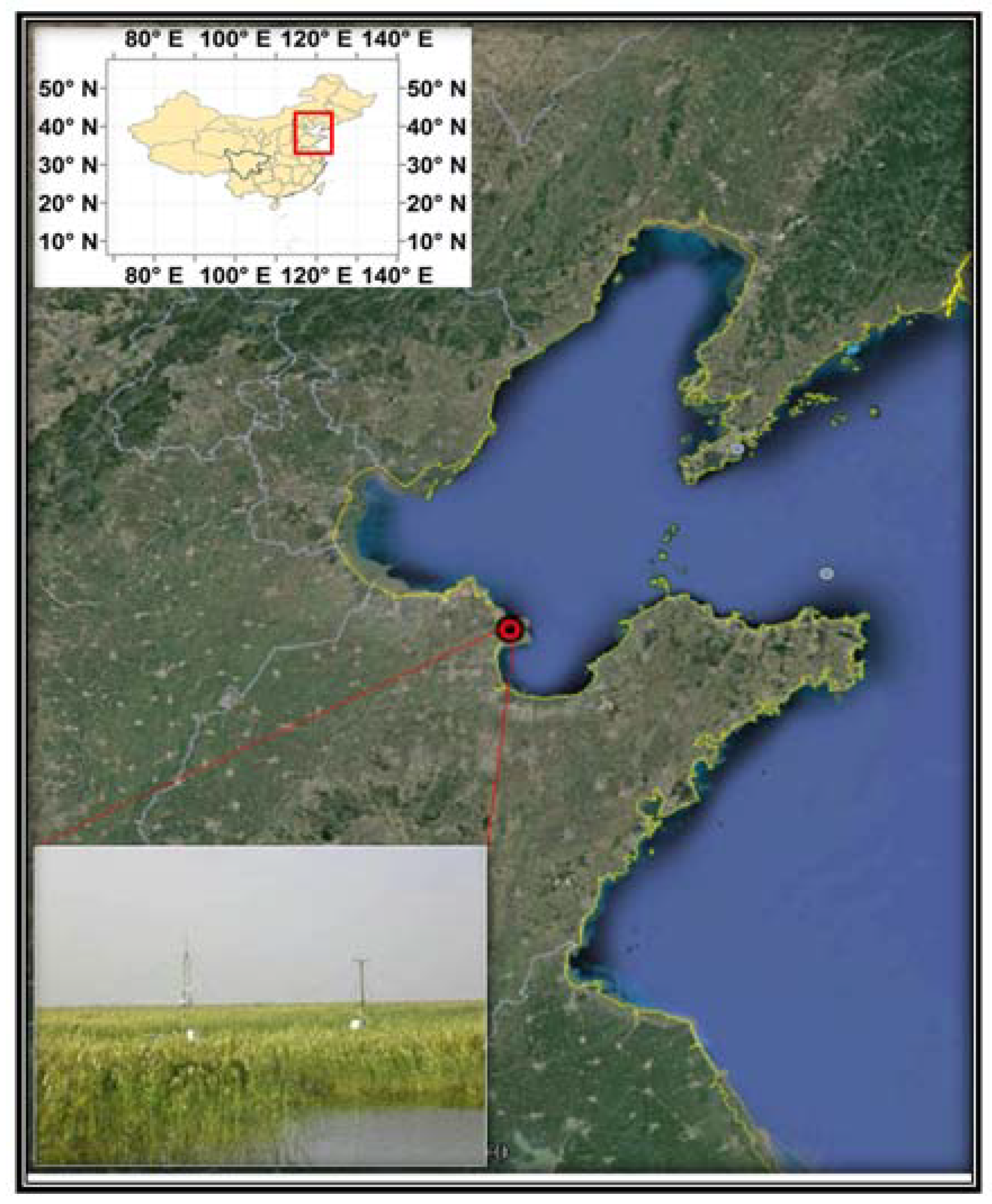
2.1. Description of the Study Region

Our study was carried out in the Yellow River Delta Nature Reserve (37°45′59″ N, 119°09′05″ E, −4 m above sea level; Figure 1). The nature reserve covers an area of 15.3 × 10⁴ ha. Our EC tower was established at the coastal zone of the Yellow River Delta Nature Reserve. In this region, the dominant wind direction is the north and northwest wind. The average annual wind speed is about 4 m/s. The annual mean air temperature is 12.1 °C [41,45]. The annual mean precipitation is 520 mm, which mainly concentrates in summer. The annual evaporation is 1962 mm and frost-free period is 196 days. The dominated soil type is coastal saline soil. The pH of the soil is 7.6–8.5. The dominant vegetation includes both the herbaceous plants (Phragmites australis and Suaeda salsa) and the shrub (Tamarix chinensis). The height of plants ranges from 120 to 200 cm.

2.2. CO₂ Flux and Climate Data from the Eddy Flux Tower Site

The EC instrument was established at the study site since 2008 (Figure 1), with the observation of CO₂ and water fluxes, wind speed, and wind direction. The EC tower equipped with an open path infrared CO₂/H₂O gas analyzer (Li 7500, LI-COR Inc., Lincoln, NE, USA) and ultrasonic anemometer (CSAT3, Campbell Scientific Inc., Jackson, MS, USA), which were installed 4.5 m above ground level. The sonic anemometer and the infrared CO₂/H₂O gas analyzer output were recorded at half-hour intervals by datalogger (CR5000, Campbell Scientific, Inc., Jackson, MS, USA), with high frequency of 10 Hz. Carbon and energy fluxes were calculated by using the half-hour covariance of vertical wind velocity and virtual temperature, water vapor density, and CO₂ density [15].

We also measured some environmental factors that were used for gap filling calculations nearby the eddy tower. Photosynthetically active radiation (PAR) was observed by LI-190SB sensors (LI-COR Inc., Lincoln, NE, USA). Relative humidity and air temperature were observed by humidity/temperature probes (HMP45C, VAISALA Woburn, MA, USA). Precipitation was measured at the height of 1.5 m above the ground level by a tipping bucket rain-gauge (TE525MM, Campbell Scientific, Inc., Jackson, MS, USA). The copper-constantan thermocouples were installed at five depths (0.05, 0.10, 0.20, 0.50, and 1.0 m) below the ground to measure soil temperature. All data were saved in the digital datalogger (CR23X; Campbell Scientific, Inc., Jackson, MS, USA) [19].

For reducing the measurement-induced uncertainties, quality control was conducted for the observed data during 2009–2010. The CO₂ flux data observed during rainfall or snowfall or instrument failure (e.g., system maintenance, power outages, etc.) were eliminated as invalid data that has led to data gaps. To fill the CO₂ flux data gap, the gap filling methods, including mean diurnal variation (MDV), of previous periods and nonlinear regression were used in this study. For the MDV method, the means for different time interval (window size, usually 4–15 days) that were based on adjacent days were used to replace the missing flux data. Nonlinear regression method was interpolated by establishing the regression relationships between net ecosystem CO₂ exchanges (NEE) components and the associated environmental factors during the studied period [46].

Generally, the EC measured C fluxes represent NEE, which is the balance between ecosystem respiration (R_e) and GPP [47]. Therefore, GPP can be obtained by the difference between R_e and NEE. R_e is summed by the daytime (R_e,day) and nighttime (R_e,night) ecosystem respiration. R_e,night is derived from the nighttime NEE. Because R_e,night is relevant to the soil temperature (T_s) [15,48], a temperature dependent model was derived from the observed R_e,night with T_s [19]. Then, we estimated the R_e,day rates and GPP by extrapolating the exponential relationship to the daytime periods.

$$GPP=R_e-NEE$$

(1)

$$R_e=R_{\mathrm{e},\mathrm{day}}+R_{\mathrm{e},\mathrm{night}}$$

(2)

$$R_{\mathrm{e},\mathrm{night}}=a{e}^{(bTs)}$$

(3)

where T_s is soil temperature (°C) at the depth of 0.05 m, and a and b are coefficients. During the data processing, the unit of CO₂ fluxes (NEE, GPP, R_e, R_e,day, R_e,night) is mg CO₂ m⁻² s⁻¹. After that, we accumulated and converted all data to the whole day, and obtained the daily CO₂ flux data, when the unit of CO₂ fluxes (NEE, GPP, R_e) is g CO₂ m⁻² day⁻¹ or g C m⁻² day⁻¹.

The daily GPP and climate data were aggregated to eight-day intervals in order to be consistent with MODIS eight-day composites. The aggregated eight-day GPP and climate data over 2009–2010 were utilized as parameter, input, and validated data in this study to support model simulation and validation.

2.3. Moderate Resolution Imaging Spectroradiometer Data and Vegetation Indices

The time series site-specific VIs for the targeted wetland EC tower were extracted from the MODIS datasets. We mainly used seven spectral bands to study vegetation and land surface: blue (459–479 nm), green (545–565 nm), red (620–670 nm), near infrared (NIR, 841–875 nm, 1230–1250 nm), and shortwave infrared (SWIR, 1628–1652 nm, 2105–2155 nm). In this study, based on the location (latitude and longitude) of the targeted EC tower, we downloaded the eight-day MOD09A1 data over 2009–2010 from Earth Observation and Modeling Facility (EOMF), the University of Oklahoma website (http://www.eomf.ou.edu). Then, we calculated EVI [37], LSWI [33], and NDVI [32] based on the reflectance values of the eight-day MODIS dataset from the blue, red, NIR, and SWIR spectral bands [33]. Owing to some defects of the NDVI, the EVI was proposed by using a feedback-based approach that incorporates both background adjustment and atmospheric resistance concepts into the NDVI, resulting in a feedback-based, soil and atmosphere resistant vegetation index [37]. Furthermore, VPM model used EVI and LSWI as important input data to simulate the dynamics of GPP at the targeted coastal wetland.

$$EVI=2.5\times \frac{{\rho }_{\mathrm{nir}}-{\rho }_{\mathrm{red}}}{{\rho }_{\mathrm{nir}}+(6\times {\rho }_{\mathrm{red}}-7.5\times {\rho }_{\mathrm{blue}})+1}$$

(4)

$$LSWI=\frac{{\rho }_{\mathrm{nir}}-{\rho }_{\mathrm{swir}}}{{\rho }_{\mathrm{nir}}+{\rho }_{\mathrm{swir}}}$$

(5)

$$NDVI=\frac{{\rho }_{\mathrm{nir}}-{\rho }_{\mathrm{red}}}{{\rho }_{\mathrm{nir}}+{\rho }_{\mathrm{red}}}$$

(6)

where ρ_blue, ρ_red, ρ_nir, and ρ_swir represent the surface reflectance values of blue, red, NIR, and SWIR bands, respectively [33,39,49].

For time series of VIs calculated from surface reflectance, a simple approach was employed to fill those cloudy pixels [36,50]. The gap-filling procedure that was employed for cloudy pixels of VIs was reported in the earlier studies [22,36,39]. A three-point time series filter X(t − 1), X(t), and X(t + 1)) was employed to correct a cloudy pixel using values of non-cloudy pixels in the window. If X(t + 1) and X(t − 1) pixels were cloud-free, the average of X(t +1) and X(t − 1) was calculated and was used as X(t). If only one pixel (either X(t + 1) or X(t − 1)) was cloud-free, then we used that pixel to substitute X(t). If the three-point time series filter was not available, then we expanded it to a five-point time series filter (X(t − 2), X(t − 1), X(t), X(t + 1), and X(t + 2)) [36]. The gap filling procedure was same as the above three-point time series filter.

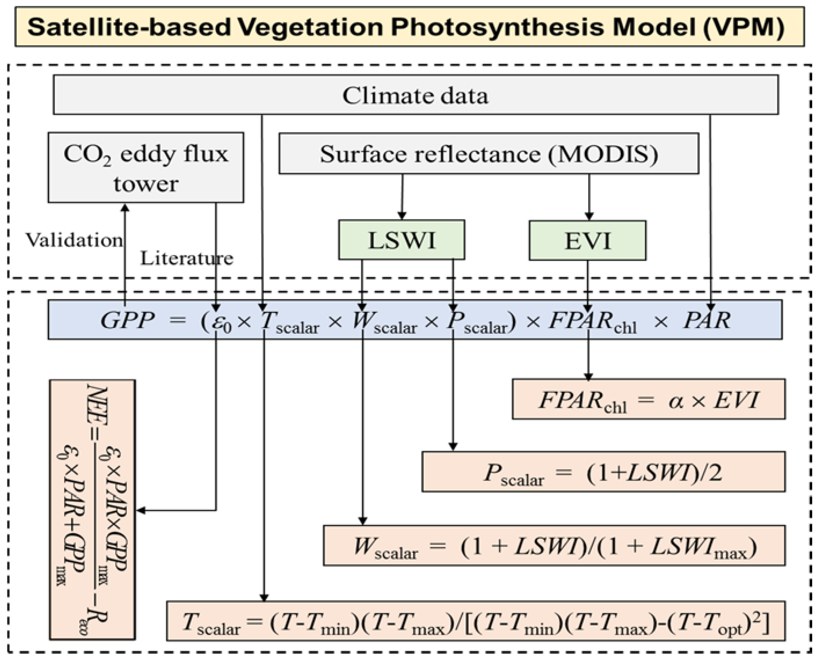
2.4. The Moderate Resolution Imaging Spectroradiometer-Based Vegetation Photosynthesis Model

2.4.1. Model Structure

As a RS-based vegetation photosynthesis model for simulating GPP [33], the VPM model is based on the conceptual partitioning of chlorophyll and non-photosynthetically active vegetation at the canopy. Air temperature (Ta), the EVI, LSWI, and PAR are the input data of the VPM model (Figure 2).

VPM estimates GPP over the photosynthetically active period of vegetation [33,36]:

$$GPP={\mathsf{\epsilon }}_{\mathrm{g}}\times FPA{R}_{\mathrm{chl}}\times PAR$$

(7)

where parameter ε_g is the light use efficiency (LUE) (μmol CO₂/μmol photosynthetic photon flux density, PPFD), which is affected by leaf phenology, temperature, and water; parameter PAR is the photosynthetically active radiation (μmol PPFD), and parameter FPAR_chl is the fraction of PAR absorbed by leaf chlorophyll in the canopy.

In the VPM model, FPAR_chl is calculated as [10,23,33,36,39,40]:

$$FPA{R}_{\mathrm{chl}}=\mathsf{\alpha }\times EVI$$

(8)

where EVI is the Enhanced Vegetation Index, which is calculated from the reflectance values of the eight-day MODIS dataset; α is the coefficient in the EVI-FPAR_chl linear function, which is set to be 1.0 [33,36].

ε_g is calculated by the maximum light use efficiency (LUE) ε₀ (μmol CO₂/μmol PPFD) and the scalars for the effects of temperature, water and leaf phenology on light use efficiency of vegetation.

$${\mathsf{\epsilon }}_{\mathrm{g}}={\mathsf{\epsilon }}_0\times T_{\mathrm{scalar}}\times W_{\mathrm{scalar}}\times P_{\mathrm{scalar}}$$

(9)

T_scalar is the scalar of temperature on photosynthesis, which is estimated by the Terrestrial Ecosystem Model (TEM) [51]; W_scalar is the impact of water on vegetation photosynthesis with LSWI_max [40]; and, P_scalar is the scalar for the impact of leaf phenology on photosynthesis within the canopy [39].

$$T_{scalar}=\frac{(T-T_{\min })(T-T_{\max })}{[(T-T_{\min })(T-T_{\max })]-{(T-T_{opt})}^2}$$

(10)

$$W_{scalar}=\frac{1+LSWI}{1+LSW{I}_{\max }}$$

(11)

$$P_{scalar}=\frac{1+LSWI}{2}$$

(12)

where LSWI_max is the maximum LSWI during 2009–2010 [15,26,27]; T_max, T_min, and T_opt are the maximum, minimum, and optimal air temperature during photosynthesis, respectively.

2.4.2. Model Parameterization

In order to normally run the VPM model for simulating GPP of coastal wetland using input data, such as climate observation and MODIS imagery, we conducted a series of model parameterization.

Different vegetation types have a different ε₀ value. It can be obtained from analysis of NEE and photosynthetic photon flux density of the EC tower site [52,53]. In this study, we used the Michaelis–Menten function (Equation (13)) in order to estimate the ε₀ of local vegetation type by the nonlinear model between the observed NEE and incident PAR, according to the flux data at 30 min intervals. Here, we took 2016.67 mg CO₂ mol⁻¹ PAR as ε₀ during the study period:

$$NEE=\frac{{\epsilon }_0\times PAR\times GP{P}_{\max }}{{\epsilon }_0\times PAR+GP{P}_{\max }}-R_{\mathrm{eco}}$$

(13)

where GPP_max (mg CO₂ m⁻² s⁻¹) is maximum gross primary production, R_eco (mg CO₂ m⁻² s⁻¹) is ecosystem respiration, NEE (mg CO₂ m⁻² s⁻¹) is the net ecosystem CO₂ exchange, PAR is the photosynthetically active radiation (μmol PPFD). Based on the diurnal GPP flux data, we chose the maximum value of GPP (0.63 mg CO₂ m⁻² s⁻¹) during the study period as GPP_max.

Different vegetation types have different estimation values of T_scalar, T_min, T_opt, and T_max [33]. The daily daytime mean temperature was calculated by using the daily maximum and minimum air temperature, rather than daily mean air temperature [33,54]. In our study, if the air temperature of the study site falls below T_min, T_scalar is set to zero. Because T_scalar is the scalar of temperature on plant photosynthesis activities, we consider the local meteorological conditions and plant growth (observed GPP) comprehensively. When considering the effect of low temperature on plant growth, we finally defined T_min as 0 °C (cold damage to plants). Based on the observed maximum temperature during the two study years, we finally defined T_max as 35 °C. We also defined site-specific T_opt as 26 °C by exploring the correlation between the observed vegetation indices, GPP and air temperature over 2009–2010.

W_scalar can be derived from the water-sensitive vegetation index LSWI and LSWI_max. Site-specific LSWI_max is estimated according to the time series MODIS data [26,33,36]. As a water-sensitive vegetation index, LSWI_max varies across years under different water condition. Using the observed eight-day MODIS reflectance data, we calculated the site-specific LSWI values over 2009–2010 and chose the maximum value during the growing season as LSWI_max (0.27 and 0.26 for 2009 and 2010, respectively).

2.4.3. Model Evaluation

In order to test VPM’s applicability for coastal wetland and to check the consistency between the modeled and the observed results, four statistical criteria were used for the model evaluation: (i) the coefficient of determination (R²). Due to temporal autocorrelation within simulated GPP and EC-based GPP, generalized least square regression was conducted by using gls() function in R package nlme to adjust the residuals. Accordingly, the R²_{Cox and Snell} was instead used as pseudo-R² by performing nagelkerke() function in package rcompanion; Equation (2), the root of mean square error (RMSE, Equation (14)); Equation (3), the relative mean deviation (RMD, Equation (15)); Equation (4), the relative error (RE) [55]. The RMSE provides the prediction error of model by heavily weighting high errors. The RMD can smooth out the differences between the simulated and measured results by weighting all of the errors in the same way, which when close to 0 indicate the absence of bias for the model [15,56]. We use SPSS version 20.0 (SPSS Inc., Chicago, IL, USA) and R package 3.2.1 [57] to conduct all of the statistical calculations.

$$RMSE=\frac{100}{\overline{O}}\sqrt{\frac{{\displaystyle {\sum }_{i=1}^n{(P_i-O_i)}^2}}{n}}$$

(14)

$$RMD=\frac{100}{\overline{O}}{\displaystyle {\sum }_{i=1}^n\frac{P_i-O_i}{n}}$$

(15)

where O_i represent the EC estimated values and P_i represent the model-simulated values. $\overline{O}$ is the mean of the EC estimated value and $\overline{P}$ is the mean of the model-predicted value. n is the number of observations.

3. Results

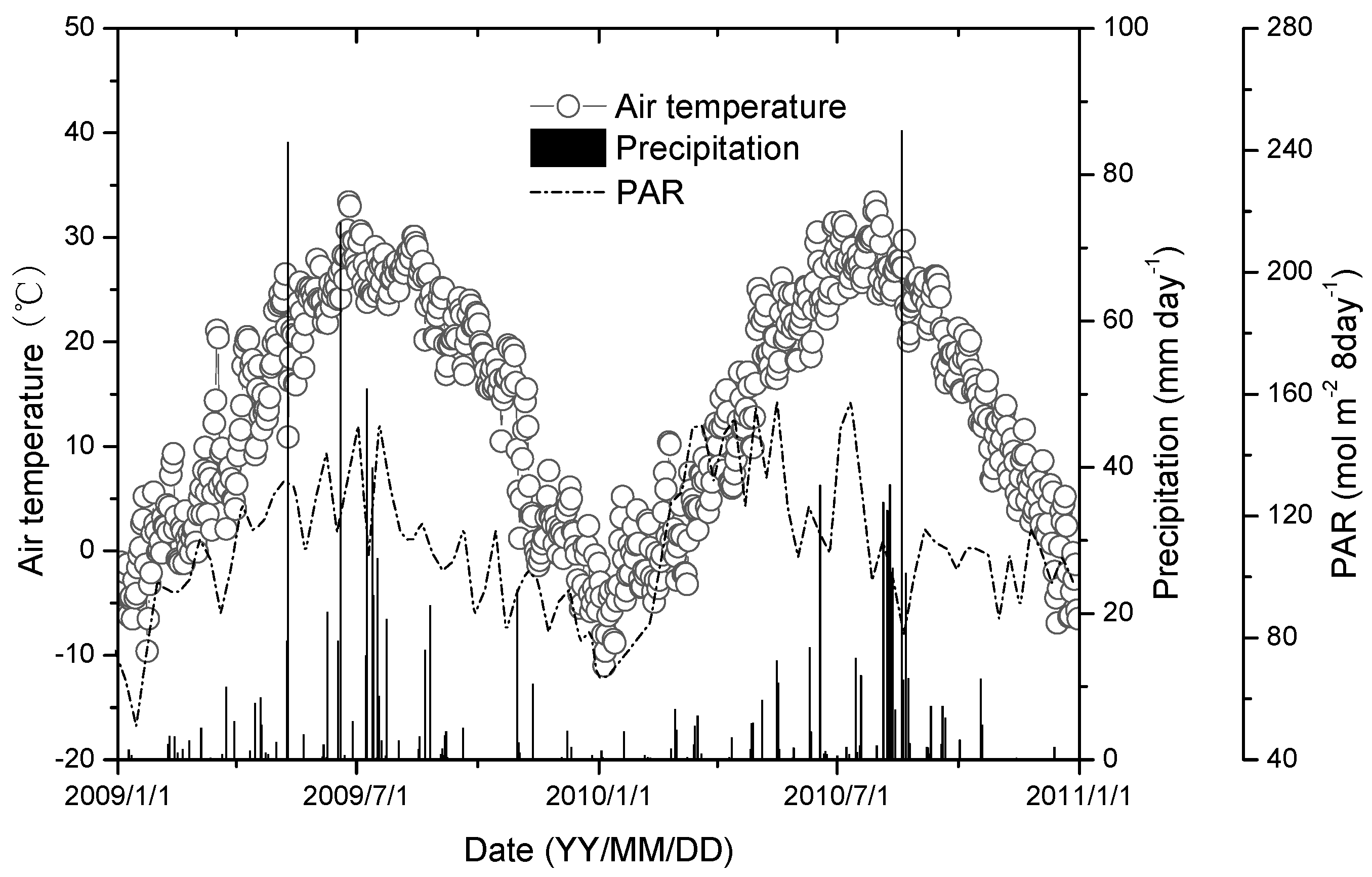
3.1. Seasonal Dynamics of Hydrothermal Conditions, Vegetation Indices, and Gross Primary Production

The dynamics of the main meteorological variables are given in Figure 3. There was significant seasonal variation of daily air temperature (Ta) during 2009–2010, varying between −11.0 and 33.4 °C. The maximum and minimum values of Ta were found during July and January, respectively. But, no strong inter-annual difference among the different temperature regimes was found. The mean annual Ta were 13.9 and 13.3 °C in 2009 and 2010, respectively, both warmer than the long-term average (12.1 °C). The annual precipitation (rainfall and snowfall), measured at the tower in the experiment were 571.4 and 523.5 mm for 2009 and 2010, respectively, both higher than the long-term average (520.0 mm). In 2009, there were 68 days with precipitation. In 2010, there were 66 days with precipitation (Figure 3). The results also show that the rainy season started in early June, and it ended in late August.

The EVI, NDVI, and LSWI curves can better demonstrate the development and the senescence of coastal wetland vegetation (Figure 4a–c). Both time series EVI and NDVI from 2009 to 2010 showed a strong seasonality for this coastal wetland ecosystem. They increased in spring and peaked in mid-August (21 August), and then declined and kept low in winter, corresponding well with the seasonal dynamics of GPP_EC (Figure 4). However, seasonal variation in EVI within the growing seasons differed slightly with the NDVI in terms of phase and magnitude (Figure 4a,b). The values of NDVI were obviously higher than that of EVI from late March to early November in both years. The maximum values of EVI (0.21 and 0.32) were much lower than the peaks of NDVI (0.40 and 0.61) in 2009 and 2010, respectively. The LSWI also exhibited seasonal variation, but it did not vary with time as significantly, as did NDVI or EVI, especially during plant growing season (Figure 4c). As shown in Figure 4c, the peak LSWI values were 0.27 (28 July) and 0.26 (12 August) for 2009 and 2010, respectively, advancing about 8–24 days as compared with the peak values of NDVI and EVI. High EVI and LSWI in August indicated that the canopy was rapidly developed photosynthetically active, while the quick drop of both EVI and LSWI in late September indicated an early plant senescence (Figure 4).

The time series GPP_EC also shows an obviously seasonal and inter-annual variability (Figure 4d). With the raise of Ta and PAR, the photosynthetic capacity of coastal wetland ecosystem gradually increased. GPP_EC began to increase in mid-April (1 g C m⁻² day⁻¹ or higher), achieved the maximum values in early August (2009) or mid-July (2010), and it then decreased to below 1 g C m⁻² day⁻¹ in late October (2009) or early November (2010). The peak and annual values of GPP_EC in 2009 were 9.05 g C m⁻² and 1068.51 g C m⁻², respectively; whereas, the respective values of GPP_EC in 2010 were 9.88 g C m⁻² and 1102.84 g C m⁻², respectively (Figure 4d). The C uptake period (CUP) of wetland plant, as defined by GPP_EC > 1 g C m⁻² day⁻¹, ranges from mid-April to early November, which can be partly explained by the variation of Ta and PAR (Figure 3 and Figure 4d). Further, the growing season period for coastal wetland vegetation, as defined by Vis, agreed with the CUP defined by GPP_EC over the two study years (Figure 4d).

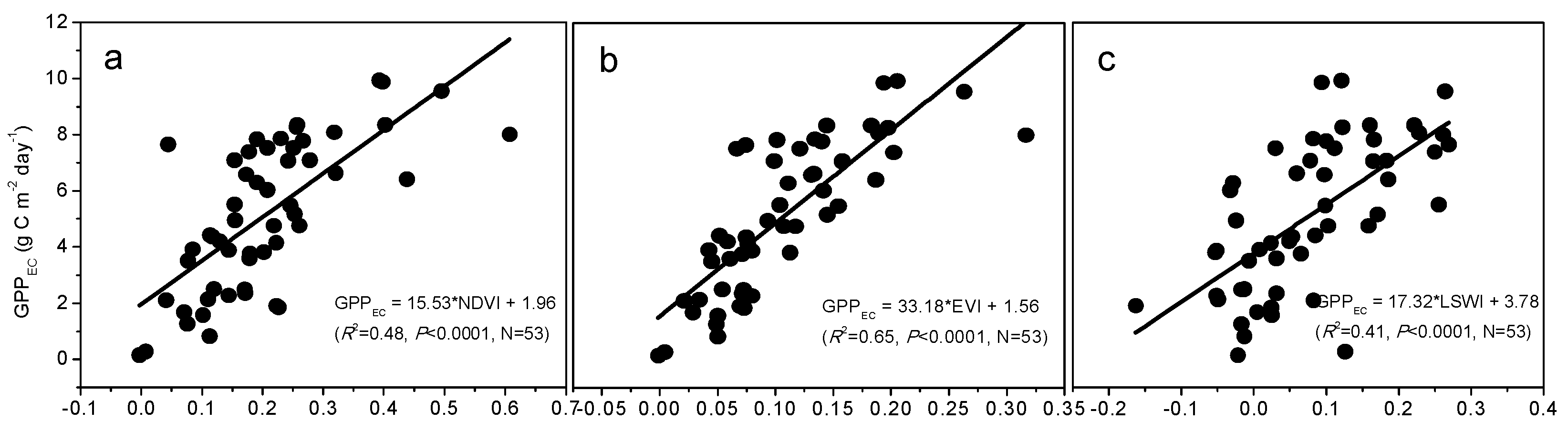
3.2. Correlation between GPP_EC, Vegetation Indices, and Air Temperature

The comparisons between GPP_EC and VIs (EVI and NDVI) show that EVI has a better relationship with GPP in terms of the phase and amplitude (Figure 4). In order to further evaluate the biological significance of VIs in GPP predictions, the simple linear relationships between GPP_EC and VIs were investigated (Figure 5). Correlation analyses show that the dynamics of GPP_EC correlated well with that of the VIs (EVI, NDVI, and LSWI), both in 2009 and 2010 (Figure 5). However, EVI (R² = 0.65, p < 0.0001) has a better correlation with GPP_EC than NDVI does (R² = 0.48, p < 0.0001). EVI can account for 65% of the variance in GPP_EC, while NDVI only 48%. Above results indirectly prove that the improved vegetation index EVI has a higher predictive power to simulate the GPP of the coastal wetland ecosystem. The LSWI also has a strong relationship with GPP_EC (R² = 0.41, p < 0.0001, Figure 5), showing that the land surface water content is important for the estimation of GPP during growing season.

We also analyzed the relationships between VIs (EVI, NDVI, and LSWI), GPP_EC, and air temperature (Ta). The regression analysis shows that Ta was positively correlated with NDVI (R² = 0.55, p < 0.0001), EVI (R² = 0.62, p < 0.0001), and GPP_EC (R² = 0.78, p < 0.0001), respectively (Figure 6a,b,d). NDVI, EVI, and GPP_EC gradually increased as the temperature rose, and the temporal variation in NDVI, EVI, and GPP_EC fluxes could be largely explained by air temperature. LSWI had a significant U-shaped relationship (R² = 0.28, p < 0.01) with air temperature. As temperature rose, LSWI decreased first, reached its bottom, and then increased. The demarcation point is about 10 °C (Figure 6c).

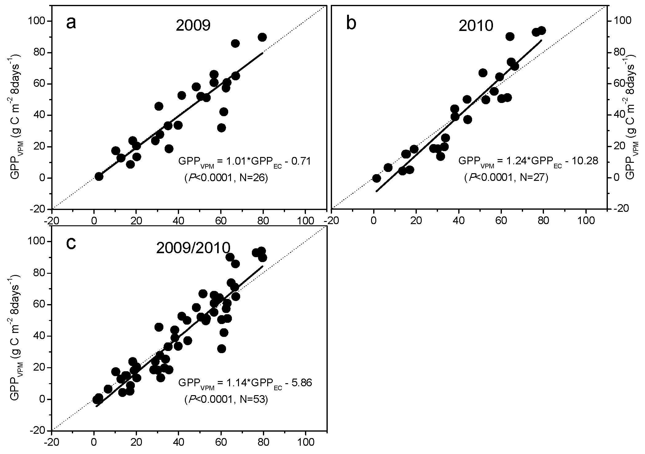
3.3. Simulation and Evaluation of Vegetation Photosynthesis Model

We run the VPM model based on the observation of Ta, PAR, and MODIS VIs (EVI and LSWI), and examined the seasonal variation of the modeled GPP (GPP_VPM) for the tested coastal wetland during 2009–2010 (Figure 7). GPP_VPM was close to zero from November to early March, then began to increase rapidly in mid-March, and achieved a peak in early-August and mid-July in 2009 and 2010, respectively. GPP_VPM declined gradually after reaching peak it and dropped below 1 g C m⁻² day⁻¹ by early-November. Comparisons between GPP_VPM and GPP_EC fluxes at eight-day time intervals show that the simulated eight-day GPP_VPM fluxes were in good agreement with GPP_EC fluxes regarding to the patterns and magnitudes. VPM fairly reappeared the U-shaped growth pattern, which driveled by the variation in Ta and PAR, and accurately simulated the seasonal dynamics of GPP_EC fluxes for the simulated two years. However, eight-day GPP_VPM peak values were slightly higher than GPP_EC in both 2009 and 2010 (Figure 7).

To further evaluate the accuracy of model simulation, a linear regression analysis between GPP_VPM and GPP_EC was conducted (Figure 8). For both years, the linear regression of GPP_VPM against GPP_EC shows a good correlation (R² ≥ 0.72, p < 0.0001; Figure 8;

Table 1. The evaluation of model simulation results in the typical coastal wetland. Four statistical criteria for the validation tests: pseudo-R², the coefficient of determination; RMSE, the root of mean square error; RMD, the relative mean deviation; and, RE, the relative error.

Items	Year	pseudo-R2	RMSE (%)	RMD (%)	GPPEC a (g C m−2)	GPPVPM a (g C m−2)	RE a	N
GPPVPM vs. GPPEC	2009	0.72 ***	25.09	−1.02	1068.51	1057.64	−1%	26
	2010	0.80 ***	25.47	−1.00	1102.84	1091.76	−1%	27
	2009–2010	0.73 ***	25.29	−1.01	2171.35	2149.39	−1%	53

*** Significant at probability levels of 0.0001. ^a Abbreviations: GPP, gross primary production; GPP_EC, estimated GPP from FLUX tower data; GPP_VPM, simulated GPP by VPM; RE (relative error) = [(GPP_VPM − GPP_EC)/GPP_EC] × 100%.

). The RMD and RMSE values were −1.01% and 25.29% during 2009–2010, respectively. The simulated annual GPP_VPM were 1057.64 and 1091.76 g C m⁻² yr⁻¹ for 2009 and 2010, respectively, which is slightly lower than the estimated annual GPP_EC (1068.51 and 1102.84 g C m⁻² yr⁻¹ for 2009 and 2010, respectively), both with relative error (RE) values of −1% (Table 1). Moreover, cumulative GPP fluxes simulated over the two years were in good agreement with the estimated values, with −1% RE (Table 1).

4. Discussion

4.1. Biophysical Performance of Vegetation Indices in Typical Coastal Wetland

Monitoring vegetation change over time at larger scales using vegetation indices has greatly enhanced our understanding of the changing environment [58,59]. Different vegetation indices vary in their biophysical expression and they can offer distinct information for the leaf phenological cycle, which in turn, affect plant photosynthesis and regulate ecosystem carbon balance [10,22,36]. Some researchers have reported that time series of NDVI, EVI (greenness-related vegetation indices), and LSWI (water-related vegetation index) can be used to delineate the green-up and the senescence phase at the canopy level [36,60]. However, which is the best vegetation index for the model to more accurately predict the plant production in coastal wetlands remains unknown. Therefore, it is important to evaluate the biophysical and phenological expression of different vegetation indices in coastal wetland ecosystems to accurately assess vegetation phenology and predict plant production [61,62].

In this study, we examined the relationship between NDVI, EVI, LSWI, and estimated GPP_EC, Ta, and evaluated the biophysical expression of vegetation indices in a typical coastal wetland. Both EVI and NDVI have significant correlations with GPP_EC, but EVI has a stronger correlation with GPP_EC, and hence has more biological and phenological significance in GPP predictions than the NDVI in this coastal wetland (Figure 5 and Figure 6). EVI can minimize the influences of soil condition and atmosphere in reflectance data by incorporating soil adjustment and atmospheric resistance factors [58]. Time series of LSWI also provide valuable information (e.g., water status) for simulating plant growth and wetland carbon exchange, even though it has a lower relationship between Ta and GPP_EC. It has a great potential in obtaining the water content information of leaf and canopy, and can more accurately identify the vegetation phenology by combining both NIR and SWIR bands [22,63,64]. The results in this study are consistent with earlier studies [10,15,22,23,33,40,65,66], in which all indirectly prove the hypothesis of chlorophyll-FPAR_chl-EVI and leaf 1 water-LSWI, as applied in the VPM model. However, it is necessary to further develop the LSWI-based phenology algorithm in the near future [40].

4.2. Model Comparison and Error Source Analysis

Recently, using the LUE models to simulate GPP plays an important role in the global carbon budget research, but our understanding of relative advantages and disadvantages of different models is still limited [67]. The VPM model simulated the trends of the coastal wetland phenology well and precisely predicted GPP (R² = 0.73) in this study. The MODIS-Photosynthesis (PSN) model also can simulate the global GPP and generate the Terra/MODIS GPP project (MOD17A2) [40,68]. Here, eight-day MODIS GPP product (GPP_MOD17A2) data during 2009–2010 were downloaded from the Oak Ridge National Laboratory’s Distributed Active Archive Center (DAAC) website (http://daac.ornl.gov/MODIS) [69,70]. Then, we compared the differences between GPP_EC, GPP_VPM, and GPP_MOD17A2 in our studied coastal wetland. A Taylor diagram was also used to display the quality of model predictions against the observations [71]. We found that both GPP_EC and GPP_VPM were substantially higher than GPP_MOD17A2 in terms of the magnitudes. The underestimated range of GPP_MOD17A2 is probably 40–80% (see Figure 9). Some previous studies also reported that the MODIS-PSN model underestimated GPP in different ecosystems [15,40,72,73,74]. However, Jin et al., found that GPP_MOD17A2 was significantly lower than GPP_EC during the prophase of the growing season, but higher than GPP_EC during the late growing season at broadleaf deciduous woodland [39].

The discrepancies between GPP_MOD17A2 and GPP_EC may result from two underestimated sources. First, GPP_MOD17A2 uses global meteorological reanalysis dataset, including average and minimum Ta, incident PAR, and specific humidity. The input weather data of MODIS-PSN model may not match the local air temperature data. The second source is the parameter ofε₀ in MODIS-PSN [66,75]. ε₀ is a very important parameter in the PEM models to estimate GPP and differs significantly among vegetation types [76]. However, the ε₀ and some other biome-specific physiological parameters are not differentiated from the different performance of a specific biome [77]. The EC technique provides an appropriate method to accurately estimate the parameter ε₀ by using a large number of measured data [23,30]. In this study, we estimated the ε₀ value by fitting the nonlinear model between observed NEE and PAR in 2009 and 2010. Then, we used the site-specific climate data, the individual ε₀ estimated from CO₂ flux data, and vegetation indices (EVI, LSWI) as input data and the parameters of VPM to simulate the GPP dynamics of coastal wetland. Therefore, future works should pay more attention to the local climate data and biome-specific physiological parameters in using GPP_MOD17A2 for regional analysis.

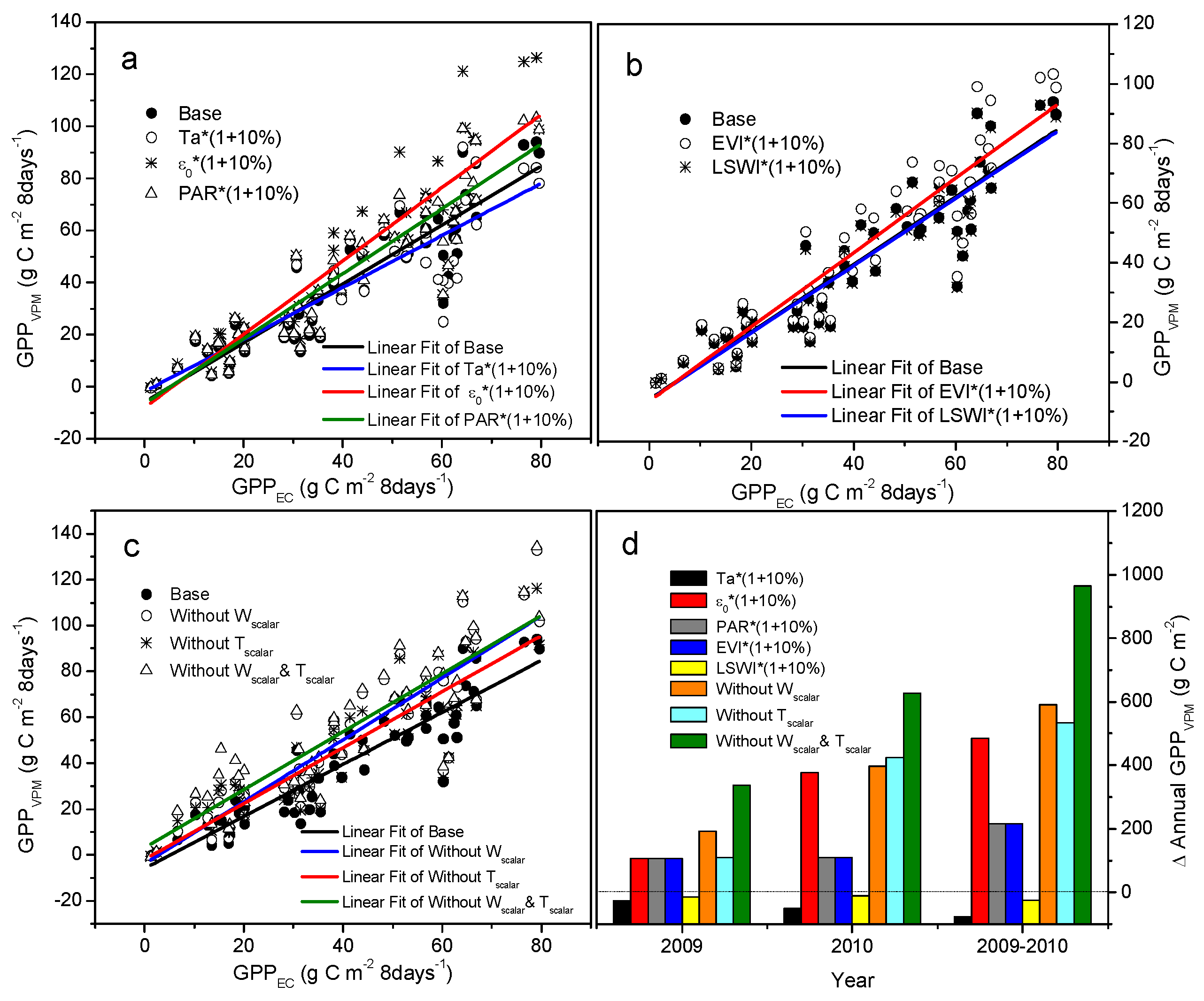
4.3. Sensitivity and Uncertainty for Vegetation Photosynthesis Model Simulations

In general, there are always some errors in model simulations. The analysis of sources and uncertainties for the errors are very important for future improvement and the development of these models [78,79]. In this study, the VPM simulation results show that the VPM model can correctly simulate the seasonal variations of GPP. The modeled results can explain about 85% of GPP_EC changes over the two study years. However, there still exist some differences between seasonal GPP_VPM and GPP_EC in this study, such as higher GPP_VPM from late July to early August in 2009 and 2010, and lower GPP_VPM in late May in 2010 (Figure 7). The discrepancies between GPP_EC and GPP_VPM can be attributed, in part, to the estimation error of tower-based GPP_EC [36,80]. GPP_EC is calculated as the difference between ecosystem respiration and NEE [15,36]. The estimation error of daytime ecosystem respiration, which is the difference between ecosystem respiration and observed nighttime ecosystem respiration, may lead to the error of estimation (either overestimation or underestimation) of GPP_EC [15,36,39,40].

Another error source may be attributed to the modeling of GPP_VPM from VPM [33]. To further clarify the sources and uncertainty of the GPP_VPM errors, we conducted a sensitivity analysis for some parameters and variables of the model (Figure 10). The alternative sensitivity scenarios of input parameter were set by increasing Ta, ε₀, PAR, EVI, and LSWI by 10%, respectively. When compared with the base scenario, the sensitivity of ε₀ and PAR are relatively larger than that of Ta in this coastal wetland (Figure 10a,d). The potential conversion efficiency of absorbed photosynthetically active radiation is largely determined by ε₀, which varies with vegetation types and study regions [23,39], and it may even affect the accuracy of GPP simulation [40,81]. PAR is an important variable in the GPP simulation, lower/higher PAR values may result in the under/over-estimation of GPP for the assumed relationship between GPP and PAR in VPM model [15,82]. Therefore, the accurate estimation of ε₀ and development of PAR observation would substantially improve the simulated accuracy of the VPM model and other models [36]. The source of uncertainty also come from the MODIS time series vegetation indices, such as the effects of cloud, cloud shadow, aerosols, and other atmospheric condition [40]. The EVI is more sensitive than LSWI to GPP simulation during 2009–2010 in this typical coastal wetland (Figure 10b,d). Future work should focus on how to avoid and mitigate the effects of angular geometry on surface albedo and to reconstruct the time series data of vegetation indices in order to improve the accuracy of vegetation indices, especially EVI.

The simulation uncertainties of VPM also come from two intermediate variables that are related to water (W_scalar) and temperature (T_scalar) [39]. We use the two intermediate variables to set three sensitivity scenarios, including without T_scalar (ε_g = W_scalar × P_scalar × ε₀), without W_scalar (ε_g = T_scalar × P_scalar × ε₀), and without T_scalar & W_scalar (ε_g = P_scalar × ε₀). When there is no T_scalar in the VPM, the model overestimated GPP by about 10%, 39%, and 25% in 2009, 2010, and 2009–2010, respectively. In the absence of W_scalar in VPM, the model overestimated GPP by about 18%, 36%, and 27% in 2009, 2010, and 2009–2010, respectively. When there is no both T_scalar and W_scalar in VPM, the model overestimated GPP by about 31%, 57%, and 44% in 2009, 2010, and 2009–2010, respectively (Figure 10c,d). Above results indicated that both T_scalar and W_scalar have profound effects on the predicted accuracy of GPP. It will be essential to integrate both temperature and water to downscale maximum light use efficiency to better represent the impacts of temperature and water on plant photosynthesis and GPP [36,39,40,66].

5. Conclusions

In this study, we incorporated climate and remote sensing data into a satellite-based VPM model to investigate the biophysical performance of different vegetation indices and to evaluate the applicability and accuracy of the VPM model for simulating GPP of coastal wetland in China. The results indicated that air temperature can explain most of the seasonal variation in vegetation indices and GPP_EC fluxes. Time series of greenness-related EVI and water-related LSWI can better delineate the green-up and senescence phases of coastal wetland vegetation, which are in accordance with the CUP, as defined by GPP_EC. Further, both EVI and water-sensitive LSWI have higher predictive power for simulating the GPP in this coastal wetland. The EVI-based VPM model is able to simulate the U-shaped growth pattern of the coastal plant and accurately simulate the trajectories of the seasonal dynamics of GPP_EC fluxes, explaining about 85% of GPP_EC changes. Further development and improvement of VPM for nearby coastal wetlands and the spatial-temporal scale expansion are necessary for regional and continental simulations of GPP in the future.

References

1. Choi, Y.; Wang, Y.; Hsieh, Y.P.; Robinson, L. Vegetation succession and carbon sequestration in a coastal wetland in northwest Florida: Evidence from carbon isotopes. Glob. Chang. Biol. 2001, 15, 311–319. [Google Scholar] [CrossRef]
2. Cicin-Sain, B.; Knecht, R.W.; Jang, D.; Fisk, G.W. Integrated Coastal and Ocean Management: Concepts and Practices; Island Press: Washington, DC, USA, 1998; p. 471. ISBN 978-1559636049. [Google Scholar]
3. Titus, J. Greenhouse effect and coastal wetland policy: How Americans could abandon an area the size of Massachusetts at minimum cost. Environ. Manag. 1991, 15, 39–58. [Google Scholar] [CrossRef]
4. Yanez-Arancibia, A. Terms of reference towards coastal management and sustainable development in Latin America: Introduction to Special Issue on progress and experiences. Ocean Coast. Manag. 1999, 42, 77–104. [Google Scholar]
5. Yan, Y.; Zhao, B.; Chen, J.; Guo, H.; Gu, Y.; Wu, Q.; Li, B. Closing the carbon budget of estuarine wetlands with tower-based measurements and MODIS time series. Glob. Chang. Biol. 2008, 14, 1690–1702. [Google Scholar] [CrossRef]
6. Ye, S.; Laws, E.A.; Yuknis, N.; Ding, X.; Yuan, H.; Zhao, G.; Wang, J.; Yu, X.; Pei, S.; DeLaune, R.D. Carbon sequestration and soil accretion in coastal wetland communities of the Yellow River Delta and Liaohe Delta, China. Estuar. Coast. 2015, 38, 1885–1897. [Google Scholar] [CrossRef]
7. Chen, J.; Zhang, H.; Liu, Z.; Che, M.; Chen, B. Evaluating parameter adjustment in the MODIS gross primary production algorithm based on eddy covariance tower measurements. Remote Sens. 2014, 6, 3321–3348. [Google Scholar] [CrossRef]
8. Running, S.W.; Nemani, R.R.; Heinsch, F.A.; Zhao, M.S.; Reeves, M.; Hashimoto, H. A continuous satellite-derived measure of global terrestrial primary production. Bioscience 2004, 54, 547–560. [Google Scholar] [CrossRef]
9. Tao, F.; Yokozawa, M.; Zhang, Z.; Xu, Y.; Hayashi, Y. Remote sensing of crop production in China by production efficiency models: Models comparisons, estimates and uncertainties. Ecol. Model. 2005, 183, 385–396. [Google Scholar] [CrossRef]
10. Yan, H.M.; Fu, Y.L.; Xiao, X.M.; Huang, H.Q.; He, H.L.; Ediger, L. Modeling gross primary productivity for winter wheat-maize double cropping system using MODIS time series and CO2 eddy flux tower data. Agric. Ecosyst. Environ. 2009, 129, 391–400. [Google Scholar] [CrossRef]
11. Campbell, J.E.; Berry, J.A.; Seibt, U. Large historical growth in global terrestrial gross primary production. Nature 2017, 544, 84–87. [Google Scholar] [CrossRef] [PubMed]
12. Stagg, C.L.; Schoolmaster, D.R.; Piazza, S.C. A landscape-scale assessment of above-and belowground primary production in coastal wetlands: Implications for climate change-induced community shifts. Estuar. Coast. 2017, 40, 856–879. [Google Scholar] [CrossRef]
13. Liu, Z.; Wang, L.; Wang, S. Comparison of different GPP models in China using MODIS image and ChinaFLUX data. Remote Sens. 2014, 6, 10215–10231. [Google Scholar] [CrossRef]
14. Baldocchi, D.; Falge, E.; Gu, L.H. FLUXNET: A new tool to study the temporal and spatial variability of ecosystem-scale carbon dioxide, water vapor, and energy flux densities. Bull. Am. Meteorol. Soc. 2001, 82, 2415–2434. [Google Scholar] [CrossRef]
15. Kang, X.M.; Wang, Y.F.; Chen, H.; Tian, J.Q.; Cui, X.Y.; Rui, Y.C.; Zhong, L.; Kardol, P.; Hao, Y.B.; Xiao, X.M. Modeling carbon fluxes using multi-temporal MODIS imagery and CO2 eddy flux tower data in Zoige Alpine Wetland, South-West China. Wetlands 2014, 34, 603–618. [Google Scholar] [CrossRef]
16. Leuning, R.; Cleugh, H.A.; Zegelin, S.J.; Hughes, D. Carbon and water fluxes over a temperate Eucalyptus forest and a tropical wet/dry savanna in Australia: Measurements and comparison with MODIS remote sensing estimates. Agric. For. Meteorol. 2005, 129, 151–173. [Google Scholar] [CrossRef]
17. Wang, Y.F.; Cui, X.Y.; Hao, Y.B.; Mei, X.R.; Yu, G.Y.; Huang, X.Z.; Kang, X.M.; Zhou, X.Q. The fluxes of CO2 from grazed and fenced temperate steppe during two drought years on the Inner Mongolia Plateau, China. Sci. Total Environ. 2011, 410, 182–190. [Google Scholar] [CrossRef] [PubMed]
18. Baldocchi, D.D. Assessing the eddy covariance technique for evaluating carbon dioxide exchange rates of ecosystems: Past, present and future. Glob. Chang. Biol. 2003, 9, 479–492. [Google Scholar] [CrossRef]
19. Kang, X.M.; Hao, Y.B.; Li, C.S.; Cui, X.Y.; Wang, J.Z.; Rui, Y.C.; Niu, H.S.; Wang, Y.F. Modeling impacts of climate change on carbon dynamics in a steppe ecosystem in Inner Mongolia, China. J. Soil. Sediment. 2011, 11, 562–576. [Google Scholar] [CrossRef]
20. Song, C.; Sun, L.; Huang, Y. Carbon exchange in a freshwater marsh in the Sanjiang Plain, Northeastern China. Agric. For. Meteorol. 2011, 151, 1131–1138. [Google Scholar] [CrossRef]
21. Belshe, E.; Schuur, E.; Bolker, B.; Bracho, R. Incorporating spatial heterogeneity created by permafrost thaw into a landscape carbon estimate. J. Geophys. Res. 2012, 117, G01026. [Google Scholar] [CrossRef]
22. Kang, X.M.; Hao, Y.B.; Cui, X.Y.; Chen, H.; Huang, S.X.; Du, Y.G.; Li, W.; Kardol, P.; Xiao, X.M.; Cui, L.J. Variability and changes in climate, phenology, and gross primary production of an alpine wetland ecosystem. Remote Sens. 2016, 8, 391. [Google Scholar] [CrossRef]
23. Li, Z.Q.; Yu, G.R.; Xiao, X.M.; Li, Y.N.; Zhao, X.Q.; Ren, C.Y.; Zhang, L.M.; Fu, Y.L. Modeling gross primary production of alpine ecosystems in the Tibetan Plateau using MODIS images and climate data. Remote Sens. Environ. 2007, 107, 510–519. [Google Scholar] [CrossRef]
24. Malhi, Y. The productivity, metabolism and carbon cycle of tropical forest vegetation. J. Ecol. 2012, 100, 65–75. [Google Scholar] [CrossRef]
25. Knox, S.H.; Dronova, I.; Sturtevant, C. Using digital camera and Landsat imagery with eddy covariance data to model gross primary production in restored wetlands. Agric. For. Meteorol. 2017, 237, 233–245. [Google Scholar] [CrossRef]
26. Gamon, J.A.; Huemmrich, K.F.; Stone, R.S.; Tweedie, C.E. Spatial and temporal variation in primary productivity (NDVI) of coastal Alaskan tundra: Decreased vegetation growth following earlier snowmelt. Remote Sens. Environ. 2013, 129, 144–153. [Google Scholar] [CrossRef]
27. Zhang, A.Z.; Jia, G.S. Monitoring meteorological drought in semiarid regions using multi-sensor microwave remote sensing data. Remote Sens. Environ. 2013, 134, 12–23. [Google Scholar] [CrossRef]
28. Machwitz, M.; Gessner, U.; Conrad, C.; Falk, U.; Richters, J.; Dech, S. Modelling the gross primary productivity of West Africa with the Regional Biomass Model RBM plus, using optimized 250 m MODIS FPAR and fractional vegetation cover information. Int. J. Appl. Earth Obs. Geoinf. 2015, 43, 177–194. [Google Scholar] [CrossRef]
29. Potter, C.S.; Randerson, J.T.; Field, C.B.; Matson, P.A.; Vitousek, P.M.; Mooney, H.A.; Klooster, S.A. Terrestrial ecosystem production—A process model-based on global satellite and surface data. Glob. Biogeochem. Cycle 1993, 7, 811–841. [Google Scholar] [CrossRef]
30. Turner, D.P.; Ritts, W.D.; Cohen, W.B.; Gower, S.T.; Zhao, M.S.; Running, S.W.; Wofsy, S.C.; Urbanski, S.; Dunn, A.L.; Munger, J.W. Scaling gross primary production (GPP) over boreal and deciduous forest landscapes in support of MODIS GPP product validation. Remote Sens. Environ. 2003, 88, 256–270. [Google Scholar] [CrossRef]
31. Yuan, W.P.; Liu, S.; Zhou, G.S.; Zhou, G.Y.; Tieszen, L.L.; Baldocchi, D.; Bernhofer, C.; Gholz, H.; Goldstein, A.H.; Goulden, M.L.; et al. Deriving a light use efficiency model from eddy covariance flux data for predicting daily gross primary production across biomes. Agric. For. Meteorol. 2007, 143, 189–207. [Google Scholar] [CrossRef]
32. Tucker, C.J. Red and photographic infrared linear combinations for monitoring vegetation. Remote Sens. Environ. 1979, 8, 127–150. [Google Scholar] [CrossRef]
33. Xiao, X.M.; Hollinger, D.; Aber, J.; Goltz, M.; Davidson, E.A.; Zhang, Q.Y.; Moore, B. Satellite-based modeling of gross primary production in an evergreen needleleaf forest. Remote Sens. Environ. 2004, 89, 519–534. [Google Scholar] [CrossRef]
34. Xiao, X.; Zhang, Q.; Hollinger, D.; Aber, J.; Moore, B. Modeling gross primary production of an everygreen needleleaf forest using satellite images and climate data. Ecol. Appl. 2005, 15, 954–969. [Google Scholar] [CrossRef]
35. Xiao, X.; Zhang, Q.; Saleska, S. Satellite-based modeling of gross primary production in a seasonally moist tropical evergreen forest. Remote Sens. Environ. 2005, 94, 105–122. [Google Scholar] [CrossRef]
36. Xiao, X.M.; Zhang, Q.; Braswell, B.; Urbanski, S.; Boles, S.; Wofsy, S.; Moore, B.; Ojima, D. Modeling gross primary production of temperate deciduous broadleaf forest using satellite images and climate data. Remote Sens. Environ. 2004, 91, 256–270. [Google Scholar] [CrossRef]
37. Huete, A.R.; Liu, H.Q.; Batchily, K.; van Leeuwen, W. A comparison of vegetation indices over a global set of TM images for EOS-MODIS. Remote Sens. Environ. 1997, 59, 440–451. [Google Scholar] [CrossRef]
38. Christian, B.; Joshi, N.; Saini, M. Seasonal variations in phenology and productivity of a tropical dry deciduous forest from MODIS and Hyperion. Agric. For. Meteorol. 2015, 214, 91–105. [Google Scholar] [CrossRef]
39. Jin, C.; Xiao, X.M.; Merbold, L.; Arneth, A.; Veenendaal, E.; Kutsch, W.L. Phenology and gross primary production of two dominant savanna woodland ecosystems in Southern Africa. Remote Sens. Environ. 2013, 135, 189–201. [Google Scholar] [CrossRef]
40. Xin, F.; Xiao, X.; Zhao, B. Modeling gross primary production of paddy rice cropland through analyses of data from CO2 eddy flux tower sites and MODIS images. Remote Sens. Environ. 2017, 190, 42–55. [Google Scholar] [CrossRef]
41. Cui, B.; Yang, Q.; Yang, Z. Evaluating the ecological performance of wetland restoration in the Yellow River Delta, China. Ecol. Eng. 2009, 35, 1090–1103. [Google Scholar] [CrossRef]
42. Wang, H.; Wang, R.; Yu, Y. Soil organic carbon of degraded wetlands treated with freshwater in the Yellow River Delta, China. J. Environ. Manag. 2011, 92, 2628–2633. [Google Scholar] [CrossRef] [PubMed]
43. Wang, Y. Study on the wetland resource and biodiversity in the Yellow River Delta. J. Anhui Agric. Sci. 2007, 35, 1745–1746. [Google Scholar]
44. Zhao, T.; Song, C. Scientific Survey of the Yellow River Delta Nature Reserve; China Forestry Publishing House: Beijing, China, 1995; p. 128. ISBN 7503815345. [Google Scholar]
45. Bai, J.; Wang, J.; Yan, D. Spatial and temporal distributions of soil organic carbon and total nitrogen in two marsh wetlands with different flooding frequencies of the Yellow River Delta, China. Clean Soil Air Water 2012, 40, 1137–1144. [Google Scholar] [CrossRef]
46. Falge, E.; Baldocchi, D.; Olson, R.; Nthoni, P.; Aubinet, M.; Bernhofer, C.; Burba, G.; Ceulemans, R.; Clement, R.; Dolman, H.; et al. Gap filling strategies for defensible annual sums of net ecosystem exchange. Agric. For. Meteorol. 2001, 107, 43–69. [Google Scholar] [CrossRef]
47. Law, B.E.; Falge, E.; Gu, L. Environmental controls over carbon dioxide and water vapor exchange of terrestrial vegetation. Agric. For. Meteorol. 2002, 113, 97–120. [Google Scholar] [CrossRef]
48. Kirschbaum, M.U.F. The Temperature-Dependence of Soil Organic-Matter Decomposition, and the Effect of Global Warming on Soil Organic-C Storage. Soil Biol. Biochem. 1995, 27, 753–760. [Google Scholar] [CrossRef]
49. Huete, A.; Didan, K.; Miura, T.; Rodriguez, E.P.; Gao, X.; Ferreira, L.G. Overview of the radiometric and biophysical performance of the MODIS vegetation indices. Remote Sens. Environ. 2002, 83, 195–213. [Google Scholar] [CrossRef]
50. Xiao, X.; Braswell, B.; Zhang, Q.; Boles, S.; Frolking, S.; Moore, B. Sensitivity of vegetation indices to atmospheric aerosols: Continental- scale observations in northern Asia. Remote Sens. Environ. 2003, 84, 385–392. [Google Scholar] [CrossRef]
51. Raich, J.W.; Rastetter, E.B.; Melillo, J.M.; Kicklighter, D.W.; Steudler, P.A.; Peterson, B.J.; Grace, A.L.; Moore, B.; Vorosmarty, C.J. Potential net primary productivity in South-America-application of a global-model. Ecol. Appl. 1991, 1, 399–429. [Google Scholar] [CrossRef] [PubMed]
52. Ruimy, A.; Jarvis, P.G.; Baldocchi, D.D. CO2 fluxes over plant canopies and solar radiation: A review. Adv. Ecol. Res. 1995, 26, 1–68. [Google Scholar]
53. Goulden, M.L.; Daube, B.C.; Fan, S.M.; Sutton, D.J.; Bazzaz, A.; Munger, J.W. Physiological responses of a black spruce forest to weather. J. Geophys. Res. Atmos. 1997, 102, 28987–28996. [Google Scholar] [CrossRef]
54. Wang, Z.; Xiao, X.; Yan, X. Modeling gross primary production of maize cropland and degraded grassland in northeastern China. Agric. For. Meteorol. 2010, 150, 1160–1167. [Google Scholar] [CrossRef]
55. Smith, P.; Smith, J.; Powlson, D. A comparison of the performance of nine soil organic matter models using datasets from seven long-term experiments. Geoderma 1997, 81, 153–225. [Google Scholar] [CrossRef]
56. Huang, Y.; Yu, Y.Q.; Zhang, W. Agro-C: A biogeophysical model for simulating the carbon budget of agroecosystems. Agric. For. Meteorol. 2009, 149, 106–129. [Google Scholar] [CrossRef]
57. Coreteam, R. R: A language and environment for statistical computing. Computing 2015, 1, 12–21. [Google Scholar]
58. Karkauskaite, P.; Tagesson, T.; Fensholt, R. Evaluation of the Plant Phenology Index (PPI), NDVI and EVI for Start-of-Season Trend Analysis of the Northern Hemisphere Boreal Zone. Remote Sens. 2017, 9, 485. [Google Scholar] [CrossRef]
59. Tian, F.; Fensholt, R.; Verbesselt, J. Evaluating temporal consistency of long-term global NDVI datasets for trend analysis. Remote Sens. Environ. 2015, 163, 326–340. [Google Scholar] [CrossRef]
60. Xiao, X.M.; Boles, S.; Liu, J.Y.; Zhuang, D.F.; Liu, M.L. Characterization of forest types in Northeastern China, using multi-temporal SPOT-4 VEGETATION sensor data. Remote Sens. Environ. 2002, 82, 335–348. [Google Scholar] [CrossRef]
61. Bradley, A.V.; Gerard, F.F.; Barbier, N. Relationships between phenology, radiation and precipitation in the Amazon region. Glob. Chang. Biol. 2011, 17, 2245–2260. [Google Scholar] [CrossRef]
62. Hmimina, G.; Dufrêne, E.; Pontailler, J.Y. Evaluation of the potential of MODIS satellite data to predict vegetation phenology in different biomes: An investigation using ground-based NDVI measurements. Remote Sens. Environ. 2013, 132, 145–158. [Google Scholar] [CrossRef]
63. Kalfas, J.L.; Xiao, X.M.; Vanegas, D.X.; Verma, S.B.; Suyker, A.E. Modeling gross primary production of irrigated and rain-fed maize using MODIS imagery and CO2 flux tower data. Agric. For. Meteorol. 2011, 151, 1514–1528. [Google Scholar] [CrossRef]
64. Reed, B.C.; Schwartz, M.D.; Xiao, X.M. Phenology of Ecosystem Processes; Springer: New York, NY, USA, 2009. [Google Scholar]
65. Liu, J.; Chen, S.; Han, X. Modeling gross primary production of two steppes in Northern China using MODIS time series and climate data. Proc. Environ. Sci. 2012, 13, 742–754. [Google Scholar] [CrossRef]
66. Wu, W.X.; Wang, S.Q.; Xiao, X.M.; Yu, G.R.; Fu, Y.L.; Hao, Y.B. Modeling gross primary production of a temperate grassland ecosystem in Inner Mongolia, China, using MODIS imagery and climate data. Sci. China Ser. D Earth Sci. 2008, 51, 1501–1512. [Google Scholar] [CrossRef]
67. Yuan, W.; Cai, W.; Xia, J. Global comparison of light use efficiency models for simulating terrestrial vegetation gross primary production based on the LaThuile database. Agric. For. Meteorol. 2014, 192, 108–120. [Google Scholar] [CrossRef]
68. Zhao, M.S.; Heinsch, F.A.; Nemani, R.R.; Running, S.W. Improvements of the MODIS terrestrial gross and net primary production global data set. Remote Sens. Environ. 2005, 95, 164–176. [Google Scholar] [CrossRef]
69. ORNL DAAC. MODIS Collection 6 Land Products Global Subsetting and Visualization Tool. ORNL DAAC: Oak Ridge, Tennessee, USA Subset Obtained for MOD17A2H Product at 37.7672 N, 119.1511 E, Time Period: 2009-01-01 to 2010-12-27, and Subset Size: 0.5 × 0.5 km. , 2017. Available online: https://doi.org/10.3334/ORNLDAAC/1379 (accessed on 16 October 2017).
70. Running, S.; Mu, Q.; Zhao, M. MOD17A2H MODIS/Terra Gross Primary Productivity 8-Day L4 Global 500 m SIN Grid V006. NASA EOSDIS Land Processes DAAC. 2015. Available online: https://doi.org/10.5067/MODIS/MOD17A2H.006 (accessed on 16 October 2017).
71. Taylor, K.E. Summarizing multiple aspects of model performance in a single diagram. J. Geophys. Res. Atmos. 2001, 106, 7183–7192. [Google Scholar] [CrossRef]
72. Gitelson, A.A.; Peng, Y.; Arkebauer, T.J.; Schepers, J. Relationships between gross primary production, green LAI, and canopy chlorophyll content in maize: Implications for remote sensing of primary production. Remote Sens. Environ. 2014, 144, 65–72. [Google Scholar] [CrossRef]
73. Niu, B.; He, Y.; Zhang, X. Tower-based validation and improvement of MODIS gross primary production in an alpine swamp meadow on the Tibetan Plateau. Remote Sens. 2016, 8, 592. [Google Scholar] [CrossRef]
74. Sims, D.; Rahman, A.; Cordova, V.; Elmasri, B.; Baldocchi, D.; Bolstad, P.; Flanagan, L.; Goldstein, A.; Hollinger, D.; Misson, L. A newmodel of gross primary productivity for North American ecosystems based solely on the enhanced vegetation index and land surface temperature from MODIS. Remote Sens. Environ. 2008, 112, 1633–1646. [Google Scholar] [CrossRef]
75. Goetz, S.J.; Prince, S.D.; Goward, S.N.; Thawley, M.M.; Small, J. Satellite remote sensing of primary production: An improved production efficiency modeling approach. Ecol. Model. 1999, 122, 239–255. [Google Scholar] [CrossRef]
76. Running, S.W.; Baldocchi, D.D.; Turner, D.P. A global terrestrial monitoring network integrating tower fluxes, flask sampling, ecosystem modeling and EOS satellite data. Remote Sens. Environ. 1999, 70, 108–127. [Google Scholar] [CrossRef]
77. Wu, J.; Sun, J.; Guan, D. Site-level evaluation of MODIS-based primary production in an old-growth forest in Northeast China. J. Appl. Remote. Sens. 2011, 5, 053551. [Google Scholar] [CrossRef]
78. Walker, W.E.; Harremoës, P.; Rotmans, J. Defining uncertainty: A conceptual basis for uncertainty management in model-based decision support. Integr. Assess. 2003, 4, 5–17. [Google Scholar] [CrossRef]
79. Refsgaard, J.C.; van der Sluijs, J.P.; Højberg, A.L. Uncertainty in the environmental modelling process–a framework and guidance. Environ. Model. Softw. 2007, 22, 1543–1556. [Google Scholar] [CrossRef]
80. Wagle, P.; Xiao, X.; Torn, M.S. Sensitivity of vegetation indices and gross primary production of tallgrass prairie to severe drought. Remote Sens. Environ. 2014, 152, 1–14. [Google Scholar] [CrossRef]
81. Sánchez, M.L.; Pardo, N.; Pérez, I.A. GPP and maximum light use efficiency estimates using different approaches over a rotating biodiesel crop. Agric. For. Meteorol. 2015, 214, 444–455. [Google Scholar] [CrossRef]
82. Zhang, J.; Hu, Y.; Xiao, X. Satellite-based estimation of evapotranspiration of an old-growth temperate mixed forest. Agric. For. Meteorol. 2009, 149, 976–984. [Google Scholar] [CrossRef]
Figure 1. Study site location at the Yellow River Delta. The remote sensing data is derived from Google Earth. The eddy covariance system, including a flux tower and a weather station, was deployed at the coastal zone of Yellow River Delta Nature Reserve in 2008, with observation of CO2 and water fluxes, air temperature, precipitation, photosynthetically active radiation (PAR), etc.
Remotesensing 10 00708 g001
Figure 2. Structure of the vegetation photosynthesis model (VPM) model. CO2 flux and climate data (air temperature, PAR, precipitation, etc.) come from the eddy flux tower. Vegetation indices (VIs) were extracted from the Moderate Resolution Imaging Spectroradiometer (MODIS) datasets. ε0, maximum light use efficiency; Tscalar, Wscalar, Pscalar, the scalars for the effects of temperature, water and leaf phenology on light use efficiency of vegetation, respectively; FPARchl, the fraction of PAR absorbed by leaf chlorophyll; PAR, the photosynthetically active radiation; LSWImax, the maximum Land Surface Water Index (LSWI); Tmax, Tmin, and Topt, the maximum, minimum, and optimal air temperature, respectively.
Remotesensing 10 00708 g002
Figure 3. Seasonal variation in daily air temperature, precipitation, and aggregated eight-day PAR from eddy covariance (EC) tower during 2009–2010.
Remotesensing 10 00708 g003
Figure 4. Seasonal dynamics of (a) Normalized Difference Vegetation Index (NDVI); (b) Enhanced Vegetation Index (EVI); (c) Land Surface Water Index (LSWI); and (d) estimated gross primary production from EC tower measurements (GPPEC). Three vegetation indices come from MODIS imagery during 2009–2010 in the targeted wetland.
Remotesensing 10 00708 g004
Figure 5. Linear relationships between (a,d) Normalized Difference Vegetation Index (NDVI); (b,e) Enhanced Vegetation Index (EVI); (c,f) Land Surface Water Index (LSWI) and estimated gross primary production (GPP) from EC tower data (GPPEC) during 2009–2010. Dashed lines are the linear trends of NDVI, EVI, LSWI, and GPPEC, respectively.
Remotesensing 10 00708 g005aRemotesensing 10 00708 g005b
Figure 6. Linear relationships between (a) Normalized Difference Vegetation Index (NDVI); (b) Enhanced Vegetation Index (EVI); (c) Land Surface Water Index (LSWI); and (d) estimated GPP from EC tower data (GPPEC) and air temperature (Ta) during 2009–2010. NDVI = 0.00019·Ta2 + 0.004·Ta + 0.01 (R2 = 0.55, p < 0.0001, N = 92); EVI = 0.0002·Ta2 − 0.0002·Ta + 0.01 (R2 = 0.62, p < 0.0001, N = 92); LSWI = 0.00048·Ta2 − 0.0092·Ta + 0.034 (R2 = 0.28, p < 0.0001, N = 92); GPPEC = 0.009·Ta2 + 0.053·Ta − 0.76 (R2 = 0.78, p < 0.0001, N = 53).
Remotesensing 10 00708 g006
Figure 7. Comparisons of the seasonal dynamics between the estimated gross primary production from EC tower (GPPEC) and simulated gross primary production by VPM (GPPVPM) during 2009–2010. Spring: March to May; Summer: June to August; Autumn: September to November; and, Winter: December to February.
Remotesensing 10 00708 g007
Figure 8. Linear regression analysis between the estimated gross primary production from EC tower (GPPEC) and simulated gross primary production by VPM (GPPVPM) in (a) 2009; (b) 2010; and (c) 2009–2010.
Remotesensing 10 00708 g008
Figure 9. Comparisons between the estimated gross primary production from the flux tower (GPPEC) and simulated gross primary production by VPM (GPPVPM) and MODIS global GPP data product (GPPMOD17A2) in the typical coastal wetland during 2009–2010. Taylor diagram provides a visual comparison between two model results, or, most commonly, between model results and observations [71].
Remotesensing 10 00708 g009
Figure 10. Parameter sensitivity analysis for VPM model in the targeted coastal wetland. GPP, gross primary production; GPPEC, estimated GPP from EC tower; GPPVPM, simulated GPP by VPM model; Ta, air temperature; ε0, maximum light use efficiency; PAR, photosynthetically active radiation; EVI, enhanced vegetation index; LSWI, land surface water index; Wscalar and Tscalar are the downregulation scalars for the impacts of water and temperature on light use efficiency, respectively. Base, all of the variables do not change, εg = Tscalar × Wscalar × Pscalar × ε0; Ta·(1 + 10%), increase in Ta by 10%; ε0·(1 + 10%), increase in ε0 by 10%; PAR·(1 + 10%), increase in PAR by 10%; EVI·(1+10%), increase in EVI by 10%; LSWI·(1 + 10%), increase in LSWI by 10%; Without Tscalar, εg = Wscalar × Pscalar × ε0; Without Wscalar, εg = Tscalar × Pscalar × ε0; and, Without Tscalar & Wscalar, εg = Pscalar × ε0.
Remotesensing 10 00708 g010