Coastal Upwelling Front Detection off Central Chile (36.5–37°S) and Spatio-Temporal Variability of Frontal Characteristics

 ,
,
Abstract
:
1. Introduction
2. Materials and Methods
2.1. Observational Datasets
2.2. Upwelling Front Detection Method
2.2.1. General Methodology
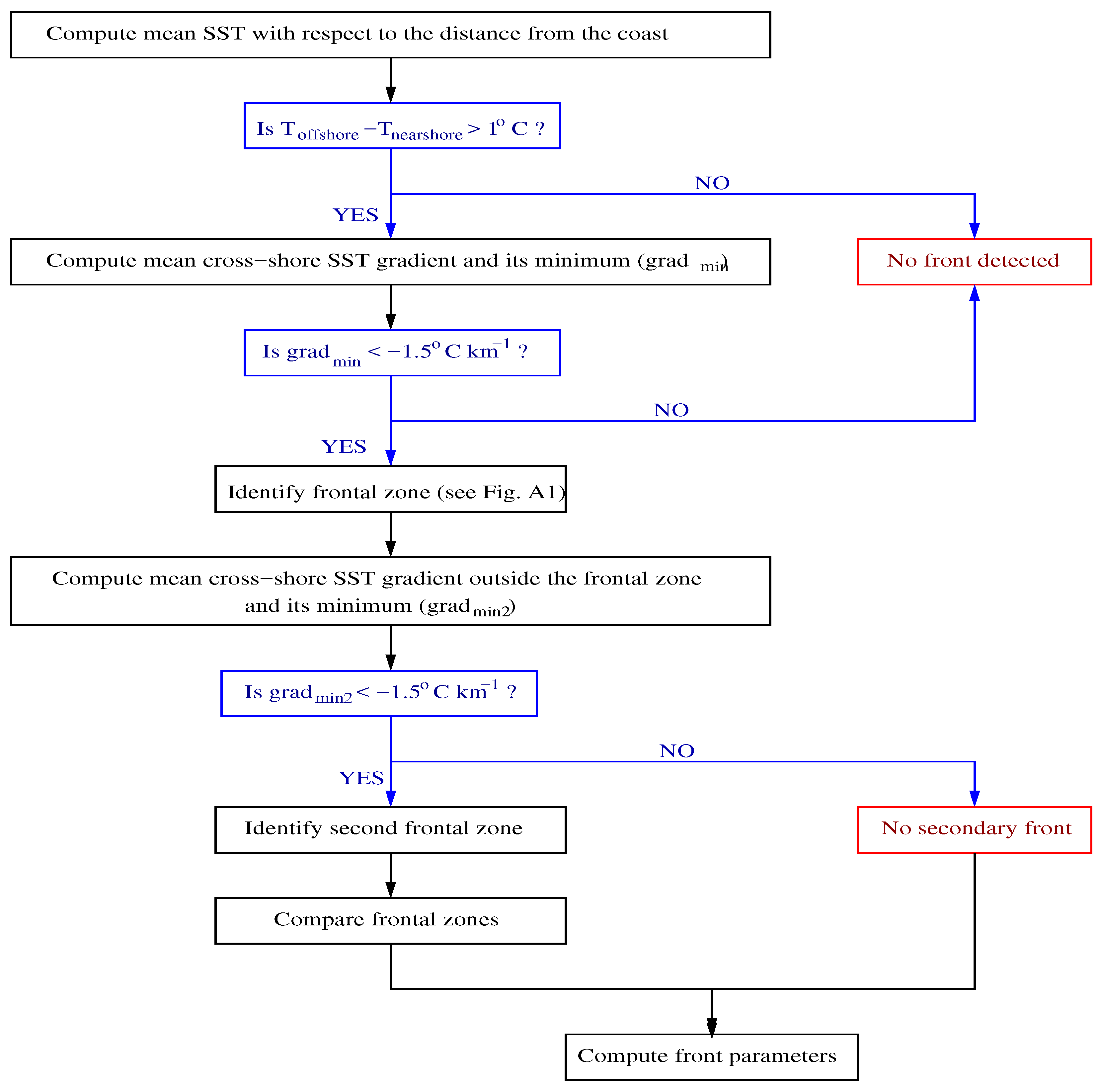
2.2.2. Front Detection
2.2.3. Determination of the Front Characteristics
2.3. Statistical Validation of the Detected Fronts
3. Results
3.1. Atmospheric and Oceanic Forcing
3.1.1. Local Atmospheric Forcing and Its Impact on the SST
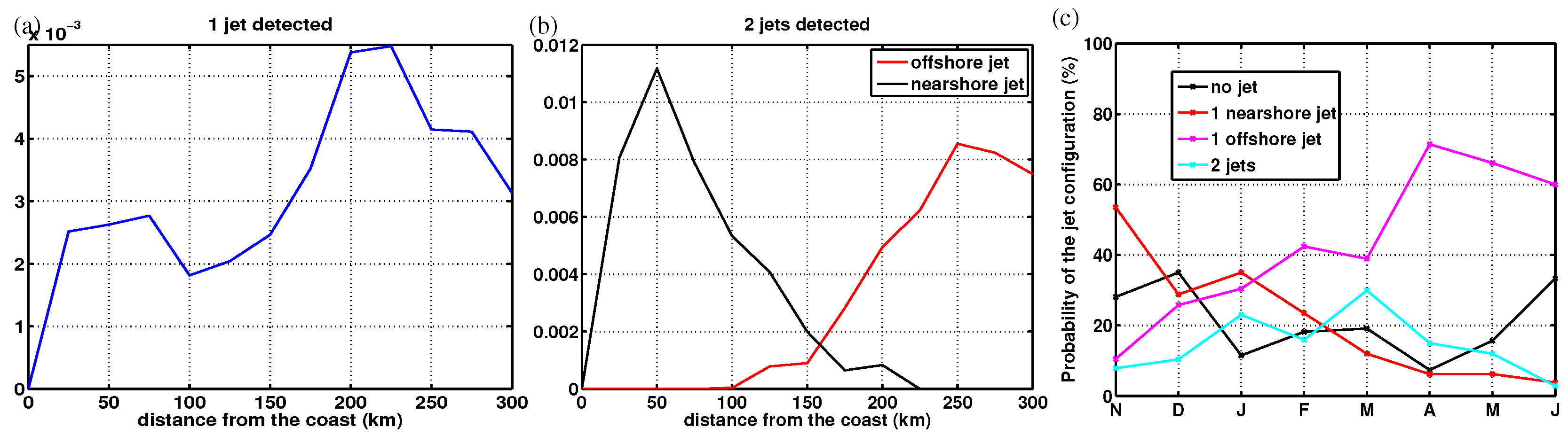
3.1.2. Coastal Jet Circulation
3.2. The Front Characteristics Variability
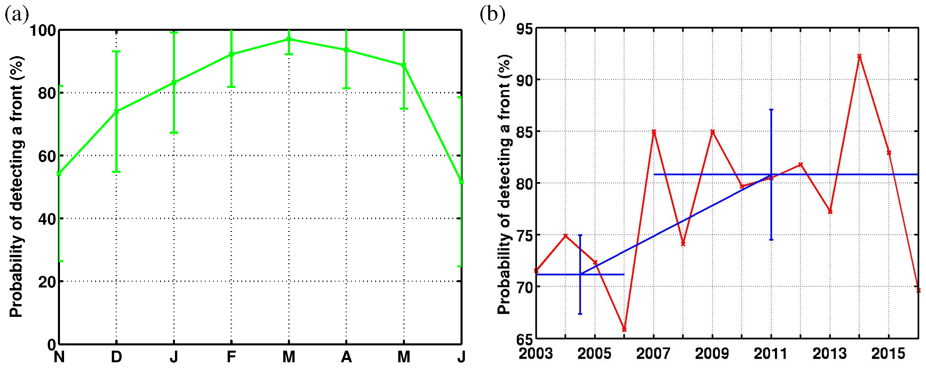
3.2.1. Probability of Detecting a Front
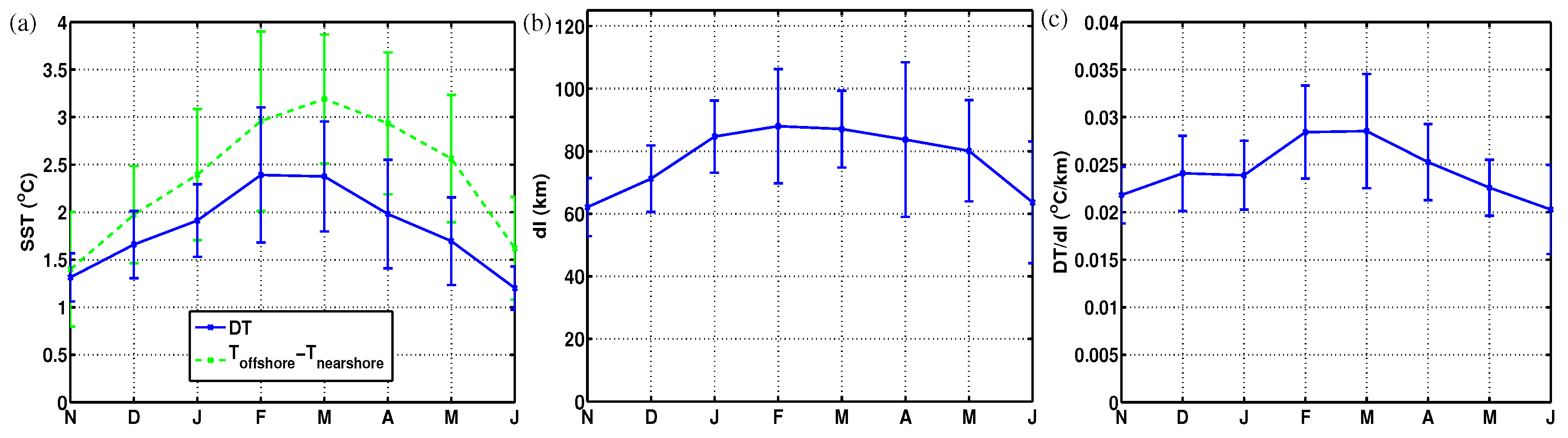
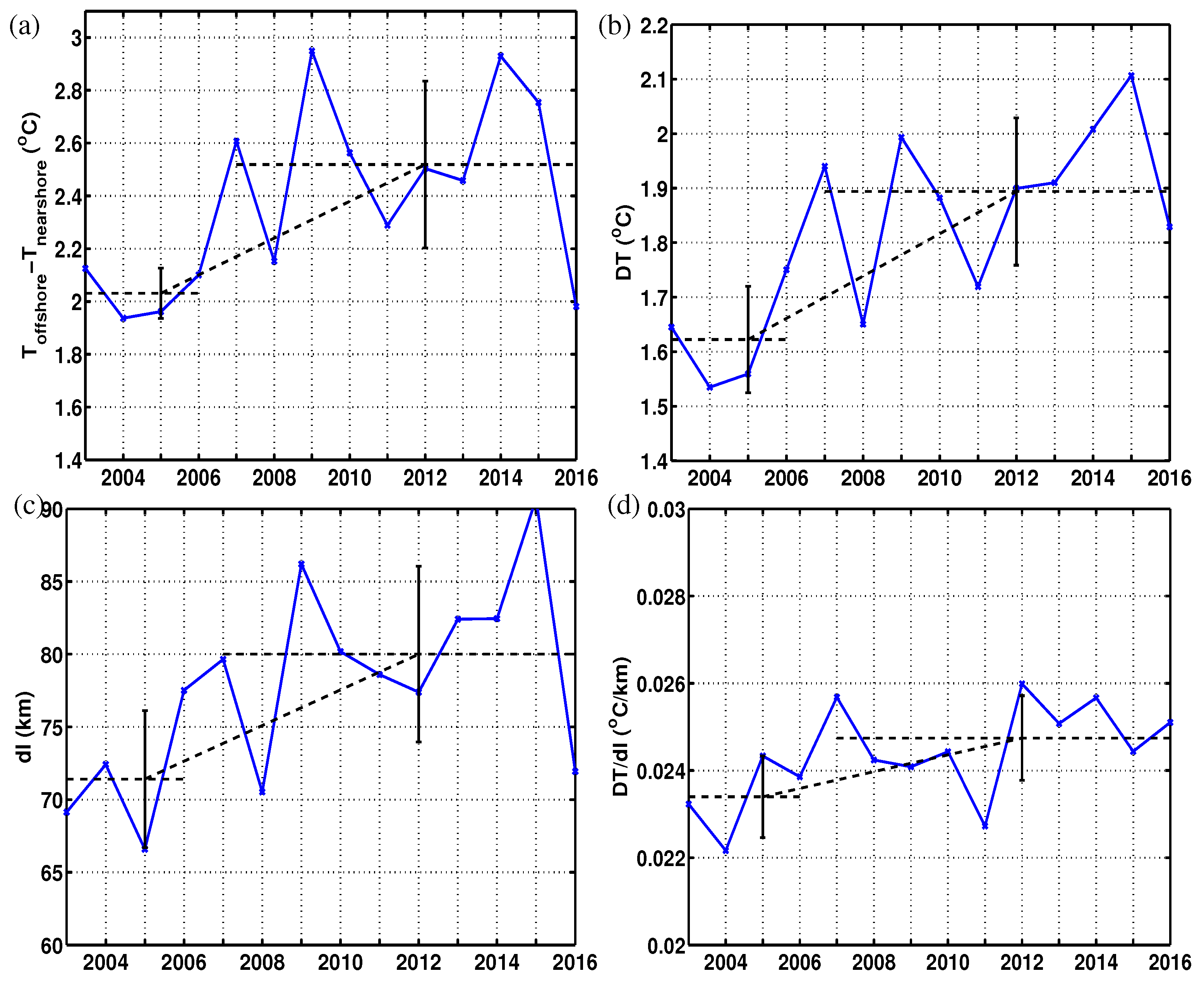
3.2.2. Front Intensity
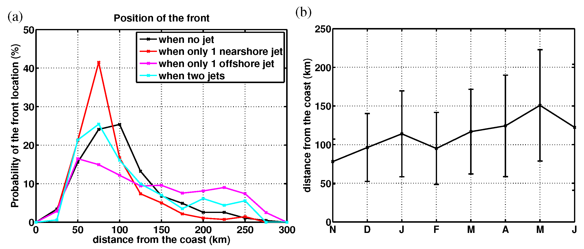
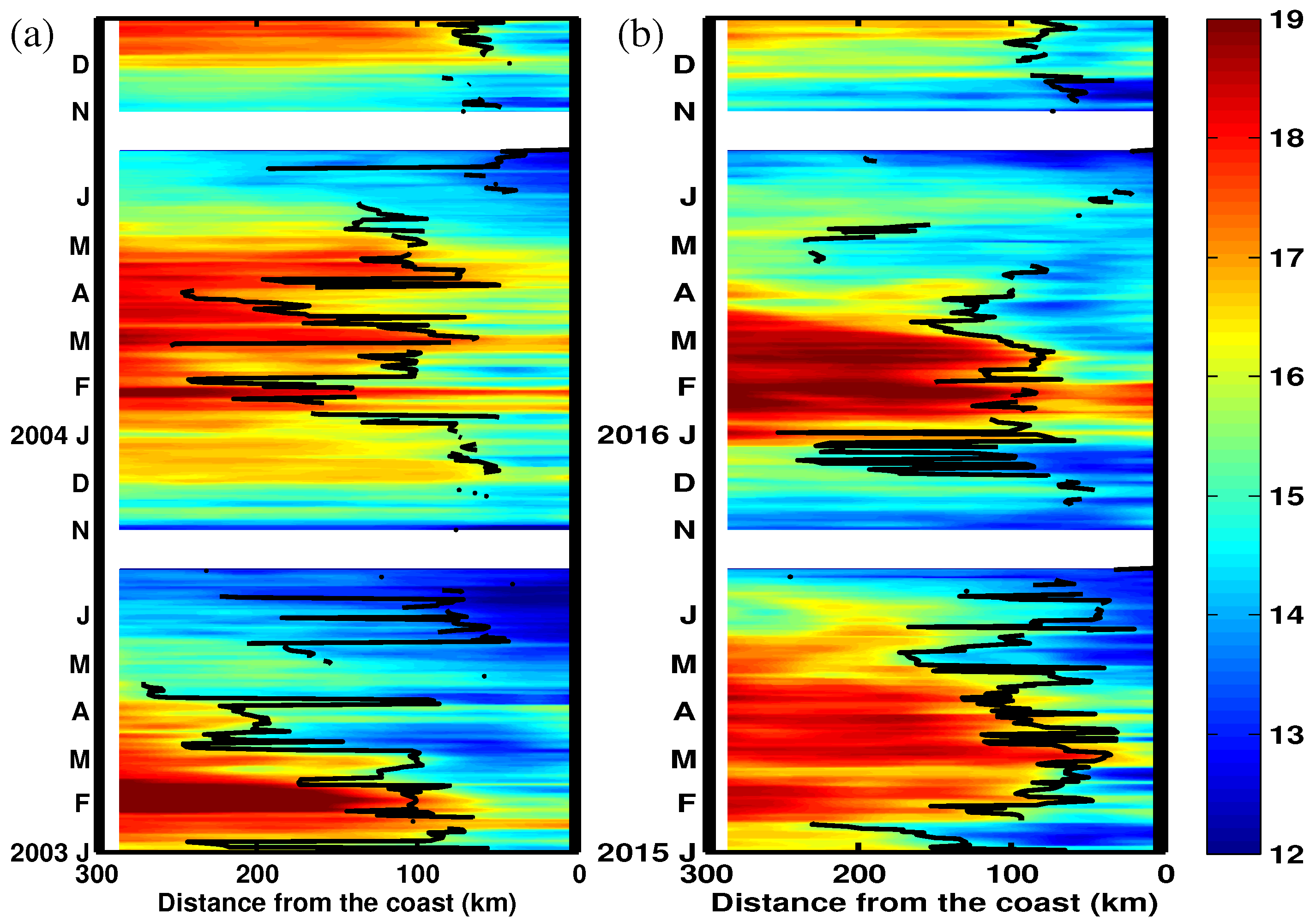
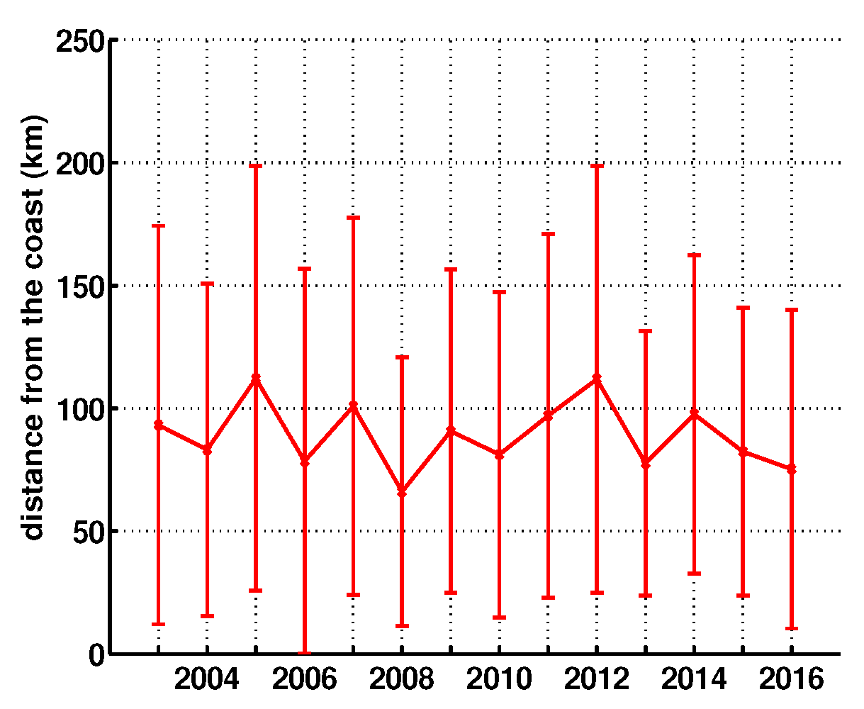
3.2.3. Front Position
4. Discussion
4.1. Strength and Limitations of the Front Detection Method
4.1.1. Strength
4.1.2. Limitations
4.2. Comparison of the Front Detection Method with Previous Works
4.2.1. Consistency with the Front Definition by Cayula and Cornillon (1992)
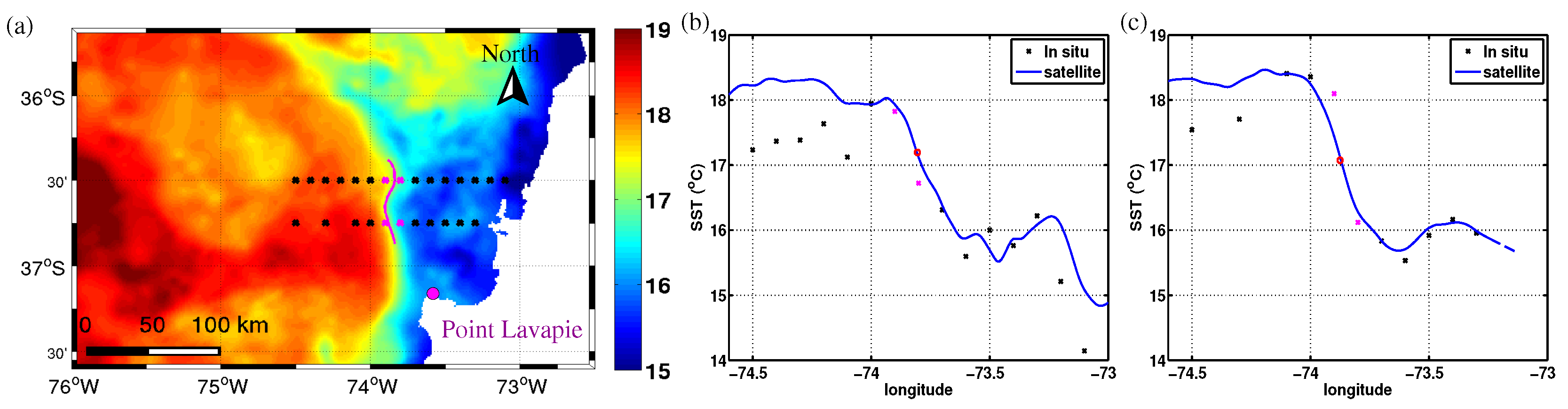
4.2.2. Consistency with In Situ Measurement
4.3. Front Characteristics Variability off Central Chile
4.3.1. Errors and Uncertainties
4.3.2. Jet Configuration and Front Position
4.3.3. Reinforcement of the Upwelling Front in EBUS
5. Conclusions
Author Contributions
Acknowledgments
Conflicts of Interest
Abbreviations
| EBUS | Eastern Boundary Upwelling System |
| CTZ | Coastal Transition Zone |
| SST | Sea Surface Temperature |
| HCS | Humboldt Current System |
| ENSO | El Niño Southern Oscillation |
| SSH | Sea Surface Height |
| Probability Density Function | |
| MUR | Multi-scale Ultra-high Resolution |
| NOCS | National Oceanography Center Southampton |
| ONI | Oceanic Niño Index |
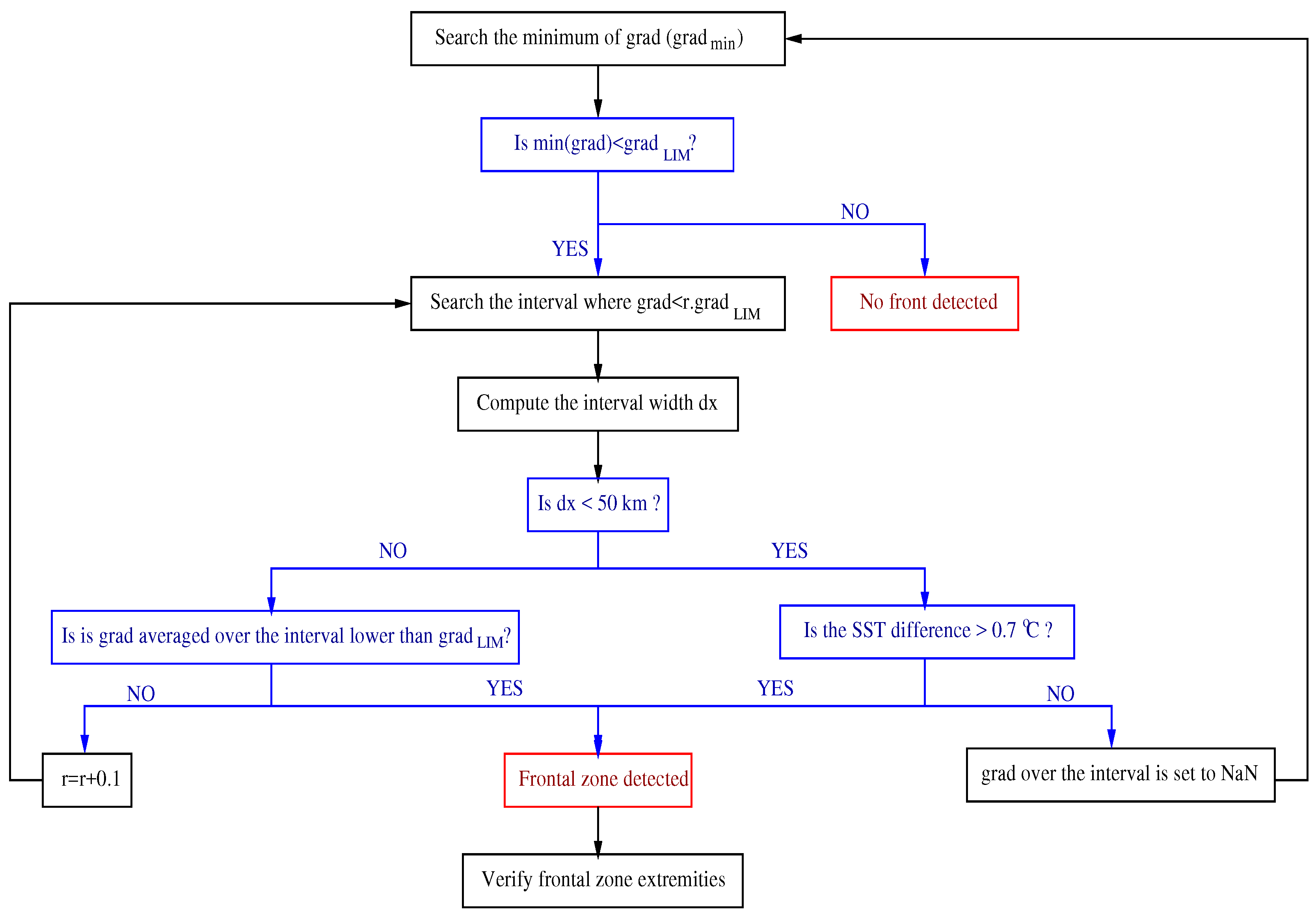
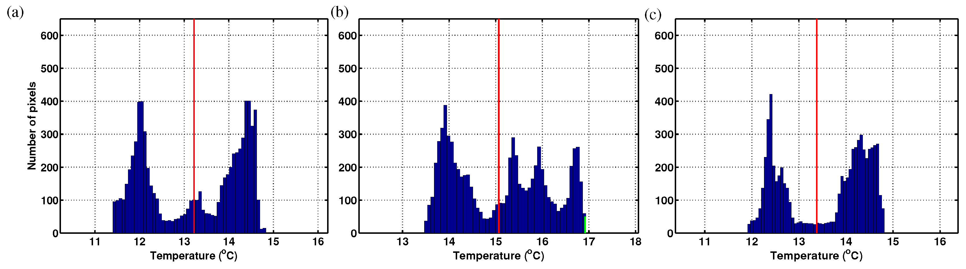
Appendix A. Strong Cross-Shore Gradient Zone “Frontal Zone”) Identification

References
- Lutjeharms, J.R.E.; Stockton, P.L. Kinematics of the upwelling front off southern Africa. S. Afr. J. Mar. Sci. 1987, 5, 35–49. [Google Scholar] [CrossRef]
- Austin, J.A.; Barth, J.A. Variation in the position of the upwelling front on the Oregon shelf. J. Geophys. Res. 2002, 107, 3180. [Google Scholar] [CrossRef]
- Peliz, A.; Rosa, T.L.; Santos, A.P.; Pissarra, J.L. Fronts, jets, and counter-flows in the Western Iberian upwelling system. J. Mar. Syst. 2002, 35, 61–77. [Google Scholar] [CrossRef]
- Durski, S.M.; Allen, J.S. Finite-amplitude evolution of instabilities associated with the coastal upwelling front. J. Phys. Oceanogr. 2005, 35, 1606–1628. [Google Scholar] [CrossRef]
- Strub, P.; James, C. Altimeter-derived variability of surface velocities in the California Current System: 2. Seasonal circulation and eddy statistics. Deep Sea Res. Part II Top. Stud. Oceanogr. 2000, 47, 831–870. [Google Scholar] [CrossRef]
- Morales, C.E.; Gonzalez, H.E.; Hormazabal, S.E.; Yuras, G.; Letelier, J.; Castro, L.R. The distribution of chlorophyll-a and dominant planktonic components in the coastal transition zone off Concepcion, central Chile, during different oceanographic conditions. Progr. Oceanogr. 2007, 75, 452–469. [Google Scholar] [CrossRef]
- Letelier, J.; Pizarro, O.; Nuñez, S. Seasonal variability of coastal upwelling and the upwelling front off central Chile. J. Geophys. Res. 2009, 114, C12009. [Google Scholar] [CrossRef]
- Brink, K. Upwelling fronts: Implications and unknowns. S. Afr. J. Mar. Sci. 1987, 5, 3–9. [Google Scholar] [CrossRef]
- Morales, C.E.; Hormazabal, S.E.; Correa-Ramirez, O.; Pizarro, O.; Silva, N.; Fernandez, C.; Anabalon, V.; Torreblanca, M. Mesoscale variability and nutrient-phytoplankton distributions off central-southern Chile during the upwelling season: The influence of mesoscale eddies. Progr. Oceanogr. 2012, 104, 17–29. [Google Scholar] [CrossRef]
- Menschel, E.; Gonzalez, H.E.; Giesecke, R. Coastal-oceanic distribution gradient of coccolithophores and their role in the carbonate flux of the upwelling system off Concepcion, Chile (36∘S). J. Plankton Res. 2016, 38, 798–817. [Google Scholar] [CrossRef]
- Tiedemann, M.; Brehmer, P. Larval fish assemblages across an upwelling front: Indication for active and passive retention. Estuar. Coast. Shelf Sci. 2017, 187, 118–133. [Google Scholar] [CrossRef]
- Demarcq, H.; Barlow, R.G.; Shillington, F.A. Climatology and variability of sea surface temperature and surface chlorophyll in the Benguela and Agulhas ecosystems as observed by satellite imagery. Afr. J. Mar. Sci. 2003, 25, 363–372. [Google Scholar] [CrossRef]
- Sobarzo, M.; Bravo, L.; Donoso, D.; Garcés-Vargas, J.; Schneider, W. Coastal upwelling and seasonal cycles that influence the water column over the continental shelf off central Chile. Progr. Oceanogr. 2007, 75, 363–382. [Google Scholar] [CrossRef]
- Morales, C.E.; Anabalon, V.; Bento, J.P.; Hormazabal, S.; Cornejo, M.; Correa-Ramirez, M.A.; Silva, N. Front-eddy influence on water column properties, phytoplankton community structure, and cross-shelf exchange of diatom taxa in the shelf-slope area off Concepcion (36–37∘S). J. Geophys. Res. Ocean. 2017, 122, 8944–8965. [Google Scholar] [CrossRef]
- Canny, J. A computational approach to edge detection. IEEE Trans. Pattern Anal. Mach. Intell. 1986, 8, 679–698. [Google Scholar] [CrossRef] [PubMed]
- Cayula, J.F.; Cornillon, P. Edge detection algorithm for SST images. J. Atmos. Ocean. Technol. 1992, 9, 67–80. [Google Scholar] [CrossRef]
- Pozo Vázquez, D.; Atae-Allah, C.; Luque Escamilla, P.L. Entropic approach to edge-detection for SST images. J. Atmos. Ocean. Technol. 1999, 16, 970–979. [Google Scholar] [CrossRef]
- Torres, J.A.; Guindos, F.; Peralta, M.; Cantón, M. Competitive neural-net-based system for the automatic detection of oceanic mesoscalar structures on AVHRR scenes. IEEE Trans. Geosci. Remote Sens. 2003, 41, 845–852. [Google Scholar] [CrossRef]
- Castelao, R.M.; Mavor, T.P.; Barth, J.A.; Breaker, L.C. Sea surface temperature fronts in the California Current System from geostationary satellite observations. J. Geophys. Res. 2006, 111, C09026. [Google Scholar] [CrossRef]
- Belkin, I.; O’Reilly, J. An algorithm for oceanic front detection in chlorophyll and SST satellite imagery. J. Mar. Syst. 2009, 78, 319–326. [Google Scholar] [CrossRef]
- Nieto, K.; Demarcq, H.; McClatchie, S. Mesoscale frontal structures in the Canary Upwelling System: New front and filament detection algorithms applied to spatial and temporal patters. Remote Sens. Environ. 2012, 123, 339–346. [Google Scholar] [CrossRef]
- Cayula, J.F.; Cornillon, P. Multi-image edge detection for SST images. J. Atmos. Ocean. Technol. 1995, 12, 821–829. [Google Scholar] [CrossRef]
- Diehl, S.F.; Budd, J.W.; Ullman, D.; Cayula, J.F. Geographic window sizes applied to remote sensing sea surface temperature front detection. J. Atmos. Ocean. Technol. 2002, 19, 1105–1113. [Google Scholar] [CrossRef]
- Hormazabal, S.; Shaffer, G.; Letelier, J.; Ulloa, O. Local and remote forcing of Sea Surface Temperature in the coastal upwelling system off Chile. J. Geophys. Res. Ocean. 2001, 106, 16657–16671. [Google Scholar] [CrossRef]
- Sobarzo, M.; Bravo, L.; Donoso, D.; Garces-Vargas, J.; Schneider, W. Coastal upwelling and seasonal cycles that influence the water column over the continental shelf off central Chile. Prog. Oceanogr. 2007, 75, 363–383. [Google Scholar] [CrossRef]
- Renault, L.; Dewitte, B.; Falvey, M.; Garreaud, R.; Echevin, V.; Bonjean, F. Impact of atmospheric coastal jet off central Chile on sea surface temperature from satellite observations (2000–2007). J. Geophys. Res. 2009, 114, C08006. [Google Scholar] [CrossRef]
- Aguirre, C.; Garreaud, R.D.; Rutllant, J.A. Surface ocean response to synoptic-scale variability in wind stress and heat fluxes off south-central Chile. Dyn. Atmos. Ocean. 2013, 65, 64–85. [Google Scholar] [CrossRef]
- Leth, O.; Middleton, J.F. A numerical study of the upwelling circulation off central Chile: Effects of remote oceanic forcing. J. Geophys. Res. 2006, 111, C12003. [Google Scholar] [CrossRef]
- Rutllant, J.A.; Masotti, I.; Calderón, J.; Vega, S.A. A comparison of spring coastal upwelling off central Chile at the extremes of the 1996–1997 ENSO cycle. Cont. Shelf Res. 2004, 24, 773–787. [Google Scholar] [CrossRef]
- Colas, F.; Capet, X.; McWilliams, J.; Shchepetkin, A. 1997–1998 El Niño off Peru: A numerical study. Prog. Oceanogr. 2008, 79, 138–155. [Google Scholar] [CrossRef]
- Aguirre, C.; Pizarro, O.; Strub, P.; Garreaud, R.; Barth, J. Seasonal dynamics of the near-surface alongshore flow off Central Chile. J. Geophys. Res. 2012, 117, C01006. [Google Scholar] [CrossRef]
- Leth, O.; Middleton, J.F. A mechanism for enhanced upwelling off central Chile: Eddy advection. J. Geophys. Res. 2004, 109, C1202. [Google Scholar] [CrossRef]
- Mesias, J.M.; Matano, R.P.; Strub, P.T. Dynamical analysis of the upwelling circulation off central Chile. J. Geophys. Res. 2003, 108, 3085. [Google Scholar] [CrossRef]
- Wang, Y.; Castelao, R.M.; Yuan, Y. Seasonal variability of alongshore winds and sea surface temperature fronts in Eastern Boundary Current Systems. J. Geophys. Res. Ocean. 2015, 120, 2385–2400. [Google Scholar] [CrossRef]
- SERNAPESCA. Anuario Estadístico de Pesca 2006; Ministerio de Economia, Fomento y Turismo: Santiago, Chile, 2006. [Google Scholar]
- Physical Oceanography Distributed Active Archive Center. JPL MUR MEaSUREs Project. 2015. GHRSST Level 4 MUR Global Foundation Sea Surface Temperature Analysis (v4.1). Version 4.1.; Physical Oceanography Distributed Active Archive Center: Pasadena, CA, USA, 2015. [Google Scholar] [CrossRef]
- Pujol, M.I.; Faugère, Y.; Taburet, G.; Dupuy, S.; Pelloquin, C.; Ablain, M.; Picot, N. DUACS DT2014: The new multi-mission altimeter data set reprocessed over 20 years. Ocean Sci. 2016, 12, 1067–1090. [Google Scholar] [CrossRef]
- Bentamy, A.; Grodsky, S.; Carton, J.; Croizé-Fillon, D.; Chapron, B. Matching ASCAT and QuikSCAT winds. J. Geophys. Res. 2012, 117, C02011. [Google Scholar] [CrossRef]
- Desbiolles, F.; Bentamy, A.; Blanke, B.; Roy, C.; Mestas-Nunez, A.; Grodsky, S.; Herbette, S.; Cambon, G.; Maes, C. Two decades [1992–2012] of surface wind analyses based on satellite scatterometer observations. J. Mar. Syst. 2017, 168, 38–56. [Google Scholar] [CrossRef]
- National Oceanography Centre, Southampton, UK. NOCS Surface Flux Dataset v2.0. 2008. Available online: http://rda.ucar.edu/datasets/ds260.3/ (accessed on 24 January 2018).
- Berry, D.I.; Kent, E.C. Air-sea fluxes from ICOADS: The construction of a new gridded dataset with uncertainty estimates. Int. J. Climatol. 2011, 31, 987–1001. [Google Scholar] [CrossRef]
- NOAA. Cold and Warm Episodes by Season. 2018. Available online: http://origin.cpc.ncep.noaa.gov/products/analysis_monitoring/ensostuff/ONI_v5.php (accessed on 08 April 2018).
- Schneider, W.; Donoso, D.; Garcés-Vargas, J.; Escribano, R. Water-column cooling and sea surface salinity increase in the upwelling region off Central-South Chile driven by a poleward displacement of the South Pacific High. Prog. Oceanogr. 2017, 151, 38–48. [Google Scholar] [CrossRef]
- Morales, C.E.; Hormazabal, S.; Andrade, I.; Correa-Ramirez, M.A. Time-space variability of chlorophyll-a and associated physical variables within the region off central-southern Chile. Remote Sens. 2013, 5, 5550–5571. [Google Scholar] [CrossRef]
- Castelao, R.M.; Barth, J.A. The role of wind stress curl in jet separation at a cape. J. Phys. Oceanogr. 2007, 37, 2652–2671. [Google Scholar] [CrossRef]
- Kelly, K.A.; Caruso, M.J.; Austin, J.A. Wind-forced variations in sea surface height in the northeast Pacific ocean. J. Phys. Oceanogr. 1993, 23, 2392–2411. [Google Scholar] [CrossRef]
- Lorenzo, E.D. Seasonal dynamics of the surface circulation in the Southern California Current System. Deep Sea Res. Part II Top. Stud. Oceanogr. 2003, 50, 2371–2388. [Google Scholar] [CrossRef]
- Barth, J.A.; Pierce, S.D.; Cowles, T.J. Mesoscale structure and its seasonal evolution in the northern California Current System. Deep Sea Res. Part II Top. Stud. Oceanogr. 2005, 52, 5–28. [Google Scholar] [CrossRef]
- Lynn, R.J.; Bograd, S.J.; Chereskin, T.K.; Huyer, A. Seasonal renewal of the California Current: The spring transition off California. J. Geophys. Res. Ocean. 2003, 108, 3279. [Google Scholar] [CrossRef]
- Belmadani, A.; Echevin, V.; Codron, F.; Takahashi, K.; Junquas, C. What dynamics drive future winds scenarios off Peru and Chile? Clim. Dyn. 2014, 43, 1893–1914. [Google Scholar] [CrossRef]
- Bakun, A.; Weeks, S.J. The marine ecosystem off Peru: What are the secrets of its fishery productivity and what might its future hold? Prog. Oceanogr. 2008, 79, 290–299. [Google Scholar] [CrossRef]
- Goubanova, K.; Echevin, V.; Dewitte, B.; Codron, F.; Takahashi, K.; Terray, P.; Vrac, M. Statistical downscaling of sea-surface wind over the Peru–Chile upwelling region: Diagnosing the impact of climate change from the IPSL-CM4 model. Clim. Dyn. 2011, 36, 1365–1378. [Google Scholar] [CrossRef]
- Sydeman, W.; García-Reyes, M.; Schoeman, D.S.; Rykaczewski, R.R.; Thompson, S.A.; Black, B.A.; Bograd, S.J. Climate change and wind intensification in coastal upwelling ecosystems. Science 2014, 345, 77–80. [Google Scholar] [CrossRef] [PubMed]
- Marchesiello, P.; McWilliams, J.C.; Shchepetkin, A. Equilibrium structure and dynamics of the California current system. J. Phys. Oceanogr. 2003, 33, 753–783. [Google Scholar] [CrossRef]
- Belmadani, A.; Echevin, V.; Dewitte, B.; Colas, F. Equatorially forced intraseasonal propagations along the Peru-Chile coast and their relation with the nearshore eddy activity in 1992–2000: A modeling study. J. Geophys. Res. 2012, 117, C04025. [Google Scholar] [CrossRef]
- Pelegrí, J.; Arístegui, J.; Cana, L.; González-Dávila, M.; Hernández-Guerra, A.; Hernández-León, S.; Marrero-Díaz, A.; Montero, M.; Sangrà, P.; Santana-Casiano, M. Coupling between the open ocean and the coastal upwelling region off northwest Africa: Water recirculation and offshore pumping of organic matter. J. Mar. Syst. 2005, 54, 3–37. [Google Scholar] [CrossRef]
- Capet, X.; McWilliams, J.C.; Molemaker, M.J.; Shchepetkin, A.F. Mesoscale to submesoscale transition in the California Current System. Part II: Frontal processes. J. Phys. Oceanogr. 2008, 38, 44–64. [Google Scholar] [CrossRef]
- Hösen, E.; Möller, J.; Jochumsen, K.; Quadfasel, D. Scales and properties of cold filaments in the Benguela upwelling system off Lüderitz. J. Geophys. Res. Ocean. 2016, 121, 1896–1913. [Google Scholar] [CrossRef]
- Colas, F.; McWilliams, J.C.; Capet, X.; Kurian, J. Heat balance and eddies in the Peru-Chile current system. Clim. Dyn. 2012, 39, 509–529. [Google Scholar] [CrossRef]
- Castelao, R.M.; Wang, Y. Wind-driven variability in sea surface temperature front distribution in the California Current System. J. Geophys. Res. Ocean. 2014, 119, 1861–1875. [Google Scholar] [CrossRef]
- Vazquez-Cuervo, J.; Torres, H.S.; Menemenlis, D.; Chin, T.; Armstrong, E.M. Relationship between SST gradients and upwelling off Peru and Chile: Model/satellite data analysis. Int. J. Remote Sens. 2017, 38, 6599–6622. [Google Scholar] [CrossRef]
- Kahru, M.; Di Lorenzo, E.; Manzano-Sarabia, M.; Mitchell, B. Spatial and temporal statistics of Sea Surface Temperature and chlorophyll fronts in the California Current. J. Plankton Res. 2012, 34, 749–760. [Google Scholar] [CrossRef]
- Capet, X.; McWilliams, J.C.; Molemaker, M.J.; Shchepetkin, A.F. Mesoscale to submesoscale transition in the California Current System. Part I: Flow structure, eddy flux, and observational tests. J. Phys. Oceanogr. 2008, 38, 29–43. [Google Scholar] [CrossRef]
- Mahadevan, A. The impact of submesoscale physics on primary productivity of plankton. Ann. Rev. Mar. Sci. 2016, 8, 161–184. [Google Scholar] [CrossRef] [PubMed]
- McWilliams, J.C. Submesoscale currents in the ocean. Proc. R. Soc. A 2016, 472, 20160117. [Google Scholar] [CrossRef] [PubMed]
- D’Asaro, E.; Lee, C.; Rainville, L.; Harcourt, R.; Thomas, L. Enhanced turbulence and energy dissipation at ocean fronts. Science 2011, 15, 318–322. [Google Scholar] [CrossRef] [PubMed]
- Johnston, T.; Rudnick, D.L.; Pallas-Sanz, E. Elevated mixing at a front. J. Geophys. Res. 2011, 116, C11033. [Google Scholar] [CrossRef]
- Merlivat, L.; Davila, M.G.; Caniaux, G.; Boutin, J.; Reverdin, G. Mesoscale and diel to monthly variability of CO2 and carbon fluxes at the ocean surface in the northeastern Atlantic. J. Geophys. Res. 2009, 114, C03010. [Google Scholar] [CrossRef]
- Ferrari, R. A frontal challenge for climate models. Science 2011, 332, 316–317. [Google Scholar] [CrossRef] [PubMed]
- Köhn, E.E.; Thomsen, S.; Arévalo-Martínez, D.L.; Kanzow, T. Submesoscale CO2 variability across an upwelling front off Peru. Ocean Sci. 2017, 13, 1017–1033. [Google Scholar] [CrossRef]
- Lévy, M.; Franks, P.; Martin, A.P.; Rivière, P. Bringing physics to life at the submesoscale. J. Geophys. Res. 2012, 39, L14602. [Google Scholar] [CrossRef]
- Stukel, M.R.; Aluwihare, L.I.; Barbeau, K.A.; Chekalyuk, A.M.; Goericke, R.; Miller, A.J.; Ohman, M.D.; Ruacho, A.; Song, H.; Stephens, B.M.; et al. Mesoscale ocean fronts enhance carbon export due to gravitational sinking and subduction. PNAS 2017, 114, 1252–1257. [Google Scholar] [CrossRef] [PubMed]
- Thomsen, S.; Kanzow, T.; Colas, F.; Echevin, V.; Krahmann, G.; Engel, A. Do submesoscale frontal processes ventilate the oxygen minimum zone off Peru? Geophys. Res. Lett. 2016, 43, 8133–8142. [Google Scholar] [CrossRef]
- Li, Q.P.; Franks, P.J.S.; Ohman, M.; Landry, M.R. Enhanced nitrate fluxes and biological processes at a frontal zone in the Southern California Current System. J. Plankton Res. 2012, 34, 790–801. [Google Scholar] [CrossRef]
- Taylor, A.G.; Goericke, R.; Landry, M.R.; Selph, K.E.; Wick, D.A.; Roadman, M.J. Sharp gradients in phytoplankton community structure across a frontal zone in the California Current Ecosystem. J. Plankton Res. 2012, 34, 778–789. [Google Scholar] [CrossRef]
- Ohman, M.D.; Powell, J.R.; Picheral, M.; Jensen, D. Mesozooplankton and particulate matter responses to a deep-water frontal system in the southern California Current System. J. Plankton Res. 2012, 34, 815–827. [Google Scholar] [CrossRef]
- Krause, J.W.; Brzezinski, M.A.; Goericke, R.; Landry, M.R.; Ohman, M.D.; Stukel, M.R.; Taylor, A.G. Variability in diatom contributions to biomass, organic matter production and export across a frontal gradient in the California Current Ecosystem. J. Geophys. Res. Ocean. 2015, 120, 1032–1047. [Google Scholar] [CrossRef]
- Böttjer, D.; Morales, C.E. Nanoplanktonic assemblages in the upwelling area off Concepción (∼36∘S), central Chile: Abundance, biomass, and grazing potential during the annual cycle. Progr. Oceanogr. 2007, 75, 415–434. [Google Scholar] [CrossRef]
- Castro, L.R.; Troncoso, V.A.; Figueroa, D.R. Fine-scale vertical distribution of coastal and offshore copepods in the Golfo de Arauco, central Chile, during the upwelling season. Prog. Oceanogr. 2007, 75, 486–500. [Google Scholar] [CrossRef]


| 10 January 2004 | 0.9 | 5.1 |
| 19 May 2004 | 0.8 | 4.4 |
| 02 March 2005 | 0.9 | 5.1 |
| 10 March 2005 | 0.9 | 5.1 |
| 05 April 2005 | 0.8 | 4.6 |
| 11 January 2005 | 0.8 | 4.8 |
| 15 January 2007 | 0.7 | 3.5 |
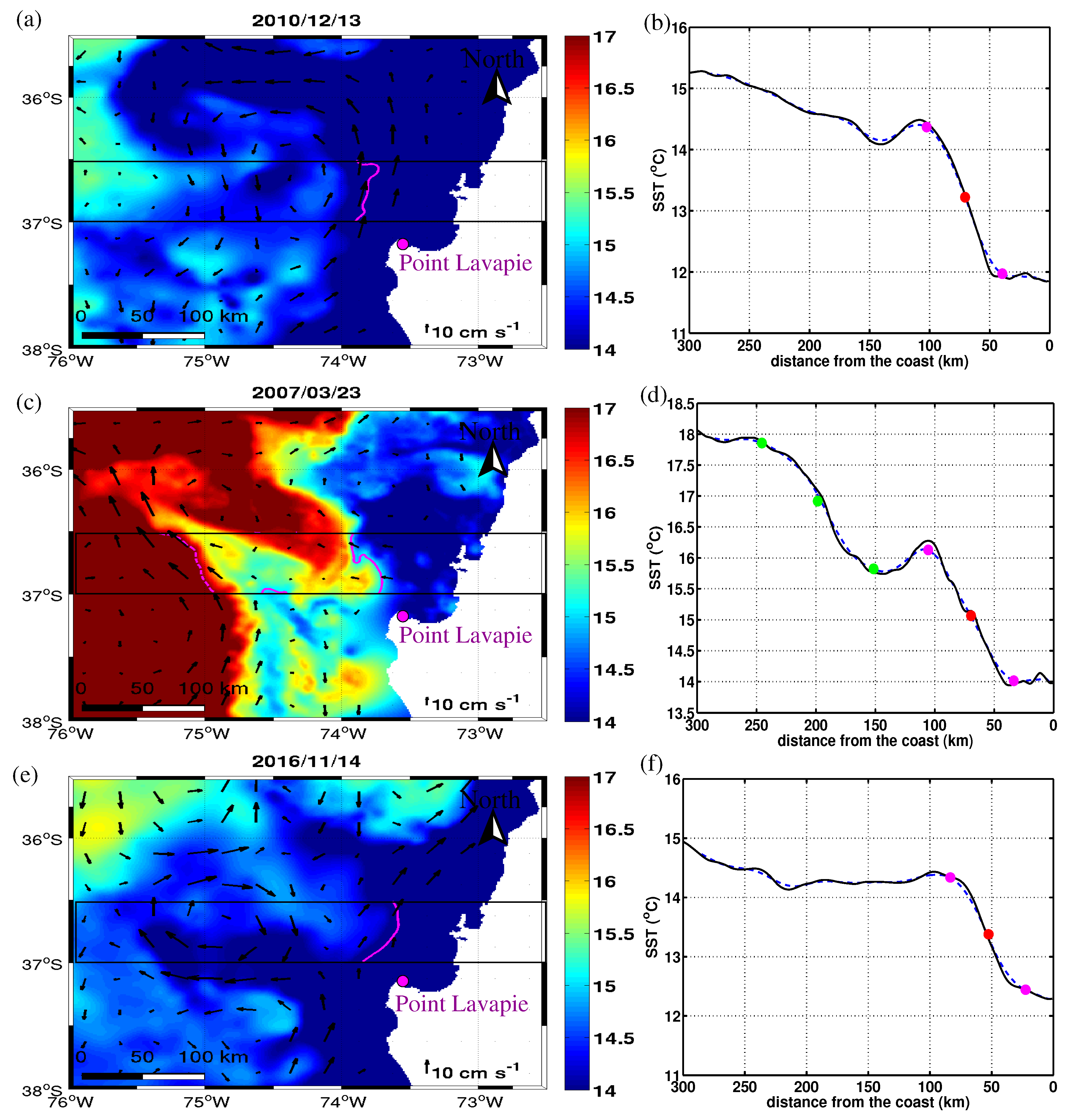
| 23 March 2007 | 0.8 | 4.0 |
| 10 March 2009 | 0.9 | 5.8 |
| 13 December 2010 | 0.9 | 5.0 |
| 14 November 2016 | 0.9 | 6.1 |
| R(,) | R(,) | R(,) | |
|---|---|---|---|
| monthly mean | 0.86 | 0.78 | 0.77 |
| yearly mean | 0.88 | 0.89 | 0.64 |
| climatological seasonal cycle | 0.93 | 0.93 | 0.97 |
© 2018 by the authors. Licensee MDPI, Basel, Switzerland. This article is an open access article distributed under the terms and conditions of the Creative Commons Attribution (CC BY) license (http://creativecommons.org/licenses/by/4.0/).
Share and Cite
Oerder, V.; Bento, J.P.; Morales, C.E.; Hormazabal, S.; Pizarro, O. Coastal Upwelling Front Detection off Central Chile (36.5–37°S) and Spatio-Temporal Variability of Frontal Characteristics. Remote Sens. 2018, 10, 690. https://doi.org/10.3390/rs10050690
Oerder V, Bento JP, Morales CE, Hormazabal S, Pizarro O. Coastal Upwelling Front Detection off Central Chile (36.5–37°S) and Spatio-Temporal Variability of Frontal Characteristics. Remote Sensing. 2018; 10(5):690. https://doi.org/10.3390/rs10050690
Chicago/Turabian StyleOerder, Vera, Joaquim P. Bento, Carmen E. Morales, Samuel Hormazabal, and Oscar Pizarro. 2018. "Coastal Upwelling Front Detection off Central Chile (36.5–37°S) and Spatio-Temporal Variability of Frontal Characteristics" Remote Sensing 10, no. 5: 690. https://doi.org/10.3390/rs10050690
APA StyleOerder, V., Bento, J. P., Morales, C. E., Hormazabal, S., & Pizarro, O. (2018). Coastal Upwelling Front Detection off Central Chile (36.5–37°S) and Spatio-Temporal Variability of Frontal Characteristics. Remote Sensing, 10(5), 690. https://doi.org/10.3390/rs10050690