Article

Registration for Optical Multimodal Remote Sensing Images Based on FAST Detection, Window Selection, and Histogram Specification

1
College of Resource and Environment, Huazhong Agricultural University, 1 Shizishan Street, Wuhan 430070, China
2
Key Laboratory of Arable Land Conservation (Middle and Lower Reaches of Yangtse River), Ministry of Agriculture, 1 Shizishan Street, Wuhan 430070, China
3
USDA-Agricultural Research Service, Aerial Application Technology Research Unit, 3103 F & B Road, College Station, TX 77845, USA
4
College of Mechanical and Electronic Engineering, Northwest A&F University, 22 Xinong Road, Yangling 712100, China
5
Department of Biological Systems Engineering, University of Nebraska-Lincoln, 3605 Fair Street, Lincoln, NE 68583, USA
6
Texas A&M AgriLife Research and Extension Center, Beaumont, TX 77713, USA
7
Anhui Engineering Laboratory of Agro-Ecological Big Data, Anhui University, Hefei 230601, China
8
College of Engineering, Huazhong Agricultural University, 1 Shizishan Street, Wuhan 430070, China
*
Author to whom correspondence should be addressed.
Remote Sens. 2018, 10(5), 663; https://doi.org/10.3390/rs10050663
Submission received: 23 March 2018 / Revised: 16 April 2018 / Accepted: 21 April 2018 / Published: 24 April 2018
(This article belongs to the Section Remote Sensing Image Processing)

Abstract

:
In recent years, digital frame cameras have been increasingly used for remote sensing applications. However, it is always a challenge to align or register images captured with different cameras or different imaging sensor units. In this research, a novel registration method was proposed. Coarse registration was first applied to approximately align the sensed and reference images. Window selection was then used to reduce the search space and a histogram specification was applied to optimize the grayscale similarity between the images. After comparisons with other commonly-used detectors, the fast corner detector, FAST (Features from Accelerated Segment Test), was selected to extract the feature points. The matching point pairs were then detected between the images, the outliers were eliminated, and geometric transformation was performed. The appropriate window size was searched and set to one-tenth of the image width. The images that were acquired by a two-camera system, a camera with five imaging sensors, and a camera with replaceable filters mounted on a manned aircraft, an unmanned aerial vehicle, and a ground-based platform, respectively, were used to evaluate the performance of the proposed method. The image analysis results showed that, through the appropriate window selection and histogram specification, the number of correctly matched point pairs had increased by 11.30 times, and that the correct matching rate had increased by 36%, compared with the results based on FAST alone. The root mean square error (RMSE) in the x and y directions was generally within 0.5 pixels. In comparison with the binary robust invariant scalable keypoints (BRISK), curvature scale space (CSS), Harris, speed up robust features (SURF), and commercial software ERDAS and ENVI, this method resulted in larger numbers of correct matching pairs and smaller, more consistent RMSE. Furthermore, it was not necessary to choose any tie control points manually before registration. The results from this study indicate that the proposed method can be effective for registering optical multimodal remote sensing images that have been captured with different imaging sensors.

Graphical Abstract

1. Introduction

Image registration is an important image pre-processing procedure [1] that is required to align the images that are captured with different imaging sensors in remote sensing. Depending on particular applications, image registration involves the alignment of two or more images from optical imaging cameras or image data from other sources, such as digital elevation models [2], captured at different times and from different viewpoints [3] or by different sensors [4]. Through image registration, temporal images could be used for a time series analysis [5], and images from different viewpoints could generate new data, such as digital surface models (DSM) [6]. Although some remote sensing sensors can capture multispectral images without the need for image alignment, most airborne multispectral imaging systems capture multispectral images with multiple cameras or imaging sensors that require image-to-image alignment.
With the development of small unmanned aerial vehicles (UAVs) as well as the miniaturization of digital cameras in recent years, digital frame cameras are commonly used to capture aerial images for remote sensing applications [7]. Most digital frame cameras can only obtain red, green, and blue (RGB) color images. However, in many applications, such as in agriculture and natural resources, which focus on vegetation, cameras with visible bands alone cannot meet the requirement for vegetation monitoring. Therefore, modified consumer-grade cameras have increasingly been used to capture near-infrared (NIR) band images. Some imaging systems employ two or three separate consumer-grade cameras with one original camera to capture RGB spectral bands and the other one or two cameras are modified to capture red-edge (RDG) and/or NIR band images [8]. Some imaging systems integrate four or more imaging sensor units with one sensor for each spectral band. This type of imaging system usually has a common trigger to simultaneously capture and store images from the separate imaging units [9,10]. In laboratory or field experiments, a single camera is sometimes used to capture multispectral band images by changing different filters [11]. Some commonly-used multispectral imaging systems that are based on digital frame cameras are shown in Figure 1.
Although imaging systems that are based on digital frame cameras require image registration and radiometric calibration, they have many advantages for remote sensing, including their low cost, small size, and ease of use [12]. Unlike some scientific multispectral or hyperspectral cameras, which are based on the line array sensors, which do not need alignment, commonly-used multispectral cameras with frame sensors require all of the spectral bands to be aligned to one another. As all of the bands have different spectral ranges, it is sometimes difficult to identify common feature points among the band images, especially between the visible and NIR bands.
The automatic image registration methods are usually characterized as area-based or feature-based [14]. Area-based methods are mainly based on cross-correlation, Fourier techniques, mutual information, and optimization algorithms [15]. Area-based algorithms are usually exploited for directly matching image intensities, instead of constructing an explicit correspondence by local shapes or structures in the two images [14,16], which are limited by the matching window size and similarity of the image pairs. In addition, intensities that are extracted by area-based methods contain little explicit information, which causes unreliable registration results [17]. Therefore, area-based methods are inadequate for multimodal remote sensing images registration, since a huge discrepancy exists between the images that are to be matched, because of the differences in the spectral response ranges of the sensors.
Therefore, for multi-sensor image registration, feature-based techniques are commonly used, because these algorithms usually extract salient features, such as points, contours, and regions [18]. Feature-based registration algorithms extract distinctive, highly informative feature objects first. Some operators, such as scale-invariant feature transform (SIFT) [19,20,21], curvature scale space (CSS), Harris [22], speed up robust features (SURF) [23], and features from accelerated segment test (FAST) [24] are frequently used for feature point extraction. Many studies have compared the performances of various point detectors, proving that only a few are useful for the registration of remote sensing images, as a result of their characteristic of being computationally intensive [25].
The overall goal of this study was to develop a novel method for the registration of optical multimodal remote sensing images that were acquired by digital frame cameras, in order to increase matching points and matching accuracy, as compared to the commonly-used methods. The specific objectives were as follows: (1) select a feasible detector for the feature extraction from multimodal remote sensing images, by comparing the detection speed and correct matching rate; (2) optimize the window size in order to limit the scope of the image registration and to increase the correct matching pair numbers and correct matching rate; and (3) use histogram specification to improve the grayscale similarity between the subimages within windows.
The rest of this paper is organized as follows. In Section 2, imaging systems, test images, and test platforms are introduced and the proposed registration method is described in detail. The registration results are presented and analyzed in Section 3. In Section 4, the appropriate window size selection and the importance of histogram specification within windows are discussed, and the proposed method is compared with the state-of-the-art methods and commercial software, ERDAS and ENVI. Finally, conclusions are drawn in Section 5.

2. Materials and Methods

2.1. Imaging Systems and Test Images

In this study, three typical multispectral imaging systems were used, including a single camera with changeable filters, a dual-camera imaging system, and a five-band multi-lens camera. Images that were captured by the three imaging systems were used for image registration.

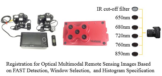
2.1.1. Multispectral Imaging Camera Based on Changeable Filters

A Nikon D7000 camera with a Nikon 50 mm f/1.4D fixed focus lens (Nikon, Inc., Tokyo, Japan) was modified as a multispectral imaging unit (Figure 1). The camera was used to capture RGB images and different NIR images of rice plants, by replacing the NIR-blocking filter in front of the sensor with different filters (IR-cut filters and 650 nm, 680 nm, 720 nm, 760 nm, and 850 nm long-pass NIR filters). Each image was recorded in 8-bit tagged image file format (TIFF) with 4928 × 3264 pixels, and was named Image Set I (Figure 2). This unit was the ground-based imaging platform that was typically used in laboratory settings, with the same optical axis and angular field of view.

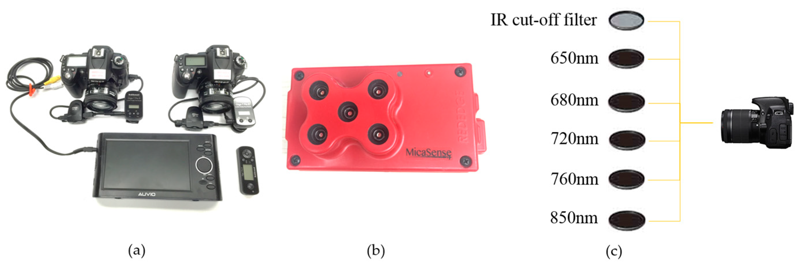
2.1.2. Dual-Camera Imaging System

A multispectral imaging system with two consumer-grade cameras, that was assembled by the scientists at the Aerial Application Technology Research Unit at the U.S. Department of Agriculture-Agricultural Research Service’s Southern Plains Agricultural Research Center in College Station, Texas, was used [8]. This imaging system included two Nikon D90 digital complementary metal–oxide–semiconductor (CMOS) cameras with Nikon AF Nikkor 24 mm f/2.8D lenses (Nikon, Inc., Melville, NY, USA). One camera was used to capture the three-band RGB images. The other camera was modified to capture NIR images, after the infrared-blocking filter installed in front of the CMOS of the camera was replaced with a 720 nm long-pass filter (Life Pixel Infrared, Mukilteo, WA, USA). This dual-camera imaging system was attached via a camera mount box on to an Air Tractor AT-402B agricultural aircraft. The images were taken under sunny conditions from a cropping area near College Station, Texas, USA with a ground speed of 225 km/h (140 mph), at an altitude of approximate 1524 m (5000 ft.) above the ground level, on 15 July 2015. Each image contained 4288 × 2848 pixels and was recorded in both joint photographic experts group (JPEG) and 12-bit raw format. Figure 3 shows a pair of RGB and NIR images, referred to as Global Image Set II. A subset pair of the two images, referred to as Local Set II, is also shown in Figure 3. It can be seen from the RGB and NIR images, that the contrast of the NIR image was far less than that of the RGB visible image.

2.1.3. Five-Band Multispectral Imaging System
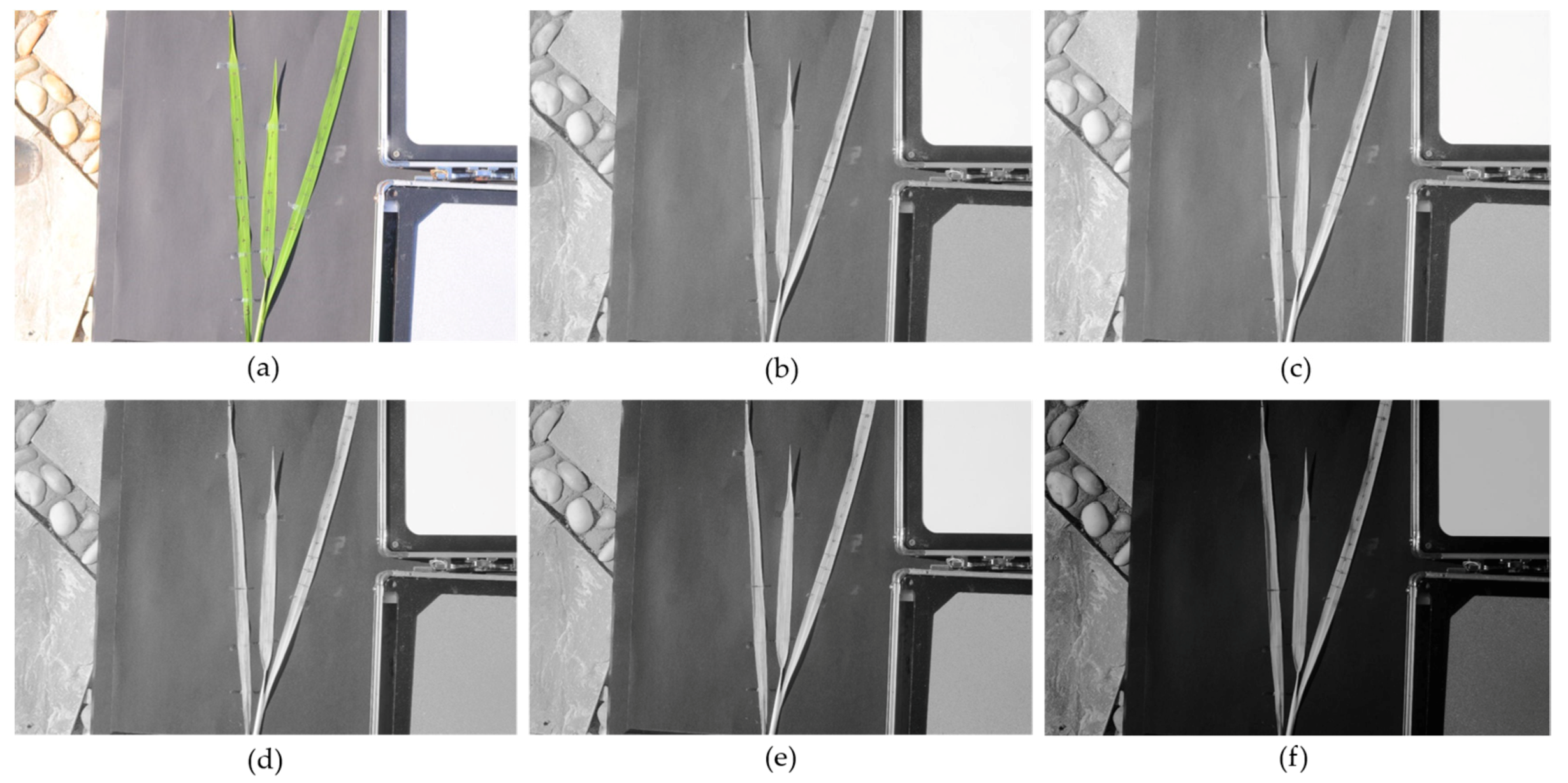
A light and miniature Rededge multispectral camera (Micasense, Inc., Fremont, CA, USA) with five imaging units was used to obtain images in blue (465–485 nm), green (550–570 nm), red (663–673 nm), NIR (820–860 nm), and red-edge (712–722 nm) bands, separately and simultaneously. The Rededge camera was carried on a small quadrotor UAV, named the Phantom 3 Advanced (DJI, Inc., Shenzhen, China), at an altitude of 40 m on 30 August 2015, in order to obtain multispectral images from field plots in a trial evaluating disease resistance in rice cultivars at the Texas A&M AgriLife Research and Extension Center, Beaumont, Texas, USA. The images shown in Figure 4, referred to as Image Set III, contained 1280 × 960 pixels and were recorded in 16-bit TIFF format.

2.1.4. Test Images

Image registration involved the alignment of a sensed image to a reference image. The sensed image needed to be transformed in order to match the reference image. Whether one image was considered as the reference depended on the number of feature points that could be selected as window centers from the image. Although only a small number of feature points could be extracted from the low contrast images, subimage pairs that were centered on such points could be very distinctive and informative. However, low contrast subimages that were centered on some feature points of a high contrast image might have contained less information. Therefore, the low contrast image should be selected as the reference image. The selection of appropriate windows and the acquisition of subimage pairs will be described in detail, later. Therefore, for Image Set I, the 650 nm, 680 nm, 720 nm, 760 nm, and 850 nm NIR images were used as reference images separately, while the RGB image was used as the sensed image. For Image Set II, the NIR image was the reference image and the RGB image was the sensed image. For Image Set III, green, red, NIR, and red-edge images were used as reference images separately, and the blue band image was used as the sensed image. All of the images were converted to grayscale images for registration.

2.2. Computer Platform and Software

Image processing was performed on a computer with an Intel Core i7, 2.60 GHz, 8.00 GB memory, and Windows 8.1 operating system. Matlab 2014 (MathWorks, Inc., Natick, MA, USA) was used for the analysis. In addition, the AutoSync module in ERDAS Imagine (Intergraph Corporation, Madison, AL, USA) and the Automatic Registration in ENVI 5.1 (Exelis Visual Information Solutions, Boulder, CO, USA) were used for comparison with the proposed method in this study.

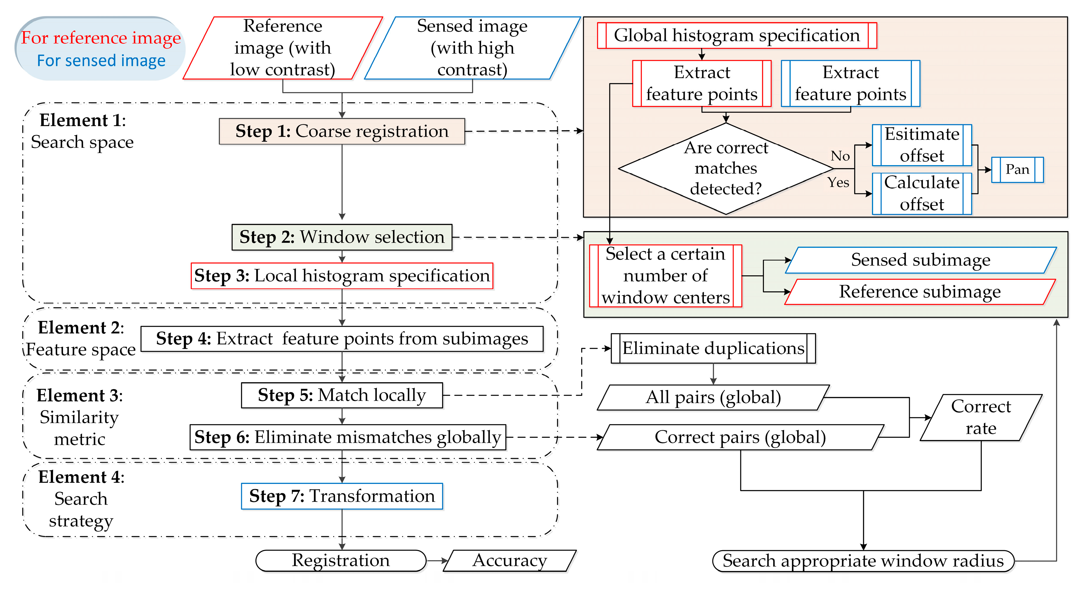
2.3. Registration Method

A widely accepted framework of an image registration algorithm, as given by Brown [26], had four standard elements, including search space, feature space, similarity metric, and search strategy. In this research, a novel registration method for optical multimodal remote sensing images was proposed. Firstly, coarse registration was applied to approximately align the sensed and reference images, window selection was used in order to reduce the search space, and histogram specification was carried out in order to optimize the similarity between the search spaces of the images. Secondly, feature points were extracted from subimages. Thirdly, a similarity metric was used to match the feature points locally, and mismatches were then eliminated globally. Lastly, a geometric transformation was applied. The specific steps are shown in Figure 5.
Step 1: Coarse registration. Using the histogram specification algorithm, the reference image with low contrast was specified to the sensed image with high contrast globally, and then an enhanced reference image was obtained. Next, the feature points were extracted from the sensed and enhanced reference images, separately. If the correct matching pairs could be detected, the average relative offset was calculated; otherwise, the approximate relative offset was estimated visually. If there was no offset, the offset was set to zero. Based on the offset, the sensed image was panned to the enhanced reference image.
Step 2: Window selection. Certain feature points of the enhanced reference image were selected as window centers. Afterwards, windows were set to be sequentially centered on these centers, so that the subimages of the reference and sensed images with the same size were prepared.
Step 3: Local histogram specification. For each set of subimages, the reference subimage with the low contrast was specified, again, to the sensed subimage with the high contrast.
Step 4: Extract feature points from subimages. Feature points were extracted from a set of subimages within the scope of the windows.
Step 5: Match locally. The matched pairs of each set of subimages within the windows were detected in turn. Afterwards, duplications from different windows were eliminated, leaving all of the matching pairs of the set of the whole images without duplications.
Step 6: Eliminate mismatches globally. False matching pairs were removed from all of the pairs of the whole images, leaving only the correct matching pairs. The correct matching rate was then calculated. Then, the optimal window radius for each image pair was searched. Considering the relationship between the optimal radius and the image width, the appropriate window radius size for any image was obtained, based on the image width.
Step 7: Transformation. By using the transformation model, which was calculated based on the coordinates of correct matching pairs, the sensed image was transformed to the reference image. The root mean square error (RMSE) was calculated to verify the accuracy of the registration.
In addition to the above steps, some key processes are explained below in more detail, including the selection of feature detectors, histogram specification, window selection, local matching, elimination of mismatches, and global transformation.

2.3.1. Selection of Feature Detectors

A selection of corresponding elements, such as pairs of good control points, in the reference and sensed images was necessary in order to determine an appropriate transformation. Lowe used the Difference of Gaussians (DoG) to find points in an image [27]. Since DoG approximated the Laplacian of Gaussian (LoG), the obtained detector behaved like the blob detector of Lindeberg [28]. Lowe named the detector that was obtained from the DoG operator SIFT, for scale-invariant feature transformation. In SIFT, a local extremum at a resolution was considered as a feature point, if its value was smaller or larger than all of its 26 neighbors in the scale space.
To find the size of a round blob, rather than tracking the extrema of the DoG or LoG, Bay et al. suggested that the locally maximum determinant of the Hessian matrix in scale space be taken and the scale at which the determinant became the maximum could be used. This detector had a repeatability that was comparable to or better than that of SIFT, while being computationally faster [29].
Curvature scale space (CSS) was proposed by Farzin Mokhtarian and Riku Suomela [30]. The first step was to extract the edges from the original image, using the Canny detector. The corner points of an image were defined as points where the image edges had their maxima of absolute curvature. The corner points were detected at a high scale of the CSS and were tracked through multiple lower scales to improve the localization.
The Harris corner detection algorithm was proposed by Chris Harris and Mike Stephens in 1988 [31]. The Harris corner detection used the moving window to calculate the change of gray values in the image. The key process included converting the images into grayscale images, calculating difference in the images, Gaussian smoothing, calculating the local extreme values, and confirming the corner points.
FAST, a fast corner feature detection operator, was proposed by Rosten and Drummond in 2006 [32]. FAST selected a pixel as a corner if the intensities of n contiguous pixels along a circle of radius 3 pixels, centered at the pixel, were all greater than the intensity of the center pixel plus a threshold value (or less than the intensity of the center pixel minus a threshold value).
In this study, the detection speed and correct matching rate of the above point detectors were compared in order to select a suitable detector, which laid the foundation for the subsequent steps of image registration.

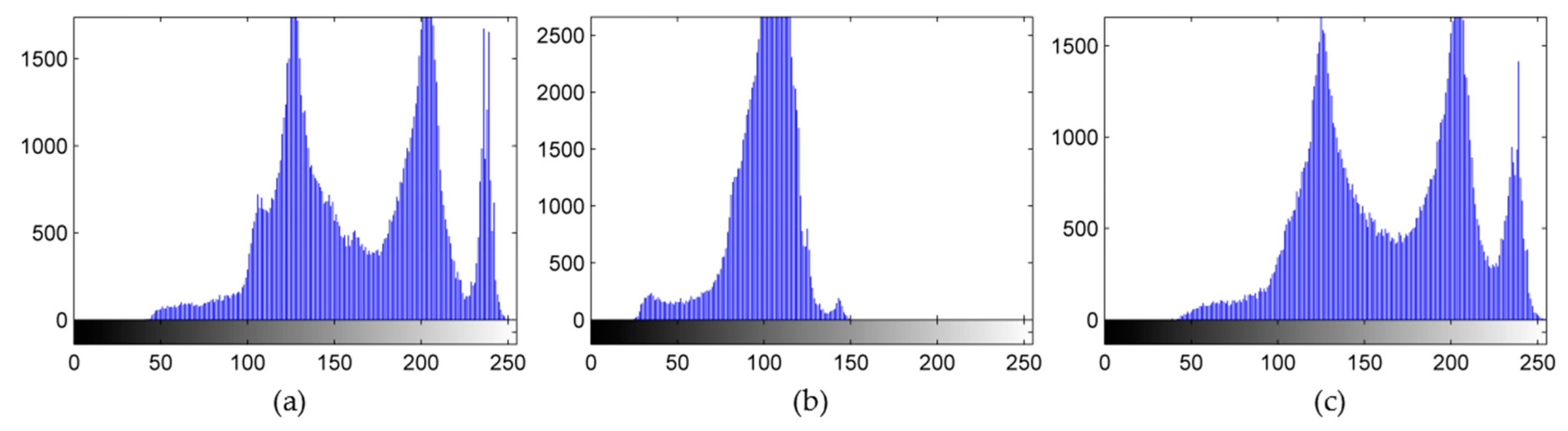
2.3.2. Histogram Specification

Histogram specification (HS) or histogram matching, as an image enhancement technique, transformed an image according to a specified gray level histogram [33]. Given two images, namely the reference image with a low contrast and the sensed image with a high contrast, their histograms were computed. The cumulative distribution functions of the histograms of the two images, F1() for the reference image and F2() for the sensed image, were calculated. Then, for each gray level G1 in the range of 0–255, the gray level G2 was found, for which F1(G1) = F2(G2), which resulted in the histogram specification function M(G1) = G2. Finally, the function M() was applied on each pixel of the reference image. HS could be used to normalize two images, when the images were acquired over the same location by different sensors.
For example, the NIR image in Local Set II had a low contrast. The low contrast of the NIR image was not conducive for feature point extraction and the low grayscale similarity was negative for subsequent matching. In order to enhance the contrast of the NIR image and increase the grayscale similarity between the NIR and RGB images, histogram specification was applied in order to convert the grayscale histogram of the NIR image into that of the RGB image, as shown in Figure 6. Clearly, the transformed histogram of the grayscale NIR image, shown in Figure 6c, had a much wider range and was very similar to the histogram of the RGB grayscale image, shown in Figure 6a. Correspondingly, the grayscale similarity between the RGB and NIR grayscale images were greatly enhanced, as shown in Figure 7.
However, the histogram processing methods mentioned above are for global transformation. The function is designed according to the gray level distribution over an entire image. Global transformation methods might not be suitable for enhancing details over small areas. The number of pixels in these small areas might have a negligible influence on designing the global transformation function. Therefore, in this study, the window selection was used. In addition to the process of coarse registration, histogram specification was applied to subimages within the windows in order to enhance local information, which greatly improved the correlation between entire multimodal images. Thus, more common points could be detected and the correct matching rate could be enhanced.

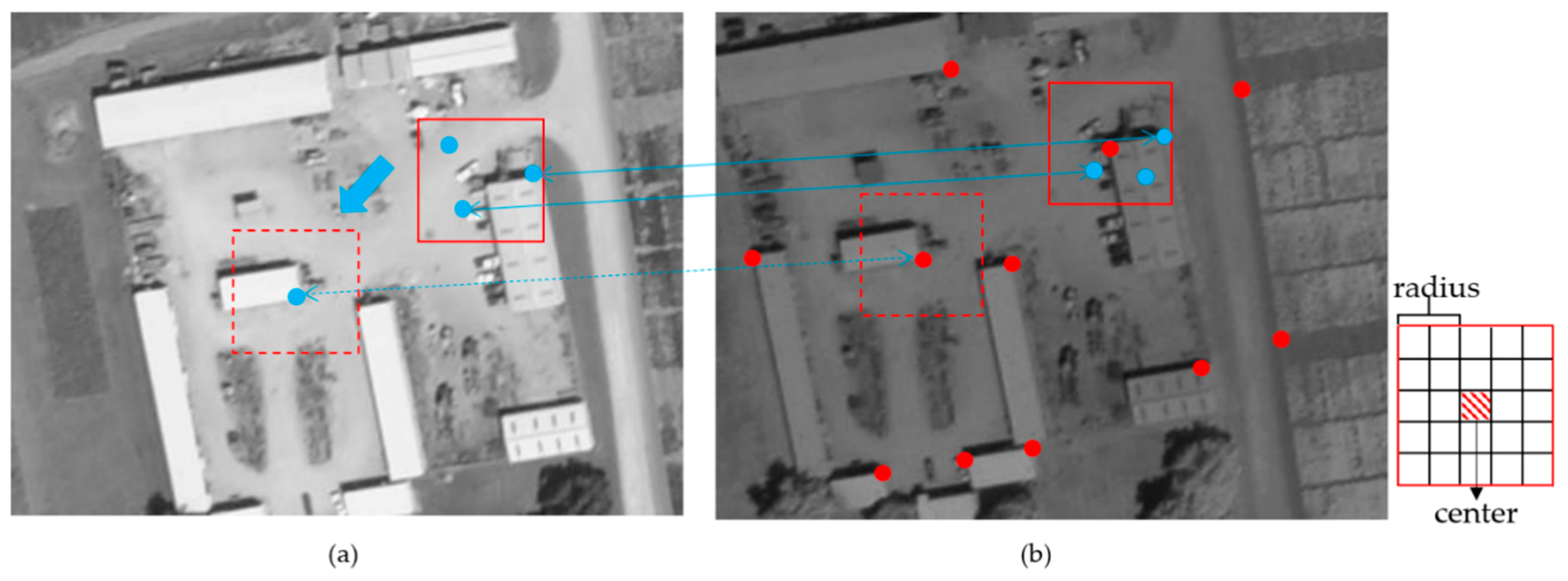
2.3.3. Window Selection and Local Matching

In the experiments, square windows were selected, with a size of (2 × radius + 1) × (2 × radius + 1). The radius was set based on the image size. After the histogram specification was applied to the reference subimage, the matching pairs were detected locally.
Much research had been conducted on algorithms for matching point features. The nearest neighbor ratio (NNR) was used to detect matching pairs. The sum of square differences (SSD) was a commonly-used distance metric function. When the distance ratio of the nearest neighbor to the second nearest neighbor was less than a certain threshold, the closest feature points were used as the matching points; otherwise, there was no matching pair. By default, the ratio was set to 0.6 in this study. A diagram of window selection and local matching is shown in Figure 8.

2.3.4. Elimination of Mismatches and Global Transformation

After duplications from the different windows were eliminated, all of the unique matching point pairs for the set of whole images were obtained. However, there were still outliers. Therefore, the false corresponding pairs were discarded by the robust estimation of the affine transformation model with an m-estimator sample consensus (MSAC) [34]. The main geometric relationship could be represented by the affine transformation model. MSAC utilized this spatial relationship in order to eliminate the false matched corner points. It was an improved version of the Random Sample Consensus (RANSAC) algorithm, which had been widely used for rejecting outliers in point matching. Both of the algorithms first estimated the affine model with three randomly selected points. Then, the transformation model was evaluated by fitting the cost function, as shown in Equation (1):
C = i ρ ( e i 2 )
where i is the number of matched corner points and ρ is the error term defined in Equation (2):
ρ ( e i 2 ) = { I , i f   e i 2 < T m T m , i f   e i 2 T m
where Tm is the threshold beyond which the matched point pairs are considered outliers for the transformation model and I is a variable that determines the difference between RANSAC and MSAC. For RANSAC, the error term is given in Equation (3):
ρ ( e i 2 ) = I = 0 ,   i f   e i 2 < T m
which means that the inliers have no effect on the estimated transformation model. For MSAC, the error term is given in Equation (4):
ρ ( e i 2 ) = I = e i 2 ,   i f   e i 2 < T m
which means that every inlier has a different impact on the cost function that is used for defining a transformation model [35]. By default, the number of maximum random trails was set to 1000 for finding the inliers, and the confidence of finding maximum number of inliers was set to 0.99. Furthermore, the maximum distance in pixels, from a point to the estimated transformation of its corresponding point, was set to 1.5.
A transformation function that used the coordinates of the corresponding control points identified in two images in order to estimate the geometric relation between the images, which was then used to transform the geometry of the sensed image to that of the reference, in order to spatially align the images. There were some deformations between optical multimodal remote sensing images, such as translation, rotation, scaling, shearing, or any combination of these. Therefore, an affine geometric transformation was adopted. In this process, the point matrix in the reference image is p = f (x, y, z), and that of the sensed image is q = F (x′, y′, z′). The relation between the two images is p = H · q, and H is a 3 × 3 matrix [36], as shown in Equation (5):
p = [ x y z ] = [ h 11 h 12 h 13 h 21 h 22 h 23 h 31 h 32 h 33 ] · [ x y z ] = [ h 1 T h 2 T h 3 T ] · [ x y z ] = H · q
where hij (i = 1, 2, 3; j = 1, 2, 3) are elements of H and hi (i = 1, 2, 3) is (hi1, hi2, hi3). For the affine transformation, h31 = h32 = 0, and h33 = 1.

3. Results

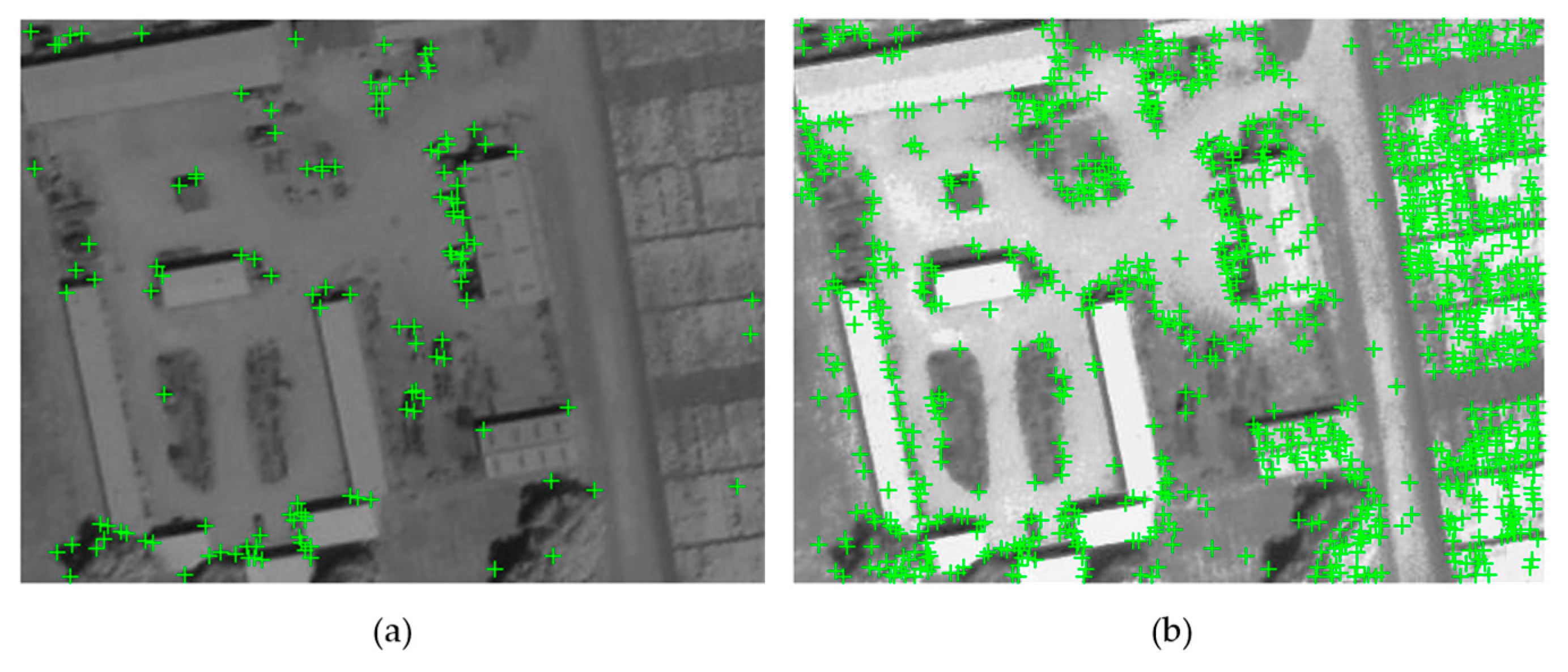
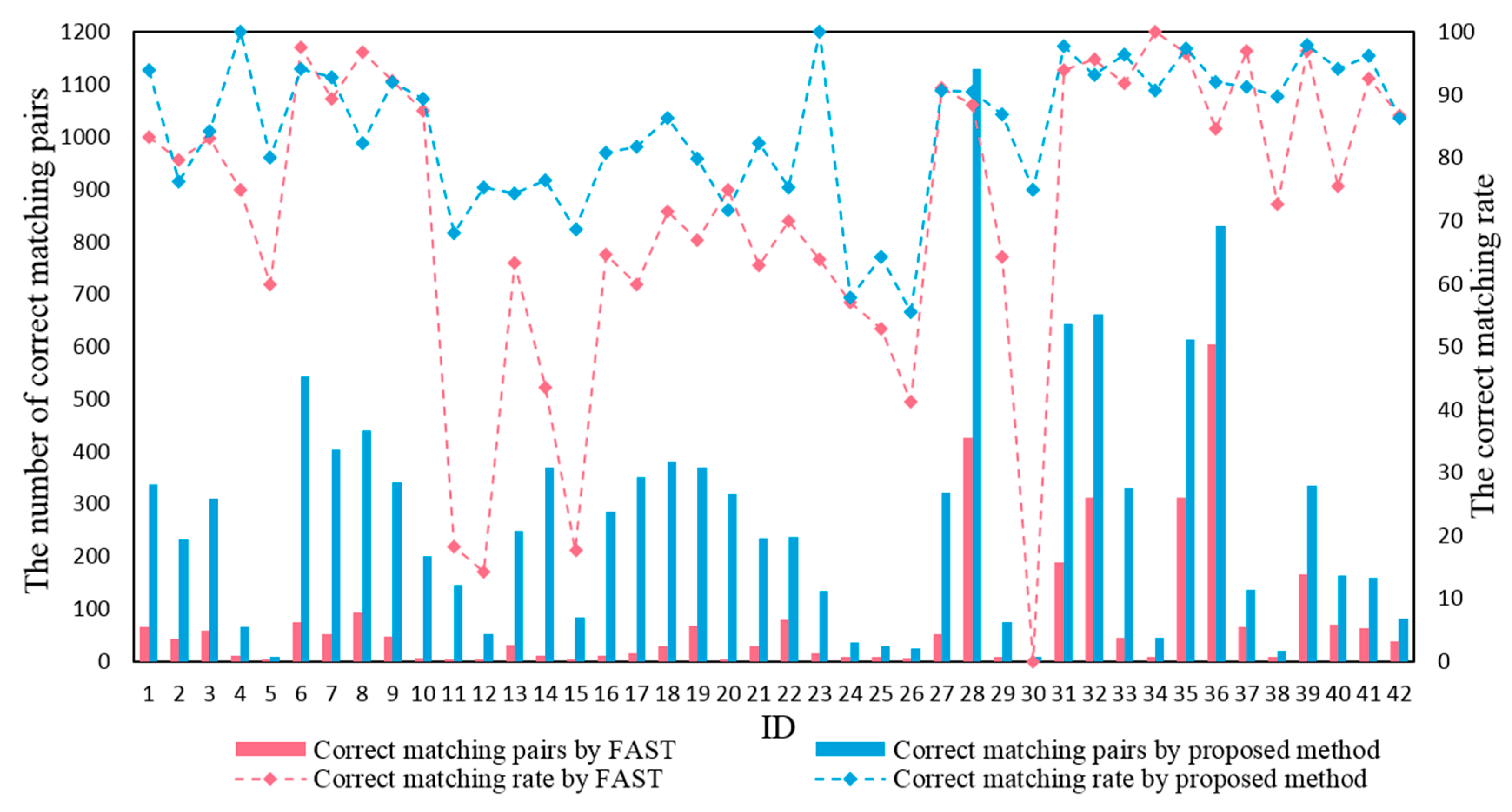
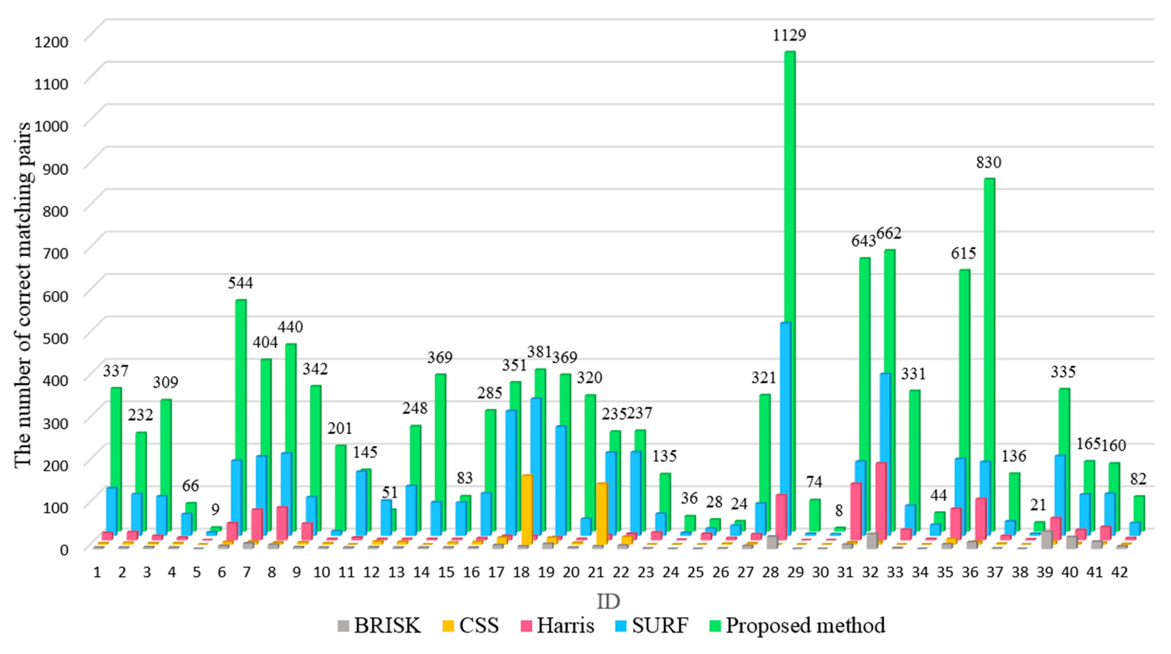
3.1. Comparison of Feature Detectors

Using the reference and sensed images in Local Image Set II with 400 × 300 pixels as an example, five different detection algorithms, including SIFT, CSS, Harris, SURF, and FAST, were used to extract the feature points for matching this set of images. In order to compare the correct matching rate of different detection algorithms under the same standard, the parameters of the feature detectors were adjusted so that a similar number of corner points were extracted. NNR was applied to detect the matching pairs and MSAC was used to eliminate the outliers. The detection speed and correct matching rate were calculated. Table 1 presents the matching results for the five detectors.
As shown in Table 1, the advantages of FAST were its rapid detection speed and high correct matching rate, however the number of correct matching pairs needed to be further increased. SIFT had the highest correct matching rate, which was only 0.50% higher than FAST, however its detection speed was the slowest, and the number of correct matching pairs was about the same as it was for FAST. For SURF, the number of correct matching pairs was the highest, however its correct rate was the lowest. Therefore, FAST was selected to detect the feature points in this study, considering the intensive computations that were required for the remote sensing images. As shown in Figure 9, the registration result was acceptable, with a good overlap and relatively uniform point distribution. In addition to the use of the FAST algorithm, a method based on the histogram specification within the windows was proposed, in order to increase the number of correctly matched pairs, and to enhance the correct matching rate.

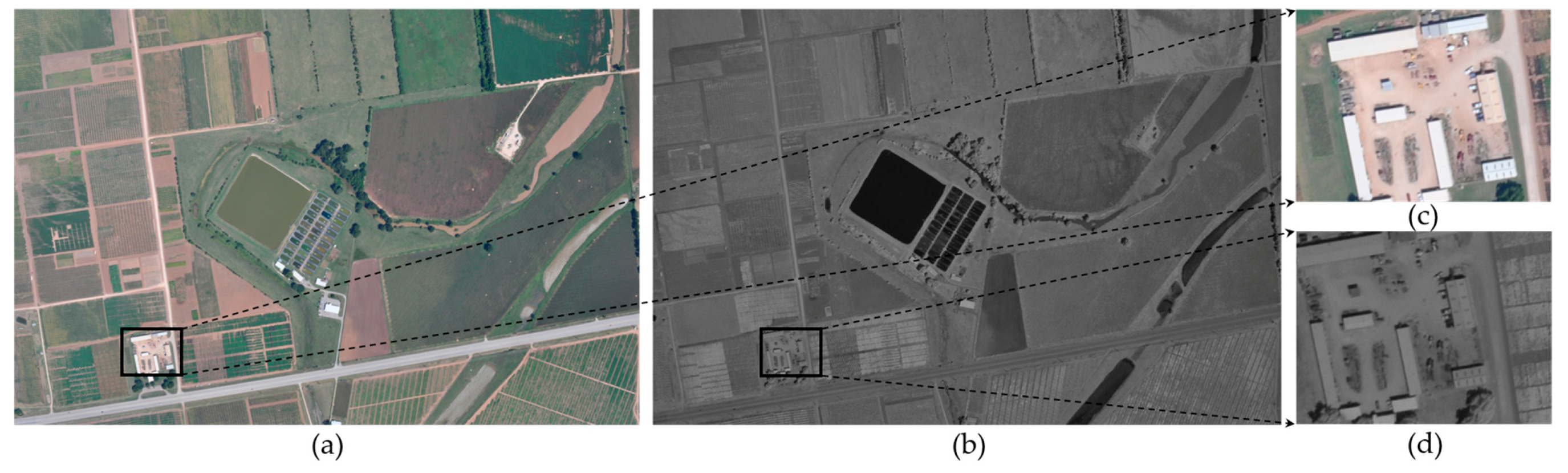
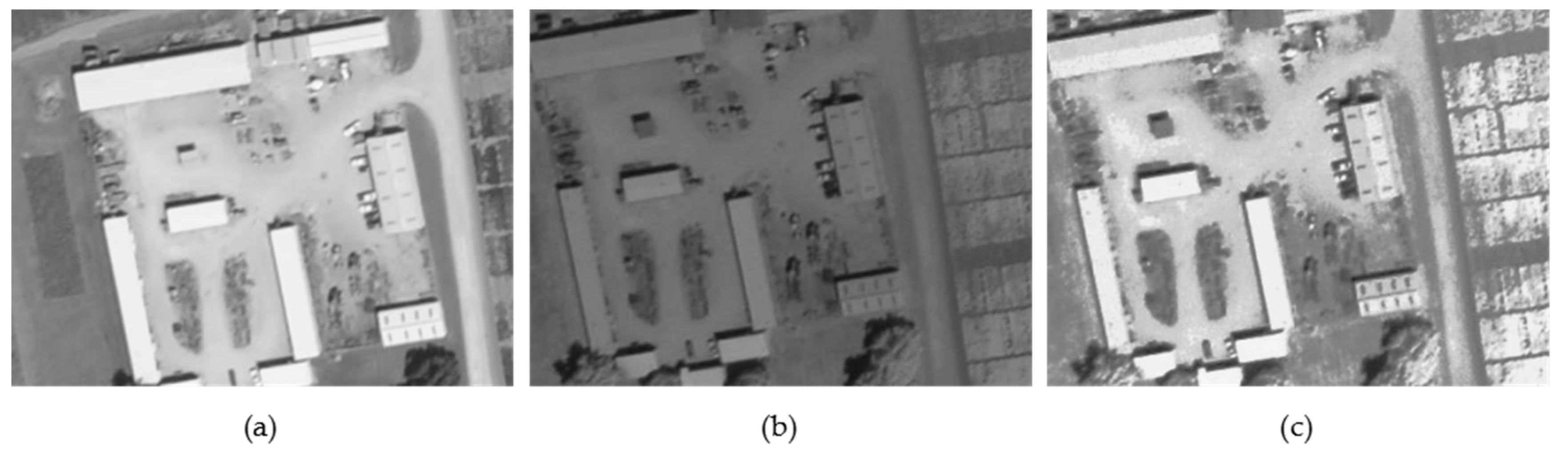
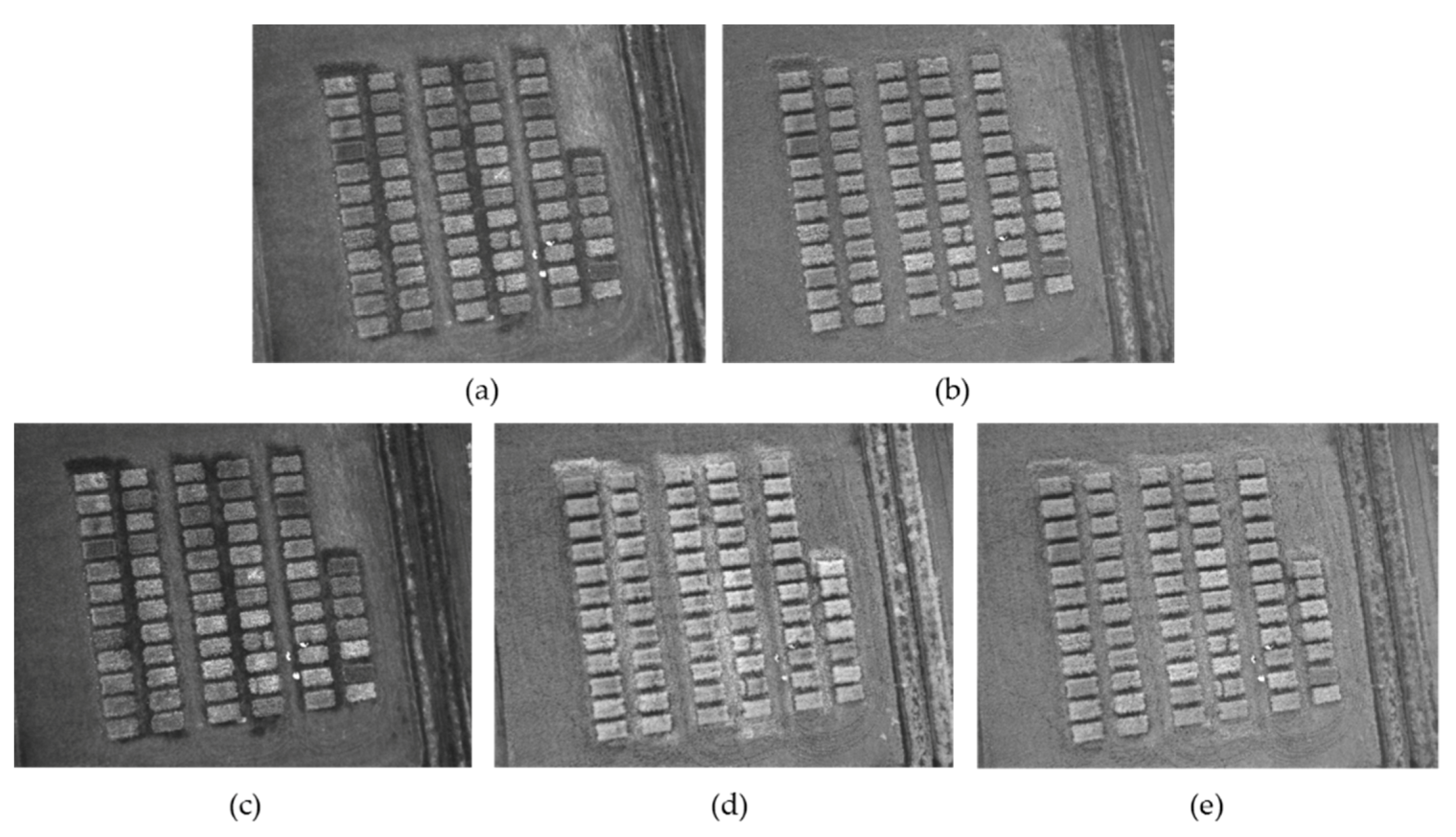
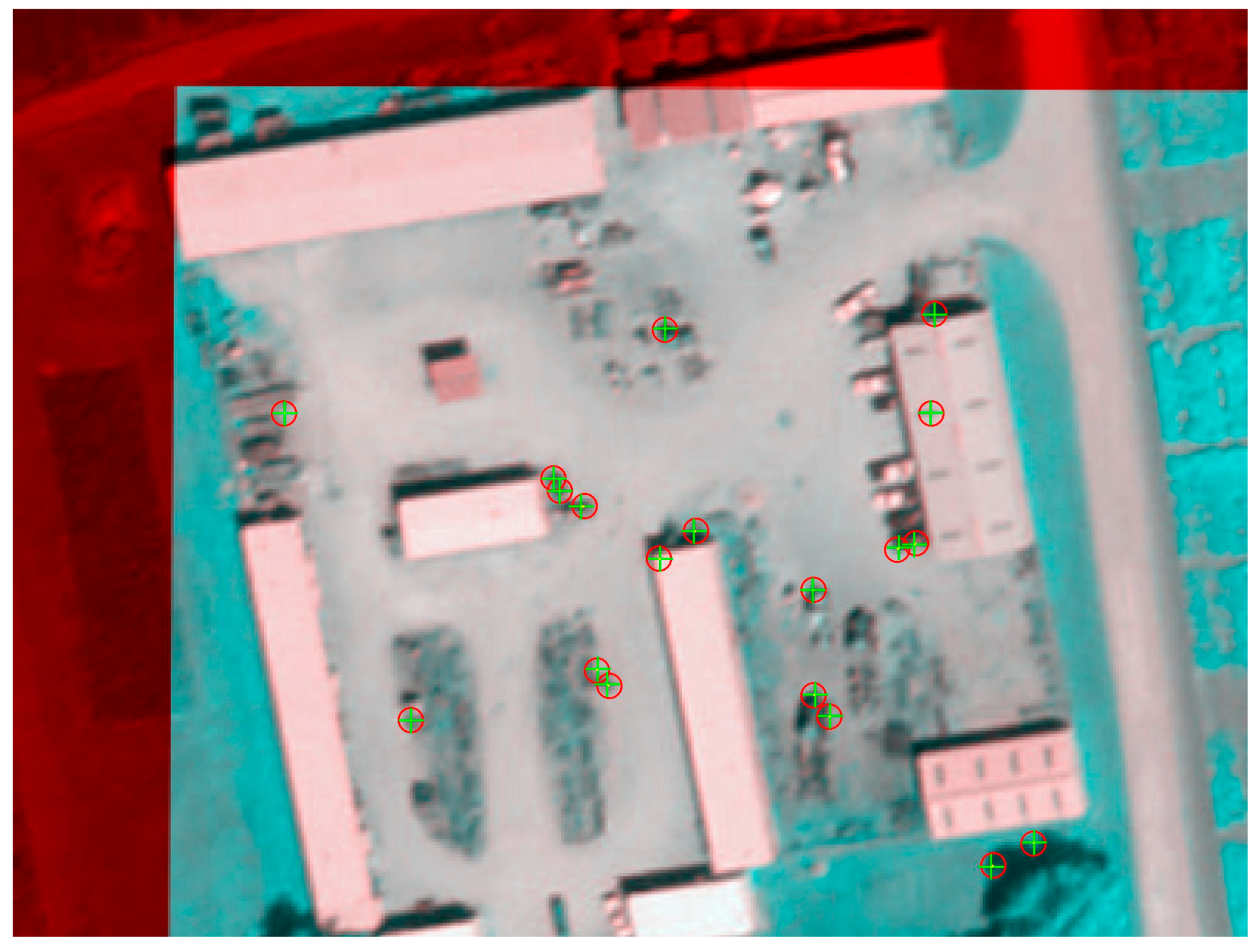
3.2. Registration Result

One set of optical multimodal remote sensing images acquired by each of the three types of imaging sensors were tested using the proposed registration method, based on FAST, window selection, and histogram specification. Firstly, it was essential to search the optimal window radius for each set of images. By adjusting the minimum accepted quality of the FAST corner points, the number of the window centers of the reference image was controlled at about 200, and the registration time was set to be less than 30 s, which resulted in relatively uniform window centers and similar conditions for the subsequent window size comparison. Figure 10 shows the trend graphs of the numbers of all of the matching pairs and the correct matching pairs for the different window radiuses.
With the increase of the window radius, the number of all of and the correct matching pairs sharply increased, and then flattened after reaching certain values. The larger the window size, the more repetitive pairs were detected. Therefore, windows larger than an optimal size did not greatly increase the number of the correct matching pairs, but used more computing time. The optimal window radius depended on the actual size and content of the images. Generally, there were more matching pairs between images with similar wavelengths, such as visible images. For the same window size, more matching pairs were detected from the Local Set II than from the Global Set II, because there were richer image content and more landmarks in the Local Set II images.
Figure 11 shows the trend graphs of the correct matching rate for the different window radiuses. The correct matching rate decreased with the increase of the window radius. This result demonstrated that the smaller windows tended to have a higher correct matching rate. Furthermore, for the registration between the visible images, the correct matching rate was high and was only slightly affected by the size of the window. However, for registration between the visible and NIR images, the larger the difference in the image wavelengths, the lower the correct matching rate.

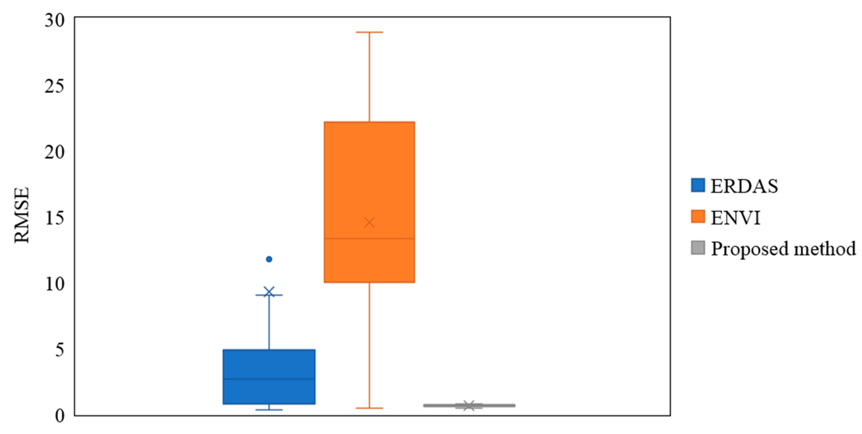
3.3. Accuracy Assessment

As a result of the differences in grayscale image content, the image registration accuracy varied. Nevertheless, the RMSE in the x and y directions was generally within 0.5 pixels, as shown in Figure 12. This accuracy was sufficient for the registration of optical multimodal remote sensing images. The registration method, based on FAST, window selection, and histogram specification, was accurate and feasible for practical applications.

4. Discussion

Since all of the bands of the commonly-used multispectral cameras with frame sensors had different spectral ranges, it was difficult to identify the common feature points among the band images, especially between the visible and NIR bands. The proposed method, based on FAST detection, window selection, and histogram specification, could increase the number of the correct matching pairs and improve the registration accuracy, by reducing the search space and optimizing the feature similarity. The simple method with a rapid detection speed was useful for the registration of remote sensing images, because of their characteristic of being computationally intensive. To further verify the universality and effectivity of the proposed method, Set I-b, c, d; Set II-b, c, d; and Set III-b, c, d were added. The search for the appropriate window radius size, which was an important parameter, was discussed first in this section. Based on the appropriate window radius size, the importance of the histogram specification within the windows was discussed, and the proposed method was then compared with the commonly-used methods. The discussion and comparison should have provided useful information for other research studies of the multimodal remote sensing images registration methods.

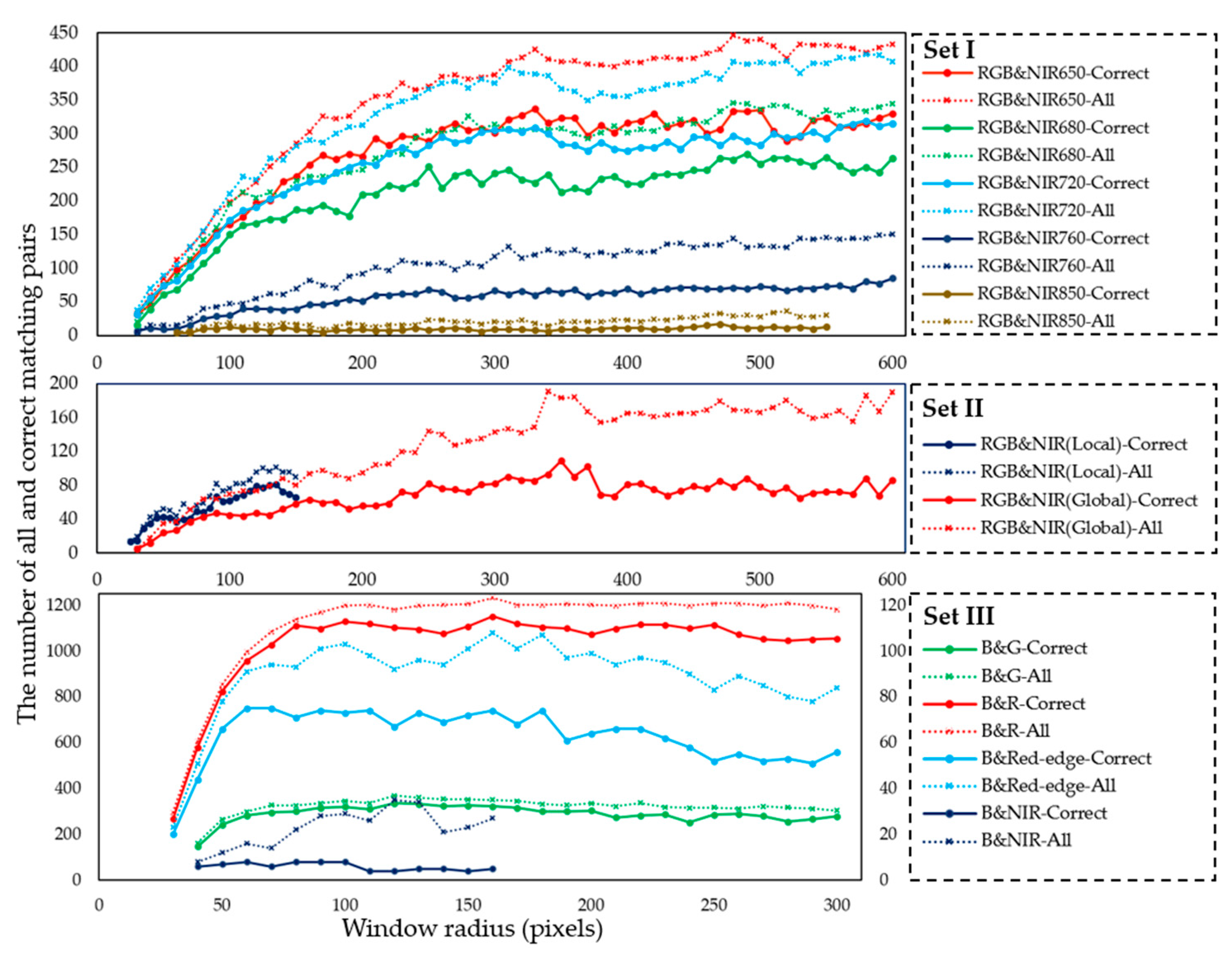
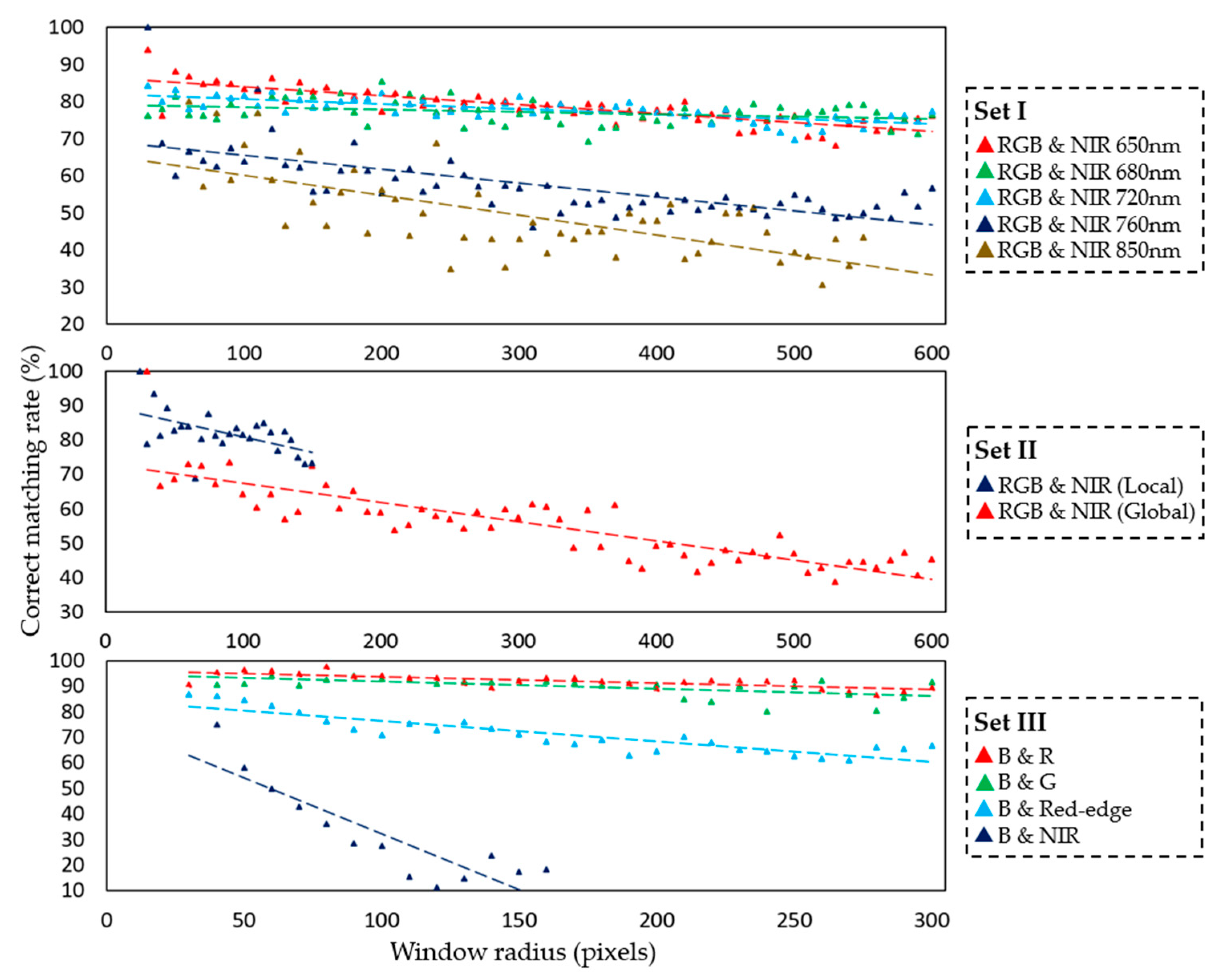
4.1. Search for the Appropriate Window Radius Size

The optimal window radius size depended on the actual size and content of the images. It was not feasible to get the best registration result for a set of images by constantly setting different values of the window radius size, which was time-consuming. Therefore, it was necessary to search for an appropriate radius size for each type of the images. As shown in Table 2, we discovered that the optimal radius size was about one-tenth of the image width. Therefore, the window radius size in the proposed method should have been set to one-tenth of the image width. Then, the appropriate window radius size of each image set was calculated for the subsequent comparison.

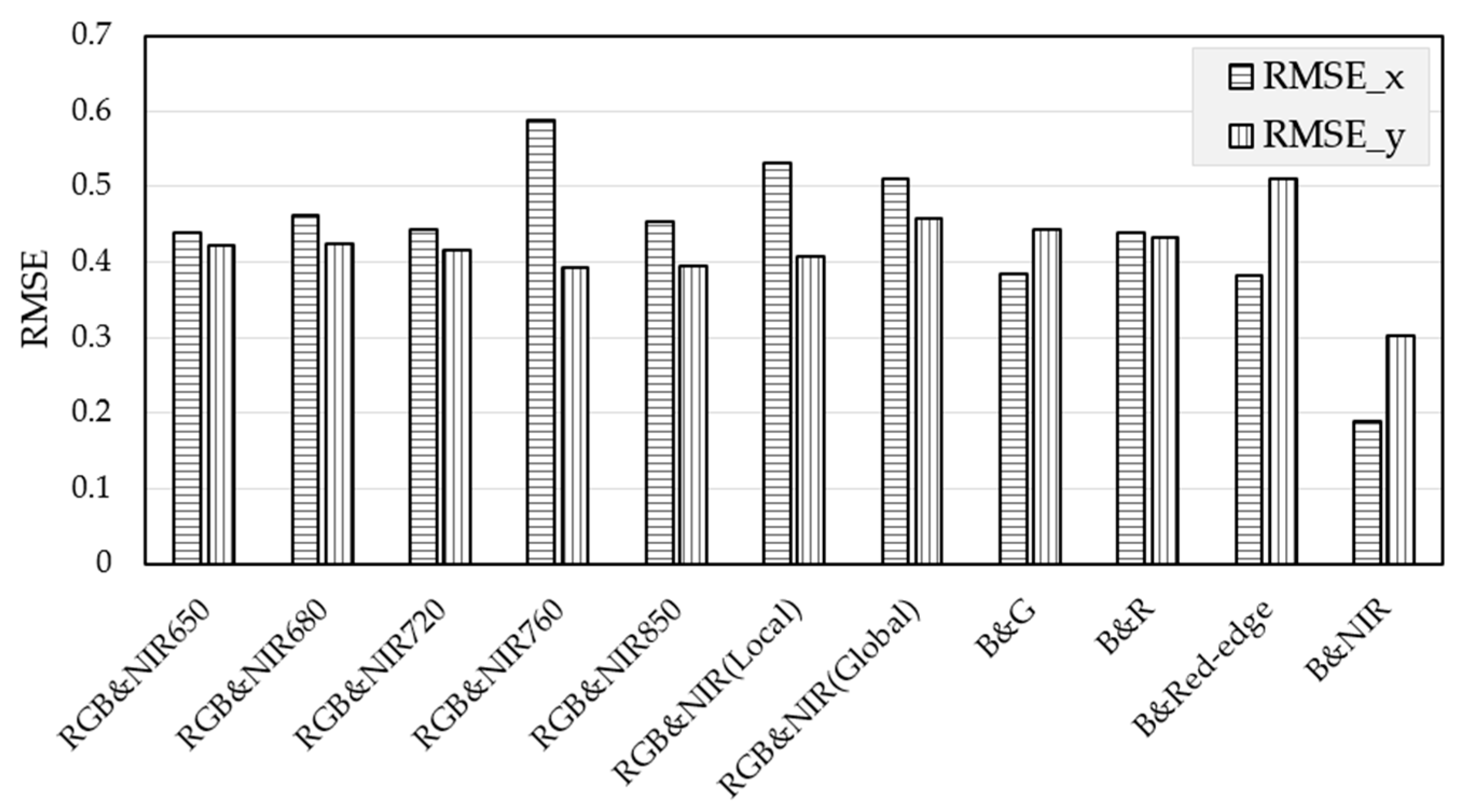
4.2. Importance of Histogram Specification within Windows

Firstly, in order to verify the effect of the histogram specification, the FAST algorithm parameters remained unchanged in this comparison experiment, where the minimum accepted quality of the corners remained 0.01 and the minimum intensity remained 0.1. A total of 126 feature points from the initial NIR grayscale image were extracted by FAST, as shown in Figure 13a. In contrast, 1163 feature points were extracted from the transformed NIR grayscale image with the histogram specification, as shown in Figure 13b. This result revealed that the histogram specification could significantly increase the number of feature points in the image with the low contrast. Furthermore, the gray value similarity between the NIR and RGB images was improved for effective matching of the feature points. Obviously, if the histogram specification was applied on subimages, the gray value similarity between the multimodal images would increase.
Based on the appropriate window radius size calculated previously for each image set, the number of the correct matching pairs and the correct matching rate using FAST, window selection, and histogram specification were determined and compared with the matching results that were based on FAST, only to highlight the effect of the histogram specification within the windows (Figure 14).
It can be seen from Figure 14 that the number of correct matching pairs increased significantly and the correct matching rate also improved with the window selection and histogram specification compared with FAST alone. On average, the number of correct matching pairs had increased by 11.30 times and the correct matching rate had increased by 36%, compared with those based on FAST only. As a result of the similarity of the grayscale contrast between visible images, the original FAST method alone was sufficient. Nevertheless, the proposed method had also improved the matching results on the visible images. Furthermore, the method was especially suitable for the registration between the visible and NIR images. In particular, the registration between the blue and NIR images of Set III-a (ID30) achieved a breakthrough. The number of matching pairs increased from 0 to 8, and the matching rate increased from 0 to 75%. These results showed that histogram specification within the windows was effective because it increased the number of correct matching pairs and enhanced the correct matching rate, on the basis of the FAST detector.
Since the sensed and reference images had a large overlap, a simple translation made the content of a pair of subimages more consistent. On the basis of this, the window selection reduced the corresponding feature search space so as to effectively minimize the possibility that two or more similar feature points in one image would incorrectly match the same point in the other image. Therefore, the window selection had reduced the time needed to eliminate the wrong matching pairs and improved the matching speed. The histogram specification that was applied with windows, enhanced the grayscale similarity between the sensed and reference subimages. Therefore, the histogram specification in conjunction with the window selection was very effective in the registration of optical multimodal remote sensing images.

4.3. Comparison of State-Of-The-Art Methods and the Proposed Method

Figure 15 compares the numbers of correct matching pairs of the binary robust invariant scalable keypoints (BRISK), CSS, Harris, and SURF, with those of the proposed method. BRISK had a dramatically lower computational cost (an order of magnitude faster than SURF in cases). The key to high speed lay in the application of a scale-space FAST-based detector in combination with the assembly of a bit-string descriptor, from intensity comparisons that were retrieved by a dedicated sampling of each keypoint neighborhood. However, the performance of BRISK was poor. CSS was robust with respect to noise and scale, and was more effective for applications such as shape retrieval, object recognition, and corner detection, however it had a poor performance, with deep and shallow concavities of the shape, and failed to address the problem of the open curves that were present in the given shape. The Harris corner detection operator had a rotation invariance but no scale invariance. SURF was considered as the most computationally efficient among all of the high-performance methods to date. It exhibited great performance under a variety of image transformations, but it was not very suitable for optical multimodal remote sensing images. It was clear that the number of correct matching pairs of the proposed method was significantly larger than the other methods. The effectivity of the proposed method benefited from the high detection speed of the FAST feature detector, the appropriate window size to limit the scope of image registration, and the histogram specification in order to improve the grayscale similarity between the subimages within the windows.

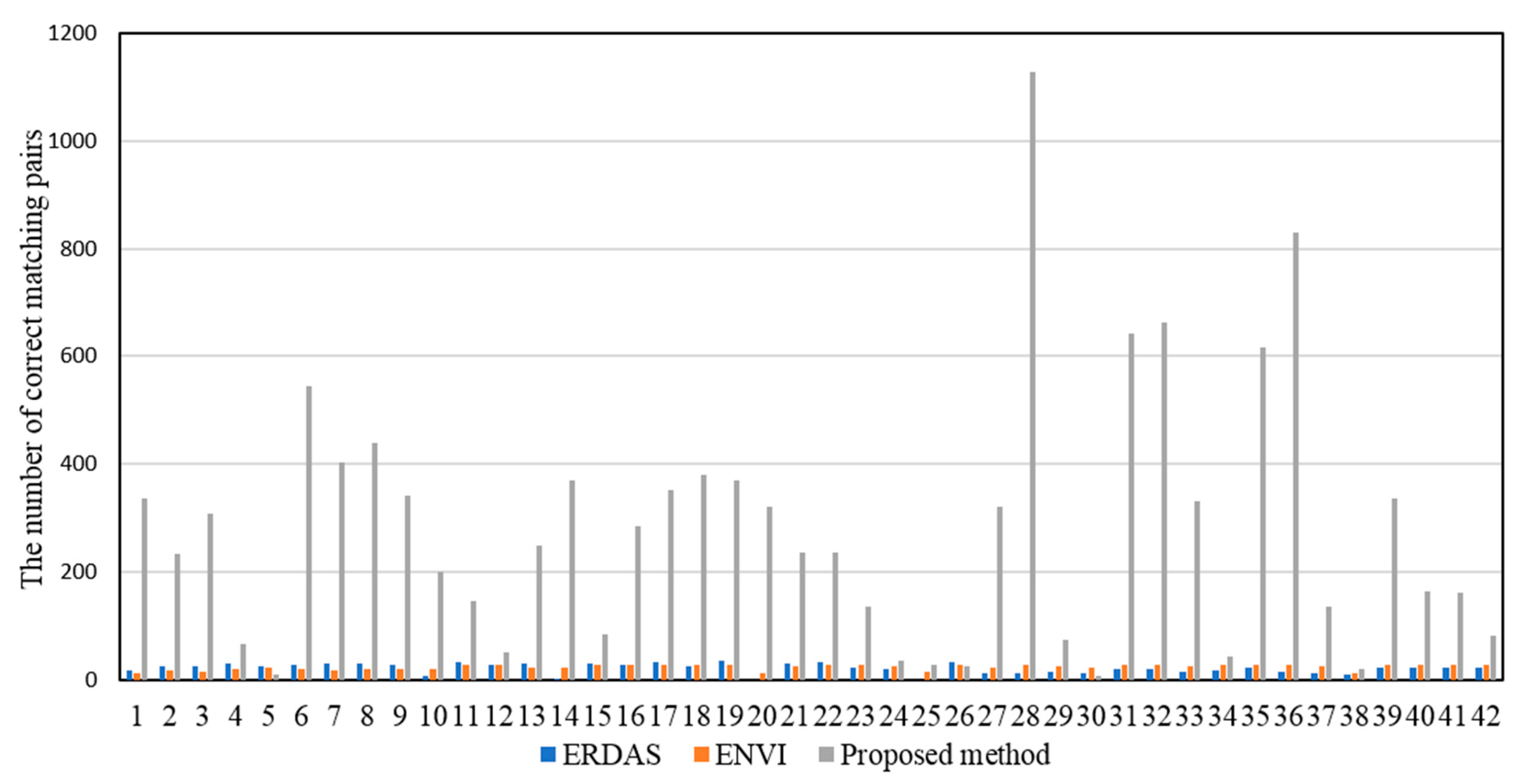
4.4. Comparison of Software Embedded Methods and the Proposed Method

To further demonstrate the validity, the registration results of the proposed method were compared with those of the AutoSync module in ERDAS Imagine and the Automatic Registration in ENVI. The 12 sets of multimodal remote sensing images were registered separately, using the AutoSync module in the ERDAS Imagine. The image with the low contrast was chosen as the reference image, so as to be consistent with the tests of the proposed method. Since AutoSync required a minimum of three points to perform an automatic point measurement on the images with no coordinate system information, three tie control points were chosen manually before the automatic registration. Default parameters were used and new tie points were generated by AutoSync automatically. Automatic Registration in ENVI was used to align the 12 sets of images. Similarly, the image with the low contrast was chosen as the reference image and three tie control points were chosen manually before the automatic registration.
From Figure 16, the numbers of correct matching pairs for the proposed method were much larger than those for ENVI, except for one case and, for ERDAS, except for two cases. The sensed and reference images for the three cases had very different electromagnetic wavelengths and most of the matching pairs occurred in relatively homogeneous areas by ERDAS and ENVI, which might not have been accurate. Moreover, the difference in the image pairs between the software embedded methods and the proposed method was small for the three cases. In tests 20 and 25, the ERDAS AutoSync had the following warning, “The contrast of image is very low and it may cause undesirable results, resulting in the inability to register for image pairs”. Therefore, the proposed method could have greatly increased the number of the correct matching pairs and was more effective.
The registration accuracy of the proposed method was accurate and consistent, as shown in Figure 17. The RMSE values of the proposed method were smaller than those of ENVI, except for one case, and for ERDAS, except for five cases. As for the six cases, the correct matching pairs that were extracted by ERDAS and EVNI were far from enough, so the registration accuracy was compromised. However, the numbers of the correct matching pairs of the proposed method were much larger than those of ERDAS and ENVI, and the RMSE values of the proposed method were similar to those of ERDAS and ENVI.
There were several reasons for the better results from the proposed method than from ERDAS and ENVI. Firstly, the quality of the input data for the AutoSync module in ERDAS played a crucial role in determining the registration accuracy and extent of the user intervention that was required. For good automatic point measurement (APM) performance, the same band or a similar band in the images for point matching should have been selected, to ensure similarity of radiometric characteristics. Infrared bands should have generally been avoided [37]. However, input and reference images could differ greatly in the electromagnetic wavelengths for optical multimodal remote sensing images registration.
Secondly, being non-isotropic was one of the main problems with Moravec, the interest operator in ENVI. If an edge was present that was not in the direction of the neighbors (horizontal, vertical, or diagonal), then the small SSD would be large and the edge would be incorrectly chosen as an interest point. However, for FAST in the proposed method, the intensities of the contiguous pixels along a circle with a radius of 3 that was centered at the interest point, were considered.
Thirdly, based on the default distribution, the APM collected matching points within a fixed area of 512 × 512 pixels, which were centered on the corresponding grid intersection of each image. AutoSync searched for the corresponding point within a 17 × 17 pixel square window. For ENVI, the 81× 81 pixel search window was a defined subset of the image, within which the smaller 11 × 11 pixel moving window scanned to find a feature match for a tie point placement [38]. However, the fixed window size and location might not have been suitable for the multimodal remote sensing images. In the proposed method, the appropriate window size was varied from the actual image size and the windows were centered on a certain number of the feature points that extracted in the coarse registration. The subimage pairs that were centered on such points were generally very distinctive and informative, which resulted in an appropriate feature search space and more feature points.
Fourthly, the low contrast and grayscale similarity could have led to only a few or no correct matching points within some of the less distinctive grids, thus wasting time. The actual number of the corresponding points that were extracted was far less than the default intended number of points in ERDAS and ENVI. Therefore, in order to identify sufficient match points for different scenes, it was necessary to manually and constantly adjust the minimum point match quality, correlation size, and least squares size for ERDAS, as well as the area chip size, minimum correlation, and point oversampling for ENVI. The adjustments of these parameters did not improve the grayscale similarity between the image pairs. In the proposed method, the feature similarity could be locally optimized by the histogram specification within the windows, which contributed to more correct matching pairs and a higher correct matching rate. Moreover, no initial points needed to be manually selected using the method so as to avoid operational uncertainty and reduce adverse effects on subsequent analysis.
Although ERDAS and ENVI, two of themost commonly-used image processing software packages, had flexible user interfaces and registration modules, they were not as effective as the proposed method was for the registration of optical multimodal remote sensing images. The proposed method employed a combination of FAST, window selection, and histogram specification in order to deal with the differences in the spectral response of sensors and the low correlations in grayscale values between the sensed and reference images.

5. Conclusions

In this research, a novel method was proposed for the registration of optical multimodal remote sensing images, based on FAST detection, window selection, and histogram specification. The commonly-used multispectral cameras with digital frame sensors were used to acquire RGB, red-edge, and NIR images. The image analysis showed that the FAST detector with a rapid processing speed was suitable for extracting feature points for subsequent point matching. Since the window selection reduced the search space and the histogram specification optimized the feature similarity, the combination of these two techniques made the number of correctly matched point pairs increase by 11.30 times and the correct matching rate increase by 36%, compared with the results based on FAST alone.
As the window radius increased, the number of all of and the correct matching pairs sharply increased and then flattened. There were more matching pairs between the images with similar wavelengths or the images with a richer content and more obvious structure. Smaller windows tended to increase the correct matching rate. The appropriate window radius was thoroughly searched and set to one-tenth of the image width in the proposed method. Furthermore, the RMSE values in x and y directions were generally within 0.5 pixels for the proposed method. This accuracy was sufficient for the registration of optical multimodal remote sensing images. The proposed method performed generally better than the other state-of-the-art methods and the automatic registration modules built in ERDAS and ENVI. In addition, there was no need to manually select any initial points in the proposed method before registration.
Future research is needed to refine the method proposed in this study for specific applications, so that it can be used for the registration of optical multimodal remote sensing images. More research is also needed in order to evaluate the window selection and histogram specification, with FAST and other detectors, for registering the remote sensing images and other spatial data, such as Lidar.

Author Contributions

Xiaoyang Zhao designed the method, conducted the experiment, analyzed the data, discussed the results and wrote the majority of the manuscript. Jian Zhang contributed to the method design, participated in sensor testing and image collection, provided test data, advised in data analysis, and wrote a part of the manuscript. Chenghai Yang guided the study design, advised in data analysis, and revised the manuscript. Huaibo Song contributed to the method design and discussed the results. Yeyin Shi, Xin-Gen Zhou, Dongyan Zhang, and Guozhong Zhang were involved in the process of the experiment, ground data collection, or manuscript revision. All authors reviewed and approved the final manuscript.

Acknowledgments

This project was financially supported by the National Natural Science Foundation of China (Grant No. 41201364 and 31501222), the Fundamental Research Funds for the Central Universities (Grant No. 2662017JC038) and the Innovation Training Plan Program of University Student (Grant No. 201610504017).

Conflicts of Interest

The authors declare no conflict of interest.

References

  1. Aicardi, I.; Nex, F.; Gerke, M.; Lingua, A. An image-based approach for the co-registration of multi-temporal uav image datasets. Remote Sens. 2016, 8, 779. [Google Scholar] [CrossRef]
  2. Pritt, M.; Gribbons, M.A. Automated Registration of Synthetic Aperture Radar Imagery with High Resolution Digital Elevation Models. U.S. Patent No. 8,842,036, 23 September 2014. [Google Scholar]
  3. Tommaselli, A.M.; Galo, M.; De Moraes, M.V.; Marcato, J.; Caldeira, C.R.; Lopes, R.F. Generating virtual images from oblique frames. Remote Sens. 2013, 5, 1875–1893. [Google Scholar] [CrossRef]
  4. Chen, J.; Luo, L.; Liu, C.; Yu, J.-G.; Ma, J. Nonrigid registration of remote sensing images via sparse and dense feature matching. J. Opt. Soc. Am. A 2016, 33, 1313–1322. [Google Scholar] [CrossRef] [PubMed]
  5. Turner, D.; Lucieer, A.; de Jong, S. Time series analysis of landslide dynamics using an unmanned aerial vehicle (UAV). Remote Sens. 2015, 7, 1736–1757. [Google Scholar] [CrossRef]
  6. Sedaghat, A.; Ebadi, H. Remote sensing image matching based on adaptive binning sift descriptor. IEEE Trans. Geosci. Remote Sens. 2015, 53, 5283–5293. [Google Scholar] [CrossRef]
  7. Grant, B.G. UAV imagery analysis: Challenges and opportunities. In Proceedings of the Long-Range Imaging II, Anaheim, CA, USA, 1 May 2017; Volume 10204, p. 1020406. [Google Scholar]
  8. Zhang, J.; Yang, C.; Song, H.; Hoffmann, W.; Zhang, D.; Zhang, G. Evaluation of an airborne remote sensing platform consisting of two consumer-grade cameras for crop identification. Remote Sens. 2016, 8, 257. [Google Scholar] [CrossRef]
  9. Kelcey, J.; Lucieer, A. Sensor correction and radiometric calibration of a 6-band multispectral imaging sensor for uav remote sensing. Int. Arch. Photogramm. Remote. Sens. Spat. Inf. Sci. 2012, 39-B1, 393–398. [Google Scholar] [CrossRef]
  10. Dehaan, R. Evaluation of Unmanned Aerial Vehicle (UAV)-Derived Imagery for the Detection of Wild Radish in Wheat; Charles Sturt University: Albury-Wodonga, Australia, 2015. [Google Scholar]
  11. Bongiorno, D.L.; Bryson, M.; Dansereau, D.G.; Williams, S.B. Spectral characterization of COTS RGB cameras using a linear variable edge filter. Korean J. Chem. Eng. 2013, 8660, 618–623. [Google Scholar]
  12. McKee, M. The remote sensing data from your UAV probably isn’t scientific, but it should be! In Proceedings of the Autonomous Air and Ground Sensing Systems for Agricultural Optimization and Phenotyping II, Anaheim, CA, USA, 8 May 2017; Volume 10218, p. 102180M. [Google Scholar]
  13. Zitova, B.; Flusser, J. Image registration methods: A survey. Image Vis. Comput. 2003, 21, 977–1000. [Google Scholar] [CrossRef]
  14. Joglekar, J.; Gedam, S.S. Area based image matching methods—A survey. Int. J. Emerg. Technol. Adv. Eng. 2012, 2, 130–136. [Google Scholar]
  15. Moigne, J.L.; Netanyahu, N.S.; Eastman, R.D. Image Registration for Remote Sensing; Cambridge University Press: Cambridge, UK, 2011. [Google Scholar]
  16. Hong, G.; Zhang, Y. Combination of feature-based and area-based image registration technique for high resolution remote sensing image. In Proceedings of the IEEE International Geoscience and Remote Sensing Symposium, Barcelona, Spain, 23–28 July 2007; pp. 377–380. [Google Scholar]
  17. Behling, R.; Roessner, S.; Segl, K.; Kleinschmit, B.; Kaufmann, H. Robust automated image co-registration of optical multi-sensor time series data: Database generation for multi-temporal landslide detection. Remote Sens. 2014, 6, 2572–2600. [Google Scholar] [CrossRef]
  18. Habib, A.F.; Alruzouq, R.I. Line-based modified iterated Hough transform for automatic registration of multi-source imagery. Photogramm. Rec. 2004, 19, 5–21. [Google Scholar] [CrossRef]
  19. Sheng, Y.; Shah, C.A.; Smith, L.C. Automated image registration for hydrologic change detection in the lake-rich Arctic. IEEE Geosci. Remote Sens. Lett. 2008, 5, 414–418. [Google Scholar] [CrossRef]
  20. Shah, C.A.; Sheng, Y.; Smith, L.C. Automated image registration based on pseudoinvariant metrics of dynamic land-surface features. IEEE Trans. Geosci. Remote Sens. 2008, 46, 3908–3916. [Google Scholar] [CrossRef]
  21. Lowe, D.G. Distinctive image features from scale-invariant keypoints. Int. J. Comput. Vis. 2004, 60, 91–110. [Google Scholar] [CrossRef]
  22. Harris, C.G.; Pike, J.M. 3D positional integration from image sequences. Image Vis. Comput. 1988, 6, 87–90. [Google Scholar] [CrossRef]
  23. Bay, H.; Ess, A.; Tuytelaars, T.; Van Gool, L. Speeded-up robust features (SURF). Comput. Vis. Image Underst. 2008, 110, 346–359. [Google Scholar] [CrossRef]
  24. Rosten, E.; Drummond, T. Machine learning for high-speed corner detection. In Proceedings of the European Conference on Computer Vision, Berlin/Heidelberg, Germany, May 2006; pp. 430–443. [Google Scholar]
  25. Fonseca, L.M.G.; Manjunath, B.S. Registration techniques for multisensor remotely sensed images. Photogramm. Eng. Remote Sens. 1996, 62, 1049–1056. [Google Scholar]
  26. Brown, L.G. A survey of image registration techniques. Acm Comput. Surv. 1992, 24, 325–376. [Google Scholar] [CrossRef]
  27. Lowe, D.G. Object recognition from local scale-invariant features. In Proceedings of the Seventh IEEE International Conference on Computer Vision, Kerkyra, Greece, 20–27 September 1999; pp. 1150–1157. [Google Scholar]
  28. Lindeberg, T. Feature detection with automatic scale selection. Int. J. Comput. Vis. 1998, 30, 79–116. [Google Scholar] [CrossRef]
  29. Bay, H.; Tuytelaars, T.; Gool, L.V. SURF: Speeded up robust features. In Proceedings of the European Conference on Computer Vision, Graz, Austria, 7–13 May 2006; pp. 404–417. [Google Scholar]
  30. Mokhtarian, F.; Suomela, R. Robust image corner detection through curvature scale space. IEEE Trans. Pattern Anal. Mach. Intell. 1998, 20, 1376–1381. [Google Scholar] [CrossRef]
  31. Harris, C. A combined corner and edge detector. In Proceedings of the Fourth Alvey Vision Conference, Manchester, UK, 31 August–2 September 1988; Volume 3, pp. 147–151. [Google Scholar]
  32. Rosten, E.; Drummond, T. Fusing points and lines for high performance tracking. In Proceedings of the Tenth IEEE International Conference on Computer Vision, Beijing, China, 17–21 October 2005. [Google Scholar]
  33. Nikolova, M. A fast algorithm for exact histogram specification. Simple extension to colour images. Lect. Notes Comput. Sci. 2013, 7893, 174–185. [Google Scholar]
  34. Torr, P.H.S.; Zisserman, A. MLESAC: A new robust estimator with application to estimating image geometry. Comput. Vis. Image Underst. 2000, 78, 138–156. [Google Scholar] [CrossRef]
  35. Ma, J.; Chan, J.C.W.; Canters, F. Fully automatic subpixel image registration of multiangle chris/proba data. IEEE Trans. Geosci. Remote Sens. 2010, 48, 2829–2839. [Google Scholar] [CrossRef]
  36. Yang, K.; Tang, L.; Liu, X.; Dingxiang, W.U.; Bian, Y.; Zhenglong, L.I. Different source image registration method based on texture common factor. Comput. Eng. 2016, 42, 233–237. [Google Scholar]
  37. Hexagon Geospatial. ERDAS IMAGINE Help. AutoSync Theory. Available online: https://hexagongeospatial.fluidtopics.net/reader/P7L4c0T_d3papuwS98oGQ/A6cPYHL_ydRnsJNL9JttFA (accessed on 9 April 2018).
  38. Harris Geospatial Solutions. Docs Center. Using ENVI. Automatic Image to Image Registration. Available online: http://www.harrisgeospatial.com/docs/RegistrationImageToImage.html (accessed on 9 April 2018).
Figure 1. Commonly-used multispectral cameras with frame sensors: (a) two-camera imaging system [8], consisting of two consumer-grade Nikon D90 cameras with Nikkor 24 mm lenses, two Nikon GP-1A global positioning system (GPS) receivers, a 7-inch portable liquid crystal display (LCD) video monitor, and a wireless remote shutter release; (b) a five-band Rededge imaging system with five imaging units (MicaSense, Inc., Seattle, WA, USA); and (c) a single-camera imaging system based on changeable filters, namely, a Nikon D7000 with changeable filters) [13].
Remotesensing 10 00663 g001
Figure 2. Image Set I: rice plant images with white panels in the top right corner and gray reflectance panels in the bottom right corner, which were captured on the ground, indicate the following: (a) red, green, and blue (RGB) visible image; (b) 650 nm near-infrared (NIR) image; (c) 680 nm NIR image; (d) 720 nm NIR image; (e) 760 nm NIR image; and (f) 850 nm NIR image.
Remotesensing 10 00663 g002
Figure 3. Global Image Set II and Local Set II: images near College Station, Texas, USA. (a) Global RGB visible image; (b) Global NIR image; (c) Local RGB visible image; and (d) Local NIR image. The Local Set images contained 400 × 300 pixels extracted from the same area on the corresponding Global Set images.
Remotesensing 10 00663 g003
Figure 4. Image Set III: images from field plots in a trial evaluating disease resistance in rice cultivars at the Texas A&M AgriLife Research and Extension Center, Beaumont, Texas, USA were taken as follows: (a) blue band image; (b) green band image; (c) red band image; (d) NIR band image; and (e) red-edge band image.
Remotesensing 10 00663 g004
Figure 5. Flow chart of the proposed method.
Remotesensing 10 00663 g005
Figure 6. Histograms before and after the histogram specification: (a) histogram of RGB grayscale image; (b) histogram of NIR grayscale image; and (c) histogram of NIR grayscale image, specified to that of RGB.
Remotesensing 10 00663 g006
Figure 7. Images before and after specification: (a) RGB grayscale image; (b) initial NIR grayscale image; and (c) NIR grayscale image specified to RGB grayscale image.
Remotesensing 10 00663 g007
Figure 8. Diagram of window selection and local matching: (a) sensed image, a grayscale RGB image; and (b) reference image, a grayscale NIR image. This set of images is the Local Set II. The feature points (the red points in Figure 8b) were first extracted from the reference image. A window was centered on one of the feature points, and then a pair of windows (the red solid line squares) for the pair of subimages with the same size was obtained. For each pair of subimages, the reference subimage (the image within the red solid line square in Figure 8b) was specified to the sensed subimage (the image within the red solid line square in Figure 8a) by histogram specification in order to enhance contrast. Afterwards, the feature points (the blue points within the red solid line squares) of the pair of subimages were extracted and the pairs were matched (the blue lines). After the center of the window was moved to the next reference feature point (the next red point), the process iterated until all of matching pairs were detected in the entire images.
Remotesensing 10 00663 g008
Figure 9. Overlap of the reference image in the bottom (NIR image) with the sensed image on the top (RGB image) with affine transformation, based on the FAST matched points. The red circles indicate the feature points on the NIR image and the green plus signs represent those on the RGB image. The red and green point pairs shown in this figure were the correct matching pairs, after elimination by m-estimator sample consensus (MSAC).
Remotesensing 10 00663 g009
Figure 10. Trend graphs of the numbers of all of and the correct matching pairs for different window radiuses. In Set III, the right y-axis shows the scale for Blue & Red-edge and Blue & NIR.
Remotesensing 10 00663 g010
Figure 11. Trend graphs of the correct matching rate for the different window radiuses.
Remotesensing 10 00663 g011
Figure 12. Mean registration root mean square error (RMSE) in x and y directions.
Remotesensing 10 00663 g012
Figure 13. Comparison of feature points of NIR images before and after the histogram specification: (a) initial NIR grayscale image; (b) NIR grayscale image after histogram specification. The feature points represented by the green plus in (b) remarkably outnumbered those in (a).
Remotesensing 10 00663 g013
Figure 14. Effect of histogram specification within windows.
Remotesensing 10 00663 g014
Figure 15. Comparison of the numbers of the correct matching pairs from the state-of-the-art methods and the proposed method.
Remotesensing 10 00663 g015
Figure 16. Comparison of the number of correct matching pairs from ERDAS, ENVI, and the proposed method.
Remotesensing 10 00663 g016
Figure 17. Box plots for comparison of the RMSE from ERDAS, ENVI, and the proposed method.
Remotesensing 10 00663 g017
Table 1. Comparison of the detection speed and correct matching rate among five different detectors, based on the Local Image Set II.
AlgorithmDetection Time (s)Count of PointsDetection Speed (μs/point)Correct Matching Rate (%)
SIFT2.83 & 2.04 a724 & 3553908.8 & 5746.595.5 (21/22) b
CSS1.07 & 0.65750 & 3471426.7 & 1873.269.2 (9/13)
Harris0.69 & 0.56744 & 346927.4 & 1618.578.3 (18/23)
SURF0.20 & 0.17723 & 345276.6 & 492.856.7 (38/67)
FAST0.10 & 0.09741 & 341135.0 & 263.995.0 (19/20)
a The first number is for the sensed image and the second number is for the reference image. b The numerator represents the number of correct matching pairs and the denominator is the number of all of the matching pairs. SIFT—scale-invariant feature transform; CSS—curvature scale space; SURF—speed up robust features; FAST—Features from Accelerated Segment Test.
Table 2. Appropriate radius size based on the image width. RGB—red, green, and blue; NIR—near-infrared; RDG—red-edge.
IDSensorWidth (Pixel)Image SetSensedReferenceOptimal Radius (Pixel)Ratio bAppropriate Radius (Pixel) c
1Multispectral camera based on changeable filters3264Set I-aRGBa LP650nm3309.89326
2RGBLP680nm31010.53
3RGBLP720nm30010.88
4RGBLP760nm25013.06
5RGBLP850nm4706.94
6Set I-bRGBLP650nm3409.6
7RGBLP680nm3509.33
8RGBLP720nm3509.33
9RGBLP760nm30010.88
10RGBLP850nm3509.33
11Set I-cRGBLP680nm3509.33
12RGBLP720nm29011.26
13RGBLP850nm32010.2
14RGBa NP670nm3908.37
15RGBNP720nm3708.82
16RGBNP850nm3309.89
17Set I-dRGBLP680nm29011.26
18RGBLP720nm3908.37
19RGBLP850nm3708.82
20RGBNP670nm3708.82
21RGBNP720nm3609.07
22RGBNP850nm3509.33
23Dual-camera imaging system2848Set II-aRGBNIR3508.14285
24Set II-b23012.38
25Set II-c16017.8
26Set II-d20014.24
27Five-band multispectral imaging system960Set III-aBG120896
28BR8012
29BRDG6016
30BNIR6016
31Set III-bBG1108.73
32BR7013.71
33BRDG9010.67
34BNIR6016
35Set III-cBG1705.65
36BR1506.4
37BRDG1208
38BNIR1307.38
39Set III-dBG1506.4
40BR1406.86
41BRDG1506.4
42BNIR1606
Mean ratio ≈ 10.
a LP—long-pass NIR filters; NP—narrow-pass NIR filters. b Ratio—width/optimal radius. c Appropriate radius—width/mean ratio.

