Article

Detecting Trends in Wetland Extent from MODIS Derived Soil Moisture Estimates

Karttur AB, Birger Jarlsgatan 102b, 11420 Stockholm, Sweden
Remote Sens. 2018, 10(4), 611; https://doi.org/10.3390/rs10040611
Submission received: 28 February 2018 / Revised: 9 April 2018 / Accepted: 12 April 2018 / Published: 15 April 2018
(This article belongs to the Special Issue Remote Sensing of Peatlands)

Abstract

:
A soil wetness index for optical satellite images, the Transformed Wetness Index (TWI) is defined and evaluated against ground sampled soil moisture. Conceptually, TWI is formulated as a non-linear normalized difference index from orthogonalized vectors representing soil and water conditions, with the vegetation signal removed. Compared to 745 ground sites with in situ measured soil moisture, TWI has a globally estimated Random Mean Square Error of 14.0 (v/v expressed as percentage), which reduces to 8.5 for unbiased data. The temporal variation in soil moisture is significantly captured at 4 out of 10 stations, but also fails for 2 to 3 out of 10 stations. TWI is biased by different soil mineral compositions, dense vegetation and shadows, with the latter two most likely also causing the failure of TWI to capture soil moisture dynamics. Compared to soil moisture products from microwave brightness temperature data, TWI performs slightly worse, but has the advantages of not requiring ancillary data, higher spatial resolution and a relatively simple application. TWI has been used for wetland and peatland mapping in previously published studies but is presented in detail in this article, and then applied for detecting changes in soil moisture for selected tropical regions between 2001 and 2016. Sites with significant changes are compared to a published map of global tropical wetlands and peatlands.

Graphical Abstract

1. Introduction

Information on soil moisture is critical for understanding both long and short term processes at the Earth’s surface. Soil genesis and development is largely determined by soil moisture conditions. The local water cycle largely determines the soil moisture dynamics, which in turn controls the response to additional precipitation, groundwater flow and runoff, and hence also downstream runoff, storm flow and flooding. Vegetation production is directly dependent on the soil moisture and its annual phenology. Combined, the water, soil and vegetation form the primary production unit of any terrestrial ecosystem [1], with wetlands at the extreme wet end and deserts at the extreme dry end.
The first remote sensing based attempt to estimate the global extent of soil moisture dynamics was the Global Inundation Extent from Multi-Satellites (GIEMS; [2,3]). GIEMS used multi-source remote sensing combining thermal band emissivities with both passive and active microwave and, sometimes, optical reflectances for estimating surface inundation at 0.5-degree resolution. Gravitational data are the only available satellite derived signal able to retrieve the soil water storage below the surface [4]. Satellite based gravity measurements are, however only operational at very coarse spatial scales (about 150,000 km2). Active microwave synthetic aperture radar (SAR) backscatter and passive microwave Brightness Temperature (BT) are the best remote sensing options for estimating soil moisture [5,6,7]. Microwave satellite images indirectly capture the soil moisture of the upper centimeter(s) of the soil surface through the soil dielectric constant that varies with moisture content. Both microwave BT and backscatter also relate to several other factors, including (woody) vegetation structure and water content, and (micro) topography [8]; and are impaired by radio frequency interference (RFI). Active radar backscatter is more sensitive to vegetation scattering and surface roughness and less accurate for soil moisture retrieval compared to the passive BT, but of higher spatial resolution.
Among the microwave bands, the long L-band (1–2 GHz) is a better option than the medium length C-band (4–8 GHz) or short X-band (7–11 GHz) for retrieving soil moisture. The L-band is less sensitive to vegetation and the atmosphere is more transparent, simultaneously the lower frequency signal penetrates the soil deeper and the L-band microwave signal is more closely related to soil moisture. The Soil Moisture Ocean Salinity (SMOS) Microwave Imaging Radiometer with Aperture Synthesis (MIRAS) sensor at 1.4 GHz [9,10] was the first operational purpose built sensor for retrieving soil moisture. Older radiometers including the Advanced Multichannel Scanning Radiometer (AMSR-E) [11] rely on C and X bands. The first generation of SAR sensors (e.g., Radarsat 1 & 2) also relied on the C–band, and have been used for retrieving soil moisture at high resolution [12]. SAR C-band data are, however, demanding to use for estimating soil moisture, and the accessibility and revisit frequency of the earlier sensor data is poor. The Soil Moisture Active Passive (SMAP) observatory was designed to combine active (SAR) and passive (radiometer) microwave sensors for soil moisture at 3 and 36 km spatial resolution respectively, but the active sensor failed after 7 months of operation (in July 2015). More recently a refined SMAP passive soil moisture product at 9 km has been released [13], and another product combining the SMAP L-band BT and Sentinel-1 active C-band backscatter has become available at 3 km spatial resolution. [14] summarizes the performance of the present generation microwave sensors for retrieving soil moisture.

1.1. Background and Objective

Wetlands are among the most productive of ecosystems, with large influence on both the water cycle and other biogeochemcial cycles, including carbon and nitrogen. The soil moisture conditions in wetlands can either be inundating or restricted to the sub-soil, and also vary strongly both seasonally and inter–annually Wetlands can occupy different terrain positions as long as the water supply is sufficient to sustain wet conditions for at least part of the annual climate cycle, and the vegetation ranges from dense forests to open pans. Wetlands typically occur as transitional ecotones, not seldom along channels, shores or topographic contour ridges, but with narrow width. Satellite image sourced mapping and monitoring of wetlands is consequently a non-trivial task [15,16], and best achieved using multi–source approaches, including estimates of soil moisture and its annual dynamics. The lack of suitable historical microwave data at adequate spatial and temporal resolution prompted me to develop an algorithm for retrieving soil moisture estimates from optical data while attempting to map global pantropical wetlands [17,18].
Optical data have a high spatial resolution (down to 1 m), with wide swath sensors at moderate to coarse spatial resolutions having a high revisit frequency. The Moderate-resolution imaging spectroradiometer (MODIS) sensor, for instance, have a global daily coverage at 250 to 1000 m spatial resolution. MODIS data have been used for mapping e.g., flood patterns [19] and wetlands [20], and for downscaling coarser scale estimates of both inundation and soil moisture [21,22,23,24,25,26]. The “universal triangle” downscaling method [27,28] combines surface temperature and a vegetation index for indirect mapping of the soil moisture content. While the approach is useful in combination with a dis–aggregation algorithm for downscaling coarse soil moisture products, it has been less useful for direct retrieval of soil moisture or for estimating changes in soil moisture. Improving and automating the triangle (or trapezoid) method has, however recently been shown to be useful for direct estimation of soil moisture content [29].
This study presents an alternative approach for mapping surface wetness from optical images acquired by MODIS: the Transformed Wetness Index (TWI). The derivation of annual soil moisture phenology from the same TWI version presented here is described in [30], which also summarizes the formulation and performance. The reported soil moisture phenology, in conjunction with modelled water flow and topography was used in an expert system to create the global pantropical wetland and peatland maps mentioned above [17,18]. In the expert system, the short–comings of TWI are adjusted using hydrologically modelled data. The phenology derived from TWI was, however, a prerequisite both for wetland identification in general and for separating different wetland and peatland categories.
The objectives of this study has been (1) to demonstrate the detailed formulation and performance of an algorithm for estimating quantitative soil moisture dynamics from optical image data; (2) disseminate the principles behind the model formulation and calibration; and (3) to test the applicability of the algorithm for monitoring changes in soil moisture for wetlands. The primary aim for developing TWI has been to support other mapping and monitoring efforts requiring high to moderate spatial scale soil-moisture estimates.

1.2. Optical Soil Moisture Detection

The rationale behind using optical images for estimating soil moisture is that wet objects absorb visible (VIS) to infra-red (IR) electromagnetic radiation more strongly than dry objects and hence appear darker [31,32]. Optical satellite images, however present several obstacles for retrieval of soil moisture: minimal surface penetration, cloud and cloud shadow contamination, atmospheric attenuation at different wave-lengths, and the vegetation influence on the signal. Quantitative estimations of soil moisture are hindered due to these limitations, and because of the inherent variability in soil reflectance. The literature contains only few examples using optical satellite images for direct quantitative soil moisture estimations (e.g., [31,33,34]). In a recent review of soil moisture estimations from optical and thermal data [35], the majority of studies using satellite imagery rely either on vegetation indexes, or thermal emissivity, or a combination thereof. The review includes several laboratory studies relating spectral reflectance and soil moisture content, but only a few studies actually employ optical satellite images as the single source for estimating field soil moisture conditions (e.g., [31,34,36]). The latter studies are restricted to homogenous field sites and seasonal campaigns. Using dual band Normalized Difference (ND) algorithms, optical images have been used for mapping open water bodies [37] and for estimating leaf water content [38,39,40].
Laboratory studies [31,32,33,41] (also see reviews in [35]) show that different soil types have different reflectance offsets, related to soil mineral composition, carbon content, texture and porosity. The relationship between soil moisture content and spectral reflectance is non-linear, and the complete spectrum from VIS via Near IR (NIR) to Short Wave IR (SWIR) carry information on the water content.

1.3. Validation of Satellite Derived Soil Moisture Products

There is a large disparity in spatial scale between in situ probing and satellite based retrieval of soil moisture. While most in situ probes observe the sub-soil moisture content, satellite sensors only capture the moisture content of the soil upper centimeter(s). The validation of soil-moisture estimates from satellite images is hence challenging [42]. To eliminate the systematic difference, Reichle and co-workers [43,44] suggested assimilating (unbiasing) the statistical moments of the satellite estimated soil moisture to fit those of the in situ data (e.g., [45,46,47]). The ability of remotely sensed soil moisture models to capture the true soil moisture variations is usually reported as the residual Random Mean Square Error (RMSE). This implicitly regards the in situ data as error free, and is also strongly dependent on the variance of the in situ observations [48]. In this study I also use model efficiency [49] and the Pearson correlation coefficient [50] for determining the correlation between the time–series in satellite estimated and ground measured soil moisture. Both measures are sensitive to the variance of the reference observations.
The spatial resolution of MODIS is approximately equal to that of cosmic-ray probes, that indirectly measure the soil moisture of the surface soil from the occurrence of cosmic-ray generated neutrons and integrate the soil moisture content over an area hundreds of meters in diameter [51]. Comparing MODIS derived soil moisture with in situ soil moisture captured by cosmic-ray probes hence overcome the disparity in spatial scales.

1.4. Trend Detection

Different statistical methods have been applied for detecting trends and shifts in hydro-meteorological data [52,53,54,55,56,57,58]. Non-parametric methods have in general been favored over parametric, with the Mann–Kendall (MK) statistical test [59] frequently used for detecting trend significance. The MK test, however, does not capture the strength of the trend, and other regression methods are usually applied for strength estimation [60], including the non–parametric Theil-Sen Regression (TSR) [61,62].

2. Materials and Methods

The TWI algorithm in this study has previously been applied for deriving soil moisture phenology [30], with the phenology used as input in an expert system for mapping global pantropical wetlands [17,18]. These previously published studies present TWI as a static algorithm, ignoring performance details and short–comings. In this study I scrutinize the formulation, performance and short–comings of TWI, and also compare the performance of TWI with soil moisture products from microwave BT sensors.
This study only used open source software and data. All data processing is written in Python making use of packages for e.g. spatial data processing and statistics.

2.1. Datasets

All datasets used in this study are publicly available.
16-day interval Bidirectional Reflection Distribution Function (BRDF) corrected MODIS (MCD43A4 version 5) images were used for algorithm development, for mapping global surface wetness conditions for the calendar year 2011 and for estimating the change in soil moisture 2001 to 2016 for selected regions (Southern Africa, South East Asia and Western Amazon). The reflectance factor values (reflectance ∗ 10 5 ) were retained for the MCD43A4 product to save memory space both on disk and in the processor and to speed up file handling. All internal calculations are in real (float) numbers. MCD43A4 is a combined product from identical sensors flown on the satellites Terra and Aqua (that also carries AMSR-E).
Ground probed soil moisture data for the calendar year 2011 were taken from all networks and stations available from the International Soil Moisture Network (ISMN) (summarized in Ochsner et al. [63], and Dorigo et al. [64]). All networks, except COsmic ray Soil Moisture Observing System (COSMOS), rely on buried probes.
The Global Multi-resolution Terrain Elevation Data 2010 (GMTED2010) dataset [65] was used for calculating the Terrain Ruggedness Index (TRI) [66]. The MODIS land cover product (MCD12Q1 version 051) for 2011 was used for determining land cover for each ground site using the International Geosphere-Biosphere Program (IGBP) classification scheme. The MODIS product for Vegetation Continuous Fields (MOD44B version 005) for 2010 was used for extracting percent tree cover for each ISMN station. Table S1 lists stations used in this study including terrain ruggedness, land cover and tree cover.
Data for determination of dry and wet seasons for reference sites used for defining the TWI algorithm were taken from the worldclim global dataset [67], representing the average precipitation situation for approximately the period 1950 to 2000.
AMSR-E daily level 3 (L3) version 2 (maturity V07-Stage 1) data were downloaded from http://nsidc.org [68] for the period 16 November 2010 to 3 October 2012 (last day of AMSR-E operation). Only ascending mode soil moisture estimates (AMSR-E is flown on Aqua, ascending overpass time is 1.30 pm) were used in this study.
Daily SMOS L3 data were obtained from the Centre Aval de Traitement des Données SMOS (CATDS), operated for the Centre National d’Etudes Spatiales (CNES, Paris, France) by IFREMER (Brest, France). The downloaded SMOS data cover the period 16 November 2010 to 1 February 2012. The daily SMOS L3 data consist of two separate compilations of (i) ascending and (ii) descending daily L2 data, retaining the highest quality signal for each direction. Only ascending mode soil moisture estimates (representing an overpass time of approximately 06.00 am) were used in this study.

2.2. Defining the Transformed Wetness Index (TWI)

The conceptual idea behind TWI is to remove the spectral influence of vegetation and define a model from soil and water reflectance. This requires (1) identification of the relevant spectral endmembers; (2) application of a spectral unmixing procedure; and (3) formulating a model from the retained soil and water signals. The procedure used for defining TWI integrates these three steps, allowing for a united calibration of each step simultaneously. The calibration uses pairs of wet and dry reference sites, and aims at maximizing the average difference in TWI for all pairs while only accepting solutions where each pair is correctly ordered.
The spectral unmixing uses a Gram-Schmidt orthogonalization sequentially identifiying perpendicularly oriented eigen–vectors for each endmember. Orthogonalization is the conceptual basis for both standardized Linear Mixture Models (LMM) and the Tasseled Cap Transformation (TCT) developed for Landsat Multi Spectral Scanner (MSS) [69], Landsat Thematic Mapper (TM) [70] and other sensors [71,72]. TCT uses fixed eigen–values applied identical to each pixel whereas LMM is defined using application–specific endmembers and the transformation can be adjusted to the local mixing space [73].
Endmembers used for defining the TWI orthogonalization include (0) dark soil, (1) light soil, (2) photosynthetic vegetation (PV), (3) non-PV and (4) water. The orthogonalization transformation is applied equally to every pixel, dis–regarding local variations. The dark soil endmember (0) is not used for defining a transformation vector, but used as an offset vector, which causes the first eigen–vector to represent the soil line [74] (i.e., the vector passing both the dark and light soil endmembers):
U = W T C ( f r )
where U is the vector of biophysical features, W TC is a unitary (orthogonal) matrix, f a vector with the original band values, and r the dark soil offset vector. Retaining the soil line sl and water w vectors, a reference wetness line is defined (Figure 1):
w = a + b s l
where b is the reference wetness line slope and a the intercept.
By defining the intercept a and slope b, the equation becomes a perpendicular type of index [75] (see Figure 1), with the perpendicular distance to the reference line defining the wetness value. In this study a Perpendicular Wetness Index (PWI) was used as a precursor to TWI, and formulated as a trigonometric function:
PWI = s l s i n ( β ) + ( w a ) c o s ( β )
where β is the trigonometric angle of the soil line slope b. By using a trigonometric approach, the euclidean distance parallel to b (or β ) can be calculated as a parallel background index (PBI):
PBI = s l c o s ( β ) ( w a ) s i n ( β )
The adjustment of the wetness line slope (expressed as b or β ) relied on an ensemble of wetness lines identified using MODIS image data from the global tropics. For each MODIS vertical tile 8 and 9 (v08 and v09), excluding minor remote islands, the reflectance of the spectral endmembers dark soil, light soil, PV and open water were automatically extracted [76,77], whereas reflectance for non-PV was taken from spectral libraries [78]. A Monte-Carlo simulation was applied for generating reflectance values confined to within 2 standard deviations of the tile ensemble means (Table 1). To be accepted as a candidate for defining spectral endmembers the randomized reflectance values were tested for logical and empirical consistencies: all reflectance values positive, light soil more reflecting than dark soil, vegetation reflectance highest in NIR followed by SWIR.
All candidate reflectance spectra that passed the consistency tests were converted to biophysical features using the Gram-Schmidt orthogonalization. Varying the slope (b) between 0 and 10 (step = 0.1) the internal consistencies of the PWI between the candidate spectral endmembers was tested as P W I water > P W I darksoil > P W I lightsoil . For the regions of b passing this test, the separability of wet and dry areas was evaluated by using data pairs with wetter and drier ground conditions (Figure 1). The value of b leading to the highest separability was recorded together with the spectral reflectance values. The Monte-Carlo simulation was run until 30 spectral reflectance candidates were identified. The 30 candidates were manually inspected to control for bi-modality and then used for defining dark soil (offset) reflectance and the eigen–values for the vectors representing the soil line, PV, non-PV and water (Table 2). The slope of the reference wetness line b, was found to have a value of 1.6.
The PWI iso-lines of wetness are not parallel, but form an arc that converge towards a theoretical iso-point of wetness (Figure 1). PWI was hence converted to TWI, using scale preserving transformations [77]. To preserve the original wetness line in the TWI normalization, PWI and PBI are rotated 45 degrees while also adding a noise factor C:
r PWI = s l s i n ( β + 45 ) + ( w a ) c o s ( β + 45 ) + C
r PBI = s l c o s ( β + 45 ) ( w a ) s i n ( β + 45 ) + C
TWI is then expressed as the normalized difference between rPWI and rPBI, including a rescaling factor (R):
TWI = R ( r P W I r P B I ) ( r P W I + r P B I )
The noise factor C was set after comparing model results over regions with known (or assumed) iso conditions regarding soil wetness but with varying vegetation cover and fixed to 0.7, which equals a value of 7000 if preserving the range of the reflectance factor values (of the MODIS data). As C cancels out in the TWI ND equation numerator and doubles in the denominator (Equation (7)), the actual value for C as given above equals 3500 (Equations (5) and (6)).
The determination of the wetness line intercept a and the rescaling factor R defines the reference wetness line (where TWI equals zero) and the numerical range of TWI. The values of a and R were theoretically determined from the spectral endmembers, with a set to −2080 and R to 5942, leading to a theoretical range of TWI between approximately −5000 (dry light soil) and 3500 (deep open water). With, a, b, C and R thus defined, MODIS TWI adopted for this study can be simplified to:
TWI = 5942 1.199 s l + 0.749 ( w + 2080 ) 0.749 s l + 1.199 ( w + 2080 ) + 7000
The MODIS TWI algorithm does not remove all non-linearities between soil reflectance and moisture content and tends to trail towards low soil moisture with a steepening rise as soil moisture increase (see Figure 2). Muller and Décamps [31], and Lobell and Asner [32] found similar relations and defined exponential models for predicting soil moisture from reflectance data. A global model for converting MODIS TWI to volumetric soil moisture (expressed as percentage), ΘTWI, was manually determined to theoretically fit completely dry (desert) conditions (no soil moisture content), fully saturated dark soil (50), and deep open water (100) (Figure 2).
Θ T W I = ( T W I + 4300 ) / 430 + 1.067 ( T W I + 4300 ) 0.0086
Values falling outside the range of 0–100 are restrained to within these limits.

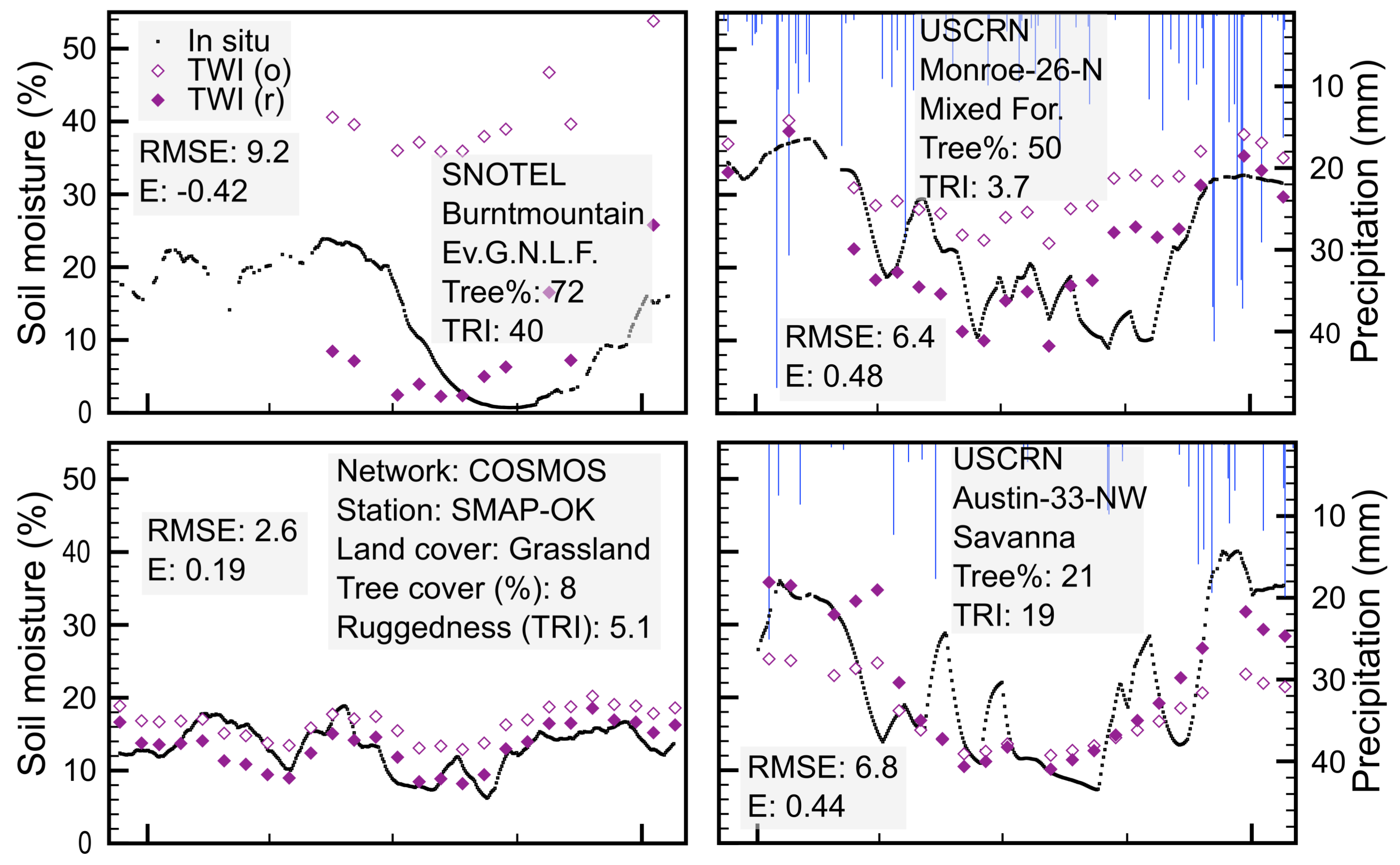
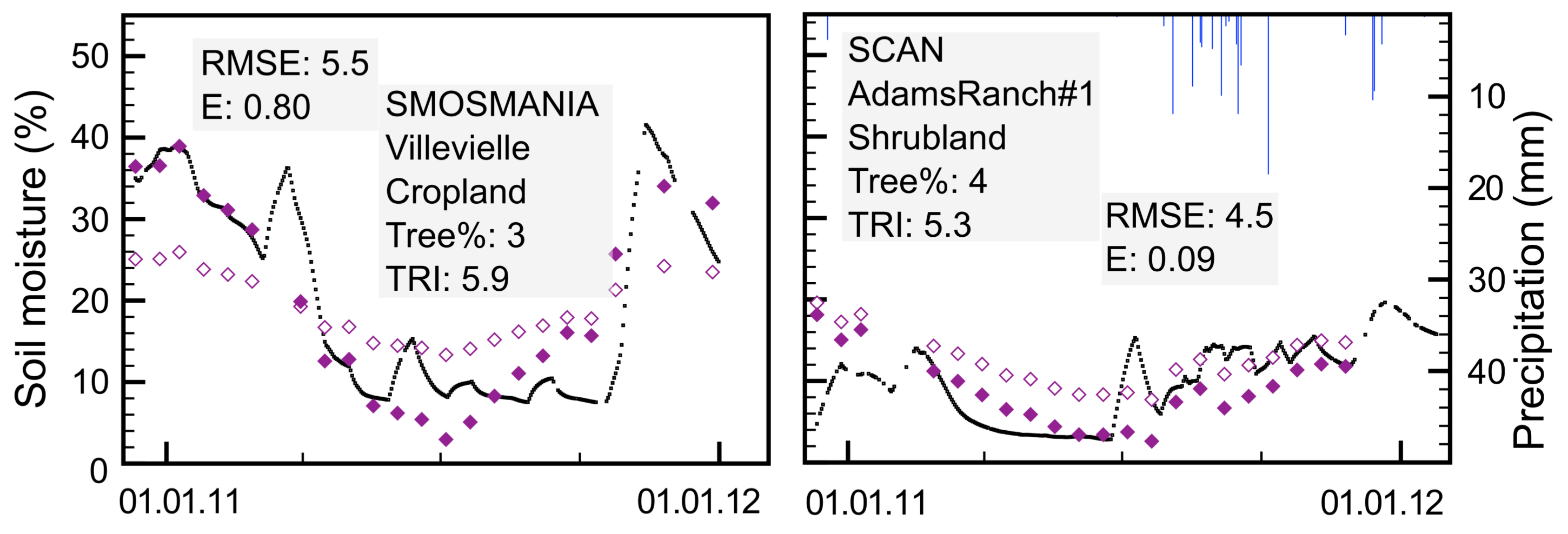
2.3. TWI Performance Validation

Volumetric soil moisture estimates were compared to in situ observed soil wetness retrieved from the International Soil Moisture Network (ISMN). Only the top–most measurements (usually 5 cm) from each ISMN in situ probe were used. Data recordings tagged as erroneous or suspicious were omitted. In situ stations with less than 6 observations coinciding with MODIS TWI estimates were discarded. The data for probes falling within the same MODIS pixel were averaged and from a total of 1040 available in situ time series records for the study period, 823 were used in the validation, representing 745 different MODIS pixels (Table S1).
The actual date of each MODIS TWI estimate is unknown, and was thus set to represent the 8th day of each 16-day interval. For the model validation the diurnal site data were smoothed using a 16-day moving average window. The validation was performed for all probes (global) and by dividing the Earth into three regions, the tropics (between 23° latitudes), the sub-tropics (23° to 46° latitude) and the temperate zone (46° to 70° latitude).
Two different aggregation techniques were used in the validation: (i) direct assembly and; (ii) assembly after local (per in situ station) assimilation. The direct assembly simply aggregates all pairs of modeled and in situ data. Local assimilation rescales the mean ( Θ ¯ ) and variance ( σ 2 ) of the MODIS TWI estimated soil moisture to fit those of the in situ data (only using matching data pairs) thus removing any bias:
Θ m = ( Θ r Θ ¯ T W I ) σ ( Θ i ) σ ( Θ T W I ) + Θ ¯ i
where Θ m is the soil moisture model after assimilation and Θ i the in situ observed soil moisture. Statistical performance was validated using the coefficient of determination, root-mean-square error (RMSE), the Pearson correlation coefficient and model efficiency E:
E = 1 ( Θ o Θ m ) 2 ( Θ o Θ ¯ o ) 2
where Θ ¯ o is the mean of observed soil moisture, and Θ m is modeled and Θ o observed soil moisture for matching data pairs.

2.4. TWI Compared to Microwave Soil-Moisture Products

To compare MODIS TWI (expressed as ΘTWI) to the standard level 3 (L3) soil moisture products from SMOS and AMSR-E, TWI was resampled to a coarser spatial scale averaging the original resolution data. To avoid influences from e.g., water bodies, the re-scaling was set to 13 km rather than 25 km (the spatial scales of the SMOS and AMSR-E L3 products). The routine soil moisture retrieval algorithms for SMOS and AMSR-E discard dubious observations including recordings disturbed by RFI and from densely vegetated landscapes. In order to reduce artificial biases in the comparison of the performances of the three sensors and their respective models, only in situ recordings closely matching SMOS observations (+/− 1 day) were used. With a revisit period of 2 to 3 days all sites and periods with SMOS observations are included for the validation of AMSR-E and MODIS TWI, whereas in situ stations lacking matching SMOS observations, as well as longer periods lacking SMOS observations in other stations, were not used. For the year 2011, 683 stations (723 individual probes) with data coinciding with regions with soil moisture observations by the SMOS sensor were available from ISMN. The data for all probes falling within the same image pixel (at 500 m, 13 km and 25 km spatial resolutions respectively) were averaged and only sites with at least 6 coinciding observations from the ground data and the respective sensor were used in the validation.

2.5. Trend Detection

The MCD43A4 product lacks observations during seasons with constant cloud cover, particularly cumbersome over forested tropical regions. To fill in missing observations the overall seasonal TWI cycle for the whole study period (2001–2016) was first extracted for each cell. For cells with missing observations, a weighted linear interpolation assigns exponentially declining weights to adjacent dates with valid observations. The missing value is then estimated by a linear interpolation of the nearest dates with valid observations, and adjusted for the overall seasonal value.
For the trend detection, the TWI data were aggregated to annual average values and the monotonic trend calculated from the annual averages. The trends were calculated for the whole period 2001 to 2016 disregarding any change points. Trend significance is determined from the MK test, with the strength of the trend estimated from the median slope of Theil-Sen regressions.

3. Results

3.1. Model Performance

Globally TWI correctly captures the soil moisture variations (increases and decreases) for three out of four in situ stations (Table 3). For the tropical and sub–tropical regions, the TWI time–series variations are significantly correlated to approximately 40% of the ground stations, decreasing to 30% for temperate region stations.
Globally MODIS TWI has an aggregated bias of 2.5, an RMSE of 14.0 and a model efficiency of −0.56 compared to the in situ data (Table 4). The soil moisture variation estimated by MODIS TWI, expressed as the standard deviation ( σ ), is lower than the σ of the global in situ data (9.6 compared to 11.2 ), with the difference being significant (Levene’s test <0.05).
The regionalized results show that TWI has a negative bias for the tropics (−3.0) and a higher bias for the temperate zone (8.0). The temperate zone TWI estimates also have a much larger σ , and an RMSE that is significantly larger than for any other region (p < 0.05). The unbiased results show lower RMSE for the cosmic–ray probes and for the tropical region. The global variations in model performance are explored in Figure 3 (corresponding statistical results are reported in Table S1). Figure 4 illustrates the TWI results for ISMN stations representing different regions, land cover and tree cover.

3.2. Comparison with Microwave Soil Moisture Products

Table 5 compares the performance of soil moisture models from the MODIS (TWI), AMSR-E and SMOS sensors. All models have significant biases (p < 0.05), with the MODIS TWI models having a smaller positive bias and AMSR-E and SMOS larger negative biases. All global models fail to capture the dynamic range in soil moisture as observed by the in situ data (Levene’s p-test < 0.05). SMOS has the highest correlation with the in situ data ( r 2 = 0.24), but the large bias causes the global efficiency (E) to be low. With the soil moisture estimates unbiased, SMOS has a significantly lower RMSE compared to AMSR-E and TWI, and AMSR-E has a significantly lower RMSE compared to TWI. The regionalized data (Table S2) shows that the global MODIS TWI models have a pronounced trend in both r 2 and model efficiency E, with better results for the tropical region, declining at higher latitudes. Figures S1 and S2 compare the performances of TWI, AMSR-E and SMOS for stations representing different ISMN networks and land cover.

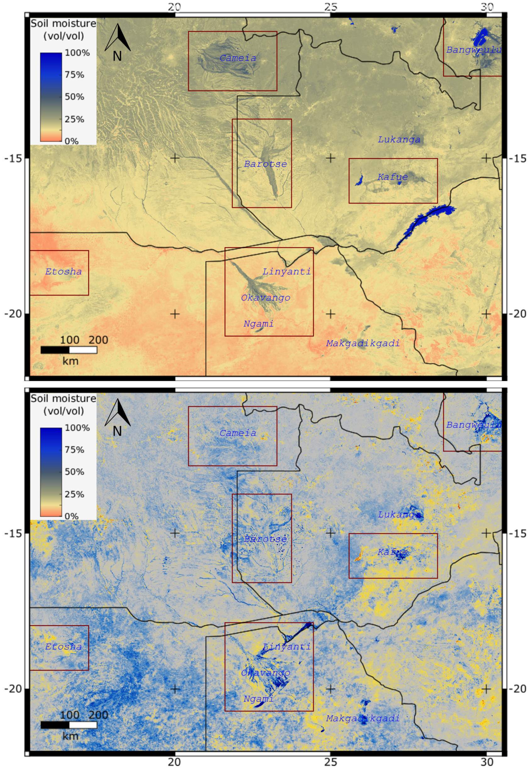
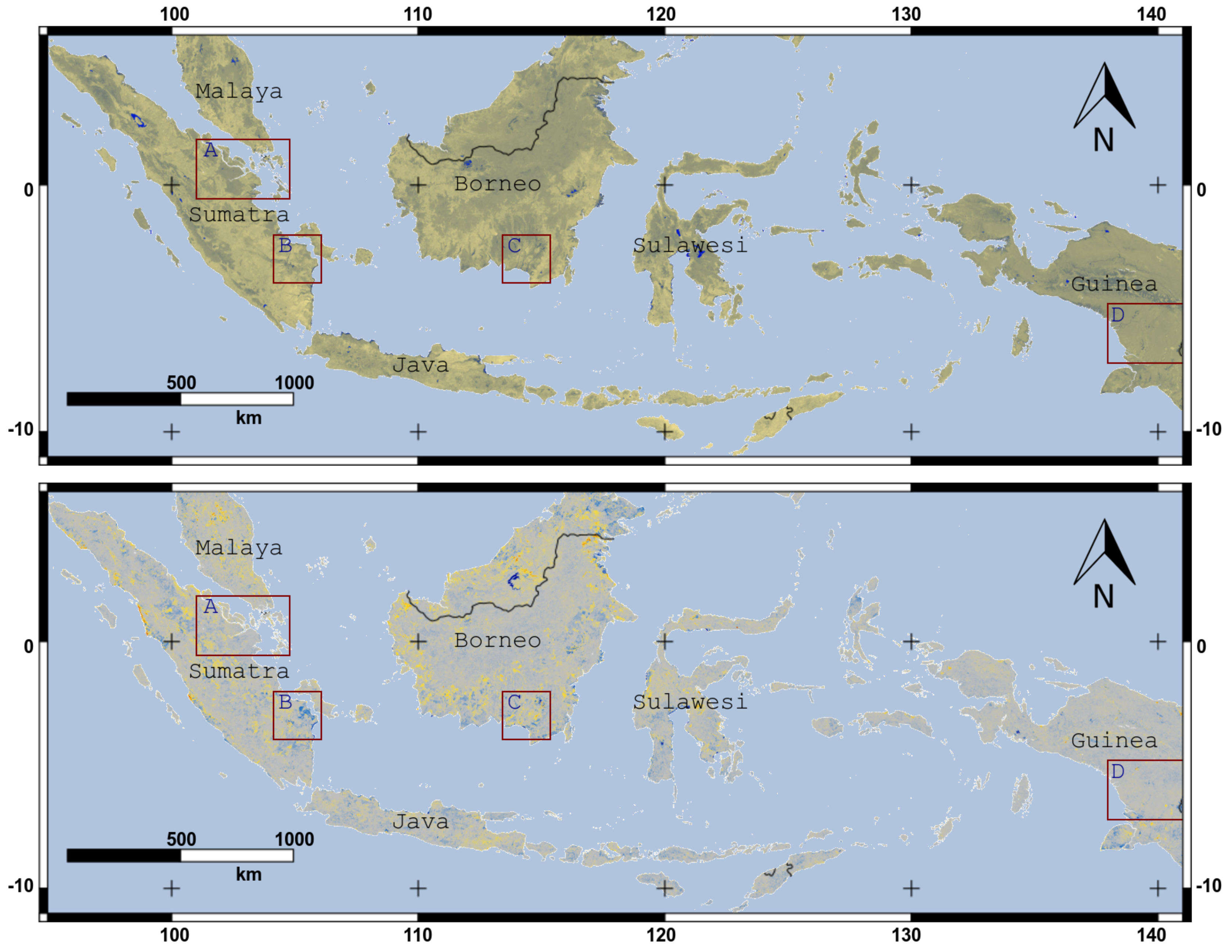
3.3. Soil Moisture Trends

Applying TWI for detecting decadal changes in soil moisture are illustrated in Figure 5, Figure 6 and Figure 7. Maps showing the minimum and maximum wetness for each study region are included in the Supplement (Figure S3: Southern Africa; Figure S10: South East Asia; Figure S15: Western Amazon). The supplement also includes larger scale maps of the wetlands/peatlands indicated in Figure 5, Figure 6 and Figure 7, including maps over areas that have experienced significant monotonic trends in soil moisture over the period 2001 to 2016, and excerpts of the wetland/peatland map presented in [18].

4. Discussion

In this study it has been assumed that the in situ station data are accurate, both regarding the soil moisture conditions and in geographical positions, and that the recorded soil moisture represent the footprint of a MODIS pixel. The positional errors are, however larger than the side of a MODIS pixel for some stations, and only stations equipped with cosmic-ray probes capture the soil moisture over an area approximately equaling the area covered by a MODIS pixel. Further, the exact date of each pixel in the MODIS MCD43A4 product is unknown, and the temporal difference between TWI and the ground measured soil moisture can differ by up to 8 days.

4.1. Model Performance

The performance of TWI varies both between regions and individual stations within the regions. The temporal soil moisture variations are captured with significant correlation for approximately 4 out of 10 ground stations. For a quarter of the ground stations, TWI fails to capture the soil moisture dynamics. Possible explanations for the inaccuracies include: vegetation phenology perturbing the TWI estimations through e.g., leaf water content and ground shadows, and non-linear reflectance responses at different soil moisture levels for different soil minerals.
TWI soil moisture estimates are biased related to site specific conditions, in particular related to vegetation cover and soil properties (Table S1). Inaccuracies related to soil and bedrock conditions include: underestimation in regions with light soil (e.g., quarts dominated arenosois), and over-estimated in regions with darker surfaces (e.g., vertisols, andosols and basaltic outcrops). Dense vegetation stands also perturb TWI: dense stands of e.g., papyrus and reed lead to under-estimations whereas dense moist forests and dark (needleleaf) forests leads to over–estimation. The over–estimations in forested locations are most likely related to shadowed soil surfaces and leaf water content.
The Gram-Schmidt orthogonalization applied for spectral unmixing and retrieval of the linearly transformed vectors representing different biophysical materials is less stable compared to other orthogonalization algorithms. However, as the TWI definition only requires up to the fourth orthogonalized vector, this is of no concern in this study. The primary problem with the conceptual LMM approach is that the same spectral endmembers (eigen–values) are applied for the global region rather than being adjusted to local conditions. The varying spectral properties of different (soil) minerals distort the TWI—illustrated by the theoretical values for dark and light soil, and water saturated dark and light soil in Figure 1. Variations in vegetation reflection, both regarding vegetation types and leaf water status are also disregarded. Ground shadows cause problems both in forests (in particular needleleaf forests) and in topographic complex terrain. The latter could potentially be solved by applying terrain correction to the image data as a preparatory step. Adjusting TWI for vegetation phenology and leaf water status could possibly be done using the image data itself but would probably benefit from incorporating a vegetation growth model.
The unbiased model results with a global RMSE of 8.5 (v/v expressed as percentage), reduced to 5.3 for cosmic-ray probes are comparable to the results obtained from microwave BT data [42,46], with single stations comparing well with stations reported in these studies (cf. Table S1 and corresponding tables in Draper et al. [46], and Jackson et al. [42]).

4.2. Comparison with Microwave Soil Moisture Products

The global comparison of TWI with AMSR-E and SMOS soil moisture products (Table 5) does not indicate that any sensor performs universally better than the others. The unbiased results show that SMOS has a significantly lower RMSE compared to the other sensors after assimilation. SMOS also has a more stable performance across the three latitudinal regions used in this study (Table S2).
From several aspects, both optical and microwave image data are hampered by related problems when adapted for mapping soil moisture. Vegetation and leaf water contents are not completely suppressed. Edaphic conditions relating both to soil mineral compositions, organic matter content, porosity and texture offsets the derived moisture signals for optical data and also perturb the microwave data. Soil moisture estimates from microwave data in general rely on radiative transfer models or machine learning [79,80], either using only the microwave data (e.g., [81]), but more commonly supported with ancillary datasets adjusting for the effects of surface roughness, vegetation and the occurrence of e.g., wetlands and open water. The TWI algorithm presented in this study is one of only few examples in developing algorithms for directly retrieving soil moisture estimates from optical images and was developed without any ancillary data.

4.3. Soil Moisture Trends

The biases reported above are of less concern when applying TWI for trend studies, except when vegetation conditions changes during the study period (e.g., through deforestation). The mis–representation of soil moisture dynamics is of a larger concern. Assuming that vegetation growth varies from year to year dependent on water availability, changes in leaf water status and ground shadows would theoretically reinforce any detected trends. I thus suspect that the presented maps of change are more likely to over–estimate than under–estimate changes in forested regions.
Areas with well known changes in moisture conditions over the past decades, including Lake Ngami and the Makgadikgadi pans in Botswana (Figure 5 and Figure S7) are captured as expected. In Indonesia the site of the Mega Rice project in Kalimantan (Borneo, site C, Figure 6 and Figure S13) shows relatively large variations in both absolute wetness and in monotonic trends. Whether the drying in the Brazilian Amazon (along the Bolivian border) (Figure 7 and Figure S18) is a true drying or an effect of deforestation is not explored.
As I have not been able to identify any soil moisture time–series data representing wetlands or peatlands, it has not been possible to validate the results of the change detection quantitatively. Before such a validation can be undertaken, the usefulness of the change detection is primarily as a monitoring tool for identifying threatened peatlands and wetlands. The wetland/peatland map against which the monotonic trends in soil moisture are compared (see Supplement) represent the year 2011 and the comparison was thus restricted to graphical.
The lack of openly accessible data on ground water tables and soil moisture content for wetlands and peatlands in the global pantropical region is remarkable. The huge carbon storage and the anthropogenic and climate pressure on wetlands and peatlands can potentially lead to the release of large amounts of carbon dioxide.

4.4. Further Development

In this study TWI was compared to the top–soil moisture content. The study suggests that leaf–water status and vegetation shadows influences the TWI with deeper shadows and higher content of soil–water elevating TWI. If these suggestions carries validity, TWI could be adjusted regarding vegetation and leaf–water status and tested as a predictor for moisture content in the deeper soil–column.
In laboratory studies, estimates of soil moisture have been improved by adjusting for inherent mineral brightness. A similar adjustment could be applied to TWI either by using ancillary data on the regolith composition or by using reference wetness data. As the available in situ data is scarce, and the station data usually lack descriptions on mineral compositions, an alternative would be to downscale microwave derived soil moisture products (e.g., from SMAP) using TWI itself and then assign a pixel-wise adjustment factor.

5. Conclusions

The developed algorithm, the Transformed Wetness Index (TWI), suffers from biases caused by mineral compositions and vegetation and most likely also from shadows and leaf water content. The estimated temporal variations in soil moisture are probably also affected by vegetation phenology and non-linear responses in soil-reflectance related to soil moisture. The biases could potentially be reduced by local adjustments, whereas the failures in estimating variations would require additional data from e.g., vegetation growth models or microwave sensors.
TWI bypasses some of the drawbacks that hamper determination of soil surface wetness from optical data; atmospheric attenuations including cloud contaminations are negligible, MODIS includes three SWIR bands, and the vegetation signal influence is reduced through a pixel unmixing orthogonalization and omitting vegetation in a subsequent non-linear normalized differencing. When compared to in situ probed soil moisture the TWI global RMSE was estimated at 14.0 (v/v expressed as percentage) compared to 745 ground observation sites (11.6 when compared to non forested sites). The RMSE is reduced to 8.5 (8.0 for non forests) for unbiased data. MODIS TWI performs better compared to cosmic-ray probes (unbiased RMSE equal to 5.3) with a footprint equalling the spatial resolution of MODIS data. TWI is outperformed by microwave BT data but has a much higher spatial resolution. Consequently TWI might be an alternative for downscaling of microwave derived soil moisture products.
TWI should be regarded as a complement to microwave soil moisture estimates useful for (1) filling in historical trends; (2) estimating soil moisture dynamics at higher spatial resolution; and (3) potentially downscaling absolute soil moisture estimates. Applied to multi–year time–series TWI can be used as a screening tool for changes in soil moisture conditions and for identifying potential hot spots (cool spots) of wetland/peatland degradation (growth).

Supplementary Materials

The following are available online at https://www.mdpi.com/2072-4292/10/4/611/s1, Figure S1: Comparison of in situ and satellite derived soil moisture estimates from SMOS, AMSR-E and the MODIS Transformed Wetness Index (TWI), Figure S2: Same time-series and sensors as in Figure S1 but with each soil moisture product unbiased to the in situ stations, Figure S3: Estimated minimum and maximum soil moisture content for parts of Southern Africa for the period 2001-2016, Figure S4: Etosha pans in Namibia, Figure S5: Cameia wetlands in Angola, Figure S6: Barotse floodplains in Zambia, Figure S7: Okavango and Linyanti swamps and Lake Ngmai in Botswana, Figure S8: Kafue flats in Zambia, Figure S9: Bangweulu Lake and wetlands in Zambia, Figure S10: Estimated minimum and maximum soil moisture content for Indonesia for the period 2001-2016, Figure S11: Central Sumatra (A), Figure S12: South East Sumatra (B), Figure S13: Southern Borneo (C, the mega rice project, Kalimantan), Figure S14: South Western Guinea (D), Figure S15: Estimated minimum and maximum soil moisture content for the Western Amazon basin for the period 2001-2016, Figure S16: Pastanza-Marañon (Peru), Figure S17: South central Amazon (Brazil), Figure S18: South Western Amazon basin (across the Bolivian-Brasilian border), Table S1: Statistics of fit between soil moisture estimates derived from the MODIS Transformed Wetness Index (TWI) and global in situ stations for the period 2010-12-03 to 2012-02-02, Table S2: Statistics of fit between regionalized soil moisture estimates derived from MODIS TWI, AMSR-E and SMOS, compared to global in situ probes for the period 2010-12-02 to 2012-02-01.

Acknowledgments

The MODIS satellite image data for this paper are available at NASA’s Land Processes Distributed Active Archive Center (LP DAAC). Dataset name: MCD43A3.005. Also the land cover data are available at LP DAAC: Dataset names: MCD12Q1.051. AMSR-E daily level 3 (L3) version 2 (maturity V07-Stage 1) data were downloaded from http://nsidc.org. Daily SMOS L3 data were obtained from the Centre Aval de Traitement des Données SMOS (CATDS), operated for the Centre National d’Etudes Spatiales (CNES, France) by IFREMER (Brest, France). The in situ soil moisture data are available at the International Soil Moisture Network (ISMN) hosted by Vienna University of Technology. The article has benefitted greatly from the comments (and patience) of three anonymous reviewers. The study was partly done in cooperation with the Center for International Forestry Research (CIFOR), with original support from the U.S. Agency for International Development (USAID) Grant #MTO069018.

Conflicts of Interest

The author declares no conflict of interest. The founding sponsors had no role in the design of the study; in the collection, analyses, or interpretation of data; in the writing of the manuscript, and in the decision to publish the results.

References

  1. He, L.; Chen, J.M.; Liu, J.; Bélair, S.; Luo, X. Assessment of SMAP soil moisture for global simulation of gross primary production. J. Geophys. Res. Biogeosci. 2017, 122, 1549–1563. [Google Scholar] [CrossRef]
  2. Prigent, C.; Matthews, E.; Aires, F.; Rossow, W.B. Remote sensing of global wetland dynamics with multiple satellite data sets. Geophys. Res. Lett. 2001, 28, 4631–4634. [Google Scholar] [CrossRef]
  3. Papa, F.; Prigent, C.; Aires, F.; Jimenez, C.; Rossow, W.B.; Matthews, E. Interannual variability of surface water extent at the global scale, 1993–2004. J. Geophys. Res. 2010, 115, D12111. [Google Scholar] [CrossRef]
  4. Rodell, M. Satellite Gravimetry Applied to Drought Monitoring. In Remote Sensing of Drought; Wardlow, B.D., Anderson, M.C., Verdin, J.P., Eds.; CRC Press, Taylor & Francis: Boca Raton, FL, USA, 2012; Chapter 11; pp. 261–277. [Google Scholar]
  5. Moran, S.M.; Peters-Lidard, C.D.; Watts, J.M.; McElroy, S. Estimating soil moisture at the watershed scale with satellite-based radar and land surface models. Can. J. Remote Sens. 2004, 30, 805–826. [Google Scholar] [CrossRef]
  6. Wagner, W.; Blöschl, G.; Pampaloni, P.; Calvet, J.C.; Bizzarri, B.; Wigneron, J.P.; Kerr, Y. Operational readiness of microwave remote sensing of soil moisture for hydrologic applications. Nord. Hydrol. 2007, 38, 1. [Google Scholar] [CrossRef]
  7. Nghiem, S.V.; Wardlow, B.D.; Allured, D.; Svoboda, M.D.; LeComte, D.; Rosencrans, M.; Chan, S.K.; Neumann, G. Microwave Remote Sensing of Soil Moisture, Science and applications. In Remote Sensing of Drought; Wardlow, B.D., Anderson, M.C., Verdin, J.P., Eds.; CRC Press; Taylor & Franciss: Boca Raton, FL, USA, 2012; Chapter 9; pp. 197–226. [Google Scholar]
  8. He, L.; Chen, J.M.; Chen, K.S. Simulation and SMAP Observation of Sun-Glint Over the Land Surface at the L-Band. IEEE Trans. Geosci. Remote Sens. 2017, 55, 2589–2604. [Google Scholar] [CrossRef]
  9. Kerr, Y.; Waldteufel, P.; Wigneron, J.P.; Martinuzzi, J.; Font, J.; Berger, M. Soil moisture retrieval from space: The Soil Moisture and Ocean Salinity (SMOS) mission. IEEE Trans. Geosci. Remote Sens. 2001, 39, 1729–1735. [Google Scholar] [CrossRef]
  10. Kerr, Y.H.; Waldteufel, P.; Wigneron, J.P.; Delwart, S.; Cabot, F.; Boutin, J.; Escorihuela, M.J.; Font, J.; Reul, N.; Gruhier, C.; et al. The SMOS Mission: New Tool for Monitoring Key Elements of the Global Water Cycle. Proc. IEEE 2010, 98, 666–687. [Google Scholar] [CrossRef] [Green Version]
  11. Njoku, E.; Jackson, T.; Lakshmi, V.; Chan, T.; Nghiem, S. Soil moisture retrieval from AMSR-E. IEEE Trans. Geosci. Remote Sens. 2003, 41, 215–229. [Google Scholar] [CrossRef]
  12. Merzouki, A.; McNairn, H.; Pacheco, A. Mapping Soil Moisture Using RADARSAT-2 Data and Local Autocorrelation Statistics. IEEE J. Sel. Top. Appl. Earth Obs. Remote Sens. 2011, 4, 128–137. [Google Scholar] [CrossRef]
  13. Chan, S.; Bindlish, R.; O’Neill, P.; Jackson, T.; Njoku, E.; Dunbar, S.; Chaubell, J.; Piepmeier, J.; Yueh, S.; Entekhabi, D.; et al. Development and assessment of the SMAP enhanced passive soil moisture product. Remote Sens. Environ. 2018, 204, 931–941. [Google Scholar] [CrossRef]
  14. Cui, C.; Xu, J.; Zeng, J.; Chen, K.S.; Bai, X.; Lu, H.; Chen, Q.; Zhao, T. Soil Moisture Mapping from Satellites: An Intercomparison of SMAP, SMOS, FY3B, AMSR2, and ESA CCI over Two Dense Network Regions at Different Spatial Scales. Remote Sens. 2017, 10, 33. [Google Scholar] [CrossRef]
  15. Gallant, A. The Challenges of Remote Monitoring of Wetlands. Remote Sens. 2015, 7, 10938–10950. [Google Scholar] [CrossRef]
  16. Lang, M.; Bourgeau-Chavez, L.; Tiner, R.; Klemas, V. Advances in remotely sensed data and techniques for wetland mapping and monitoring. In Remote Sensing of Wetlands: Applications And Advances; Tiner, R., Lang, M., Klemas, V., Eds.; CRC Press: Boca Raton, FL, USA, 2015; Chapter 5; pp. 79–117. [Google Scholar]
  17. Gumbricht, T. Hybrid Mapping of Pantropical Wetlands from Optical Satellite Images, Hydrology, and Geomorphology. In Remote Sensing of Wetlands: Applications and Advances; Tiner, R.W., Lang, M.W., Klemas, V.V., Eds.; CRC Press: Boca Raton, FL, USA, 2015; Chapter 20; pp. 433–452. [Google Scholar]
  18. Gumbricht, T.; Roman-Cuesta, R.M.; Verchot, L.; Herold, M.; Wittmann, F.; Householder, E.; Herold, N.; Murdiyarso, D. An expert system model for mapping tropical wetlands and peatlands reveals South America as the largest contributor. Glob. Chang. Biol. 2017, 23, 3581–3599. [Google Scholar] [CrossRef] [PubMed]
  19. Ordoyne, C.; Friedl, M.A. Using MODIS data to characterize seasonal inundation patterns in the Florida Everglades. Remote Sens. Environ. 2008, 112, 4107–4119. [Google Scholar] [CrossRef]
  20. Landmann, T.; Schramm, M.; Colditz, R.R.; Dietz, A.; Dech, S. Wide Area Wetland Mapping in Semi-Arid Africa Using 250-Meter MODIS Metrics and Topographic Variables. Remote Sens. 2010, 2, 1751–1766. [Google Scholar] [CrossRef]
  21. Aires, F.; Papa, F.; Prigent, C.; Crétaux, J.F.; Berge-Nguyen, M. Characterization and space/time downscaling of the inundation extent over the Inner Niger Delta using GIEMS and MODIS data. J. Hydrometeorol. 2013, 15, 171–192. [Google Scholar] [CrossRef]
  22. Aires, F.; Prigent, C.; Papa, F. Downscaling of inundation extents. In Proceedings of the EGU General Assembly, Vienna, Austria, 27 April–2 May 2014; Volume 16, p. 11668. [Google Scholar]
  23. Aires, F.; Miolane, L.; Prigent, C.; Pham, B.; Fluet-Chouinard, E.; Lehner, B.; Papa, F. A Global Dynamic Long-Term Inundation Extent Dataset at High Spatial Resolution Derived through Downscaling of Satellite Observations. J. Hydrometeorol. 2017, 18, 1305–1325. [Google Scholar] [CrossRef]
  24. Merlin, O.; Al Bitar, A.; Walker, J.P.; Kerr, Y. An improved algorithm for disaggregating microwave-derived soil moisture based on red, near-infrared and thermal-infrared data. Remote Sens. Environ. 2010, 114, 2305–2316. [Google Scholar] [CrossRef] [Green Version]
  25. Merlin, O.; Rudiger, C.; Al Bitar, A.; Richaume, P.; Walker, J.P.; Kerr, Y.H. Disaggregation of SMOS Soil Moisture in Southeastern Australia. IEEE Trans. Geosci. Remote Sens. 2012, 50, 1556–1571. [Google Scholar] [CrossRef] [Green Version]
  26. Piles, M.; Camps, A.; Vall-llossera, M.; Corbella, I.; Panciera, R.; Rüdiger, C.; Kerr, Y.H.; Walker, J. Downscaling SMOS-Derived Soil Moisture Using MODIS Visible/Infrared Data. IEEE Trans. Geosci. Remote Sens. 2011, 49, 3156–3166. [Google Scholar] [CrossRef]
  27. Gillies, R.R.; Carlson, T.N. Thermal Remote Sensing of Surface Soil Water Content with Partial Vegetation Cover for Incorporation into Climate Models. J. Appl. Meteorol. 1995, 34, 745–756. [Google Scholar] [CrossRef]
  28. Petropoulos, G.; Carlson, T.; Wooster, M.; Islam, S. A review of Ts/VI remote sensing based methods for the retrieval of land surface energy fluxes and soil surface moisture. Prog. Phys. Geogr. 2009, 33, 224–250. [Google Scholar] [CrossRef]
  29. Yang, Y.; Guan, H.; Long, D.; Liu, B.; Qin, G.; Qin, J.; Batelaan, O. Estimation of Surface Soil Moisture from Thermal Infrared Remote Sensing Using an Improved Trapezoid Method. Remote Sens. 2015, 7, 8250–8270. [Google Scholar] [CrossRef]
  30. Gumbricht, T. Soil Moisture Dynamics Estimated from MODIS Time Series Images. In Multitemporal Remote Sensing: Methods and Applications; Ban, Y., Ed.; Springer: Berlin, Germany, 2016; pp. 233–253. [Google Scholar]
  31. Muller, E.; Décamps, H. Modeling soil moisture-reflectance. Remote Sens. Environ. 2000, 76, 173–180. [Google Scholar] [CrossRef]
  32. Lobell, D.B.; Asner, G.P. Moisture Effects on Soil Reflectance. Soil Sci. Soc. Am. J. 2002, 66, 722–727. [Google Scholar] [CrossRef]
  33. Kaleita, A.L.; Tian, L.F.; Hirschi, M.C. Relationship Between Soil Moisture Content and Soil Surface Reflectance. Trans. ASAE 2005, 48, 1979–1986. [Google Scholar] [CrossRef]
  34. Gao, Z.; Xu, X.; Wang, J.; Yang, H.; Huang, W.; Feng, H. A method of estimating soil moisture based on the linear decomposition of mixture pixels. Math. Comput. Model. 2013, 58, 606–613. [Google Scholar] [CrossRef]
  35. Zhang, D.; Zhou, G. Estimation of Soil Moisture from Optical and Thermal Remote Sensing: A Review. Sensors 2016, 16, 1308. [Google Scholar] [CrossRef] [PubMed]
  36. Anne, N.J.; Abd-Elrahman, A.H.; Lewis, D.B.; Hewitt, N.A. Modeling soil parameters using hyperspectral image reflectance in subtropical coastal wetlands. Int. J. Appl. Earth Obs. Geoinf. 2014, 33, 47–56. [Google Scholar] [CrossRef]
  37. Ji, L.; Zhang, L.; Wylie, B. Analysis of Dynamic Thresholds for the Normalized Difference Water Index. Photogramm. Eng. Remote Sens. 2009, 75, 1307–1317. [Google Scholar] [CrossRef]
  38. Gao, B.C. NDWI—A normalized difference water index for remote sensing of vegetation liquid water from space. Remote Sens. Environ. 1996, 58, 257–266. [Google Scholar] [CrossRef]
  39. Ceccato, P.; Gobron, N.; Flasse, S.; Pinty, B.; Tarantola, S. Designing a spectral index to estimate vegetation water content from remote sensing data: Part 1: Theoretical approach. Remote Sens. Environ. 2002, 82, 188–197. [Google Scholar] [CrossRef]
  40. Ceccato, P.; Flasse, S.; Grégoire, J.M. Designing a spectral index to estimate vegetation water content from remote sensing data: Part 2 Validation and application. Remote Sens. Environ. 2002, 82, 198–207. [Google Scholar] [CrossRef]
  41. Weidong, L.; Baret, F.; Xingfa, G.; Qingxi, T.; Lanfen, Z.; Bing, Z. Relating soil surface moisture to reflectance. Remote Sens. Environ. 2002, 81, 238–246. [Google Scholar] [CrossRef]
  42. Jackson, T.J.; Cosh, M.H.; Bindlish, R.; Starks, P.J.; Bosch, D.D.; Seyfried, M.; Goodrich, D.C.; Moran, M.S.; Du, J. Validation of Advanced Microwave Scanning Radiometer Soil Moisture Products. IEEE Trans. Geosci. Remote Sens. 2010, 48, 4256–4272. [Google Scholar] [CrossRef]
  43. Reichle, R.H.; Koster, R.D. Bias reduction in short records of satellite soil moisture. Geophys. Res. Lett. 2004, 31, L19501. [Google Scholar] [CrossRef]
  44. Reichle, R.H.; Koster, R.D.; Liu, P.; Mahanama, S.P.P.; Njoku, E.G.; Owe, M. Comparison and assimilation of global soil moisture retrievals from the Advanced Microwave Scanning Radiometer for the Earth Observing System (AMSR-E) and the Scanning Multichannel Microwave Radiometer (SMMR). J. Geophys. Res. Atmos. 2007, 112, D09108. [Google Scholar] [CrossRef]
  45. Wagner, W.; Naeimi, V.; Scipal, K.; Jeu, R.; Martínez-Fernández, J. Soil moisture from operational meteorological satellites. Hydrogeol. J. 2007, 15, 121–131. [Google Scholar] [CrossRef]
  46. Draper, C.S.; Walker, J.P.; Steinle, P.J.; de Jeu, R.A.M.; Holmes, T.R.H. An evaluation of AMSR–E derived soil moisture over Australia. Remote Sens. Environ. 2009, 113, 703–710. [Google Scholar] [CrossRef]
  47. Dall’Amico, J.T.; Schlenz, F.; Loew, A.; Mauser, W. First Results of SMOS Soil Moisture Validation in the Upper Danube Catchment. IEEE Trans. Geosci. Remote Sens. 2012, 50, 1507–1516. [Google Scholar] [CrossRef]
  48. Draper, C.; Reichle, R.; de Jeu, R.; Naeimi, V.; Parinussa, R.; Wagner, W. Estimating root mean square errors in remotely sensed soil moisture over continental scale domains. Remote Sens. Environ. 2013, 137, 288–298. [Google Scholar] [CrossRef]
  49. Nash, J.E.; Sutcliffe, J.V. River flow forecasting through conceptual models part I—A discussion of principles. J. Hydrol. 1970, 10, 282–290. [Google Scholar] [CrossRef]
  50. Pearson, K. Notes on regression and inheritance in the case of two parents. Proc. R. Soc. Lond. 1895, 58, 240–242. [Google Scholar] [CrossRef]
  51. Zreda, M.; Desilets, D.; Ferré, T.P.A.; Scott, R.L. Measuring soil moisture content non-invasively at intermediate spatial scale using cosmic-ray neutrons. Geophys. Res. Lett. 2008, 35, L21402. [Google Scholar] [CrossRef]
  52. Jha, M.K.; Singh, A.K. Trend analysis of extreme runoff events in major river basins of Peninsular Malaysia. Int. J. Water 2013, 7, 142. [Google Scholar] [CrossRef]
  53. Martinez, C.J.; Maleski, J.J.; Miller, M.F. Trends in precipitation and temperature in Florida, USA. J. Hydrol. 2012, 452-453, 259–281. [Google Scholar] [CrossRef]
  54. Modarres, R.; Sarhadi, A. Rainfall trends analysis of Iran in the last half of the twentieth century. J. Geophys. Res. 2009, 114, D03101. [Google Scholar] [CrossRef]
  55. Sonali, P.; Nagesh Kumar, D. Review of trend detection methods and their application to detect temperature changes in India. J. Hydrol. 2013, 476, 212–227. [Google Scholar] [CrossRef]
  56. Hu, Z.; Zhou, Q.; Chen, X.; Qian, C.; Wang, S.; Li, J. Variations and changes of annual precipitation in Central Asia over the last century. Int. J. Climatol. 2017, 37, 157–170. [Google Scholar] [CrossRef]
  57. Zhao, W.; Du, H.; Wang, L.; He, H.S.; Wu, Z.; Liu, K.; Guo, X.; Yang, Y. A comparison of recent trends in precipitation and temperature over Western and Eastern Eurasia. Q. J. R. Meteorol. Soc. 2018, 144, 604–613. [Google Scholar] [CrossRef]
  58. Sayemuzzaman, M.; Jha, M.K. Seasonal and annual precipitation time series trend analysis in North Carolina, United States. Atmos. Res. 2014, 137, 183–194. [Google Scholar] [CrossRef]
  59. Mann, H.B. Nonparametric Tests Against Trend. Econometrica 1945, 13, 245. [Google Scholar] [CrossRef]
  60. Muhlbauer, A.; Spichtinger, P.; Lohmann, U. Application and Comparison of Robust Linear Regression Methods for Trend Estimation. J. Appl. Meteorol. Climatol. 2009, 48, 1961–1970. [Google Scholar] [CrossRef]
  61. Theil, H. A Rank-Invariant Method of Linear and Polynomial Regression Analysis. Proc. R. Neth. Acad. Sci. 1950, 53, 386–392. [Google Scholar]
  62. Sen, P.K. Estimates of the Regression Coefficient Based on Kendall’s Tau. J. Am. Stat. Assoc. 1968, 63, 1379–1389. [Google Scholar] [CrossRef]
  63. Ochsner, T.E.; Cosh, M.H.; Cuenca, R.H.; Dorigo, W.A.; Draper, C.S.; Hagimoto, Y.; Kerr, Y.H.; Njoku, E.G.; Small, E.E.; Zreda, M. State of the Art in Large-Scale Soil Moisture Monitoring. Soil Sci. Soc. Am. J. 2013, 77, 1888. [Google Scholar] [CrossRef] [Green Version]
  64. Dorigo, W.A.; Wagner, W.; Hohensinn, R.; Hahn, S.; Paulik, C.; Xaver, A.; Gruber, A.; Drusch, M.; Mecklenburg, S.; van Oevelen, P.; et al. The International Soil Moisture Network: A data hosting facility for global in situ soil moisture measurements. Hydrol. Earth Syst. Sci. 2011, 15, 1675–1698. [Google Scholar] [CrossRef]
  65. Danielson, J.; Gesch, D. Global Multi-resolution Terrain Elevation Data 2010 (GMTED2010)—Open-File Report 2011–1073; Technical Report 2011–1073; USGS: Reston, VA, USA, 2011.
  66. Wilson, M.F.J.; O’Connell, B.; Brown, C.; Guinan, J.C.; Grehan, A.J. Multiscale Terrain Analysis of Multibeam Bathymetry Data for Habitat Mapping on the Continental Slope. Mar. Geod. 2007, 30, 3–35. [Google Scholar] [CrossRef]
  67. Hijmans, R.J.; Cameron, S.E.; Parra, J.L.; Jones, P.G.; Jarvis, A. Very high resolution interpolated climate surfaces for global land areas. Int. J. Climatol. 2005, 25, 1965–1978. [Google Scholar] [CrossRef]
  68. Njoku, E. AMSR-E/Aqua Daily L3 Surface Soil Moisture, Interpretive Parameters, & QC EASE-Grids. version 2; AMSR_E_L3_DailyLand_V07. 2004. Available online: http://nsidc.org/data/ae_land3 (accessed on 15 April 2018).
  69. Kauth, R.J.; Thomas, G.S. The Tasseled Cap—A graphic description of the spectral-temporal development of agricultural crops as seen by Landsat. In Proceedings of the Symposium on Machine Processing of Remotely Sensed Data, West Lafayette, Indiana, 29 June–1 July 1976; pp. 4B41–4B51. [Google Scholar]
  70. Crist, E.P.; Cicone, R.C. A physically-based transformation of thematic mapper data—The TM tasseled cap. IEEE Trans. Geosci. Remote Sens. 1984, GE-22, 256–263. [Google Scholar] [CrossRef]
  71. Yarbrough, L.D.; Easson, G.; Kuszmaul, J.S. Quickbird 2 Tasseled Cap Transform Coefficients: A Comparison of Derivation Methods. In Proceedings of the Pecora 16 Global Priorities in Land Remote Sensing, Sioux Falls, SD, USA, 23–27 October 2005. [Google Scholar]
  72. Lobser, S.E.; Cohen, W. MODIS tasselled cap: Land cover characteristics expressed through transformed MODIS data. Int. J. Remote Sens. 2007, 28, 5079–5101. [Google Scholar] [CrossRef]
  73. Small, C.; Milesi, C. Multi-scale standardized spectral mixture models. Remote Sens. Environ. 2013, 136, 442–454. [Google Scholar] [CrossRef]
  74. Baret, F.; Jacquemoud, S.; Hanocq, J.F. The soil line concept in remote sensing. Remote Sens. Rev. 1993, 7, 65–82. [Google Scholar] [CrossRef]
  75. Richardson, A.J.; Wiegand, C.L. Distinguishing vegetation from soil background information. Photogramm. Eng. Remote Sens. 1977, 43, 1541–1552. [Google Scholar]
  76. Fox, G.A.; Sabbagh, G.J.; Searcy, S.W.; Yang, C. An Automated Soil Line Identification Routine for Remotely Sensed Images. Soil Sci. Soc. Am. J. 2004, 68, 1326–1331. [Google Scholar] [CrossRef]
  77. Paris, J.F. FAQs by Jack E: Grand Unified Vegetation Index Images. 2005. Available online: http://www.microimages.com/sml/ParisScripts/FAQsbyJackE.pdf (accessed on 15 April 2018).
  78. Baldridge, A.; Hook, S.; Grove, C.; Rivera, G. The ASTER spectral library version 2.0. Remote Sens. Environ. 2009, 113, 711–715. [Google Scholar] [CrossRef]
  79. Mladenova, I.; Jackson, T.; Njoku, E.; Bindlish, R.; Chan, S.; Cosh, M.; Holmes, T.; de Jeu, R.; Jones, L.; Kimball, J.; et al. Remote monitoring of soil moisture using passive microwave-based techniques—Theoretical basis and overview of selected algorithms for AMSR-E. Remote Sens. Environ. 2014, 144, 197–213. [Google Scholar] [CrossRef]
  80. Ali, I.; Greifeneder, F.; Stamenkovic, J.; Neumann, M.; Notarnicola, C. Review of Machine Learning Approaches for Biomass and Soil Moisture Retrievals from Remote Sensing Data. Remote Sens. 2015, 7, 16398–16421. [Google Scholar] [CrossRef]
  81. Santi, E.; Pettinato, S.; Paloscia, S.; Pampaloni, P.; Macelloni, G.; Brogioni, M. An algorithm for generating soil moisture and snow depth maps from microwave spaceborne radiometers: HydroAlgo. Hydrol. Earth Syst. Sci. 2012, 16, 3659–3676. [Google Scholar] [CrossRef]
Figure 1. Iso-lines of surface wetness as estimated from: left) the Perpendicular Wetness Index (PWI) and right) the Transformed WI (TWI). The axis are the same in both panels, representing the soil line (x) and wetness (y) defined from a linear transformation of MODIS satellite reflectance bands. The reference features in the left panel (PWI) are extracted to represent three phenological situations: end of wet season (most faded), peak dry season (intermediate), and end of dry season (un-faded). The seasonality was determined from the worldclim global dataset [67]. The reference features were used in pairs representing wetter and drier conditions to calibrate the eigen–values (orthogonal matrix) defining the soil line and wetness, and the slope of the wetness line. Time-series data over swamp forests and floodplains (see legend) were used to calibrate the non-linearity of TWI as shown in the right panel. In addition to the reference iso-wetness line (PWI = 0) two more perpendicular wetness lines are also shown (PWI = −1000 and PWI = 1000), with the latter having their starting point where the Parallel Background Index (PBI) equals zero. The annotated dots in the right panel (TWI) represent the theoretical values for; DS: dark soil, LS: light soil, W: water, SDS: saturated dark soil, SLS: saturated light soil, and DMS: dry medium soil (medium = equal mixture of light and dark soil spectral end members).
Remotesensing 10 00611 g001
Figure 2. Scatterplots of the Transformed Wetness Index (TWI) versus in situ observed soil moisture. The left panel shows the original MODIS TWI values on the x-axis and in situ measured soil moisture on the y-axis. The black line shows the adopted model (Equation (9)) for converting MODIS TWI to volumetric soil moisture. The right panel shows MODIS TWI converted to soil moisture (ΘTWI) as indicated in the left panel, and then assimilated to fit the local statistical moments of the measured soil moisture of each in situ station. The color codes reveal the dominating land cover (from MODIS product MCD12Q1) of each sample site.
Remotesensing 10 00611 g002
Figure 3. Scatterplots of the MODIS Transformed Wetness Index (ΘTWI) compared to in situ data. Color codes indicate the dominating land cover (from MODIS product MCD12Q1) of each sample site, and symbol form represents the latitudinal region. The upper left panel shows the relation between the Terrain Ruggedness Index (TRI) (derived from GMTED2010) and the Random Mean Square Error (RMSE); the lower left panel instead shows the relation between tree cover (from MODIS product MOD44B) and RMSE; the upper right panel shows the model bias as a function of tree cover; and the lower right panel shows the tree cover plotted against the difference (bias) in variance ( σ ) between the TWI model and the in situ data.
Remotesensing 10 00611 g003
Figure 4. Comparison of soil moisture observations from in situ station data and soil moisture estimated by the MODIS Transformed Wetness Index (ΘTWI). Each panel shows both the global MODIS TWI model (o) and the unbiased model (r), with the statistical fit shown for the latter. Precipitation data on right and top axis (right column panels only). Legend codes in the two upper left panels (Ev.G.N.L.F. = evergreen needleleaf forest).
Remotesensing 10 00611 g004aRemotesensing 10 00611 g004b
Figure 5. Estimated average (top) and absolute volumetric change in soil moisture for parts of Southern Africa for the period 2001-2016. The wetness is calculated from the MODIS Transformed Wetness Index for the period January 2001 to December 2016. All wetland regions outlined (maroon boundaries) are shown in larger scale maps in the supplement.
Remotesensing 10 00611 g005
Figure 6. Estimated average (top) and absolute volumetric change in soil moisture for Indonesia for the period 2001–2016. The wetness is calculated from the MODIS Transformed Wetness Index for the period January 2001 to December 2016. For legends see Figure 5. All regions outlined (maroon boundaries) are shown in larger scale maps in the supplement.
Remotesensing 10 00611 g006
Figure 7. Estimated average (top) and absolute volumetric change in soil moisture for the Western Amazon basin for the period 2001–2016. The wetness is calculated from the MODIS Transformed Wetness Index for the period January 2001 to December 2016. For legends see Figure 5. All regions outlined (maroon boundaries) are shown in larger scale maps in the supplement.
Remotesensing 10 00611 g007aRemotesensing 10 00611 g007b
Table 1. Reflectance factor value (reflectance ∗ 10 5 ) mean and standard deviation (in parenthesis) for global spectral endmembers identified for tropical MODIS (product MCD43A4) tiles (band order given as they appear in the MCD43A4 product).
MaterialRedNIRBlueGreenSWIRaSWIRbSWIRc
D a r k s o i l 61098551863113101249869
(208)(397)(220)(269)(676)(739)(556)
L i g h t s o i l 127916748091099210222131816
(292)(430)(226)(220)(746)(909)(797)
P V 4934431296790404024211013
(130)(425)(78)(124)(298)(209)(226)
W a t e r 290202386402198200135
(326)(158)(141)(283)(124)(105)(82)
Table 2. Dark soil offset (reflectance ∗ 10 5 ) and orthogonal matrix values (eigen–values) used for defining the TWI reference wetness-line. The wetness line is defined from the soil line and water components, while photosynthetic vegetation (PV) and non-PV are omitted (band order given as in the MCD43A4 product).
MaterialRedNIRBlueGreenSWIRaSWIRbSWIRc
O f f s e t 5631008147507153118361699
S o i l l i n e 0.3148120.3209700.3594560.3363640.2497720.6573340.247078
P V −0.1936660.798701−0.140345−0.0947620.390175−0.199024−0.322562
N o n P V 0.4825200.134057−0.0255350.3476070.071952−0.6538130.441669
W a t e r 0.1881770.0383640.4939170.350060−0.358132−0.173122−0.662112
Table 3. Pearson correlation coefficients for the relation between TWI and in situ soil moisture probes from the ISMN network, expressed as the percentage of stations with positive correlations and significantly positive correlations. Only stations with 12 or more coinciding values are included.
2∗Region/NetworkPearson Corr. > 0
% of n Stations
Pearson Corr. > 0 and p < 0.05
% of n Stations
Stations
n
Global7440459
Tropical804015
Sub-tropical7441417
Temperate622927
COSMOS783132
Table 4. Statistics of fit between volumetric soil moisture estimated from the MODIS Transformed Wetness Index and in situ probes from the International Soil Moisture Network (3 December 2010 to 2 February 2012). Global results represent data without rescaling. Unbiased results have ΘTWI means ( x ¯ ) and standard deviations ( σ ) locally fitted to the in situ data. The difference between the global and unbiased results equals the model bias. Statistical significances for differences in x ¯ and RMSE are calculated using two-tailed student t-test. The significance of differences in variance are calculated using Levene’s test. The correlation coefficients (r2) and model efficiencies (E) for assimilated model results are given for each in situ site in Table S1.
Model x ¯ σ RMSE r 2 En stnn
Global region
G l o b a l 21.9 a9.6 b14.00.02−0.5674512,294
U n b i a s e d 19.411.28.574512,294
Tropical region
G l o b a l 19.0 b,d11.4 b,c13.40.260.1619372
U n b i a s e d 22.0 c14.7 c6.3 d19372
Sub-tropical region
G l o b a l 21.4 a,d8.8 b,d13.5 d0.02−0.4865711,036
U n b i a s e d 19.1 d11.1 d8.5 d65711,036
Temperate region
G l o b a l 29.6 a,c14.1 a,c19.4 c0.0−2.269886
U n b i a s e d 21.6 c10.8 d10.2 c69886
COSMOS network (cosmic-ray probes across all regions)
G l o b a l 24.0 a,c11.0 b14.30.07−0.5052771
U n b i a s e d 20.3 c11.7 c5.3 d52771
non Forested sites across all regions
G l o b a l 18.7 b,d6.8 b,d11.6 d0.05−0.095749679
U n b i a s e d 19.1 d11.18.0 d5749679
a Estimated variable significantly higher (p < 0.05) than in situ data; b Estimated variable significantly lower (p < 0.05) than in situ data; c Variable significantly higher (p < 0.05) than for other regions/probes/land cover; d Variable significantly lower (p < 0.05) than for other regions/probes/land cover.
Table 5. Statistics of fit between soil moisture estimates from TWI at the original (o) MODIS spatial resolution (500 m) and resampled (r) to 13 km, and AMSR-E and SMOS (both at 25 km spatial resolution), compared to global in situ probes for the period 2010-12-02 to 2012-02-01. See Table 4 for explanations.
Sensor x ¯ σ RMSE r 2 En stnn
Globalabc
MODIS (o)19.28.112.20.07−0.135166886
MODIS (r)19.67.611.50.110.04686560
AMSR-E12.83.312.00.15−0.1149756,153
SMOS12.29.012.40.24−0.2151752,457
Unbiased d
MODIS (o)18.811.47.15166886
MODIS (r)18.911.46.84686560
AMSR-E18.511.46.349756,153
SMOS18.911.35.651752,457
a All biases are significant (p < 0.05); b All global variances ( σ ) are significantly lower than the variances of the in situ data (Levene’s test < 0.05); c Global RMSE (p = 0.05): MODIS(r) < all others, AMSRE = MODIS(o), (AMSRE and MODIS(o)) < SMOS; d Unbiased RMSE (p = 0.05): SMOS < all others, AMSRE < both MODIS, MODIS(r) < MODIS(o).

