Abstract
In this study, the potential of multispectral airborne laser scanner (ALS) data to model and predict some forest characteristics was explored. Four complementary characteristics were considered, namely, aboveground biomass per hectare, Gini coefficient of the diameters at breast height, Shannon diversity index of the tree species, and the number of trees per hectare. Multispectral ALS data were acquired with an Optech Titan sensor, which consists of three scanners, called channels, working in three wavelengths (532 nm, 1064 nm, and 1550 nm). Standard ALS data acquired with a Leica ALS70 system were used as a reference. The study area is located in Southern Norway, in a forest composed of Scots pine, Norway spruce, and broadleaf species. ALS metrics were extracted for each plot from both elevation and intensity values of the ALS points acquired with both sensors, and for all three channels of the ALS multispectral sensor. Regression models were constructed using different combinations of metrics. The results showed that all four characteristics can be accurately predicted with both sensors (the best R2 being greater than 0.8), but the models based on the multispectral ALS data provide more accurate results. There were differences regarding the contribution of the three channels of the multispectral ALS. The models based on the data of the 532 nm channel seemed to be the least accurate.
1. Introduction
Airborne laser scanner (ALS) data are recognized as the best remote sensing data to model forest structural characteristics [1,2]. Since the late 1990s when the first studies on the application of ALS data in forestry and ecology appeared in the literature [3,4,5] numerous studies have been carried out using ALS data for a great variety of applications. In forestry, the main use is for the prediction of forest volume or other forest characteristics [6], while in the ecology community many studies are also related to animal habitat assessment [7,8,9]. ALS data are also widely used for the prediction of species diversity indices, like the Shannon and Simpson species diversity indices [10].
Indeed, ALS data provide detailed information on tree heights [4], while information related to the spectral signatures of trees is limited, as only one spectral band is usually available—the most common being 1064 nm. Despite this, some studies have applied this limited spectral information in the form of backscatter intensity of the laser signal for the classification of tree species with at least some degree of success when the number of species is small [11]. Recently, considerable effort has been devoted to develop multi/hyperspectral ALS sensors [12,13,14,15]. These sensors can acquire ALS data using different wavelengths providing intensity information in different bands. This is usually done by employing different laser scanners working at different wavelengths [16], even if systems exist that consist of just a single laser working on a broad spectrum and with wavelength separation conducted at the receiver level [14]. The majority of these sensors are still in the prototype stage or they were developed to be terrestrial laser scanners. At the moment the only airborne multispectral ALS sensor commercially available is the Optech Titan, which consists of three laser scanners, called channels, working at 532 nm, 1064 nm, and 1550 nm. This system allows us to have spectral information in three bands and to have a higher point density as the elevation information is aggregated over returns from all three scanners. This sensor was released in the commercial market in 2015, and data acquired with this system was subject to scientific research shortly after the release. However, published studies are still few in number (e.g., [17,18,19,20,21]), and also for forestry and ecology applications [17,22]. In particular Budei et al. [17], Yu et al. [22], and Axelsson et al. [20] focused on tree species classification. Budei et al. [17] showed that species identification accuracy can be improved by using a three-wavelength ALS compared to single-channel ALS systems, especially when tree species diversity is fairly large (seven classes or more). The authors found that the channel at 1550 nm is the most useful for this task. Yu et al. [22] also focused on tree species classification and their results suggest that the channel at 1064 nm contains more information for separating pine, spruce, and birch, followed by the 1550 nm channel and 532 nm channel. Axelsson et al. [20] showed that metrics extracted from both elevation and intensity of multispectral ALS data improve the classification of boreal tree species by more than 30%.
The overall objective of the current study was to explore the potential of the Optech Titan multispectral ALS data in modelling and predicting forest characteristics at the plot level. The results obtained with the Optech Titan were compared to those resulting from adopting data from a standard ALS sensor, i.e., a Leica ALS70 instrument. We focused on four characteristics, namely aboveground biomass (AGB) per hectare, the Gini coefficient of the diameter at breast height, the Shannon diversity index of the tree species, and the number of trees per hectare. These four characteristics are all relevant and of interest to forestry and/or ecological applications. The aboveground biomass per hectare is widely used in ecological studies related to carbon stored in forests [23,24]. Many studies exist that use ALS data for this purpose. The Gini coefficient of the DBHs is a parameter that is useful in order to characterise forest structure [25]. The Shannon diversity index is widely used to map species diversity of forests. The number of trees per hectare can be very useful in combination with other indices to map forest structure and density.
2. Dataset Description
The study area is located in Hadeland municipality, Southern Norway (Figure 1). The field data were collected in August and September 2015 on ten circular sample plots 1000 m2 in size and two circular sample plots 500 m2 in size. Within each sample plot, tree species, diameter at beast height (DBH), and tree coordinates were recorded for all trees with DBH > 3 cm. A total of 1075 trees were recorded of which 71.1% were Norway spruce, 6.8% were Scots pine, and 22.1% were broadleaf. Aboveground biomass of each tree was calculated using the allometric models of Marklund [26]. Field data were accurately co-registered with ALS data using field-measured trees in order to reduce, at a minimum, any error due to data misalignment.
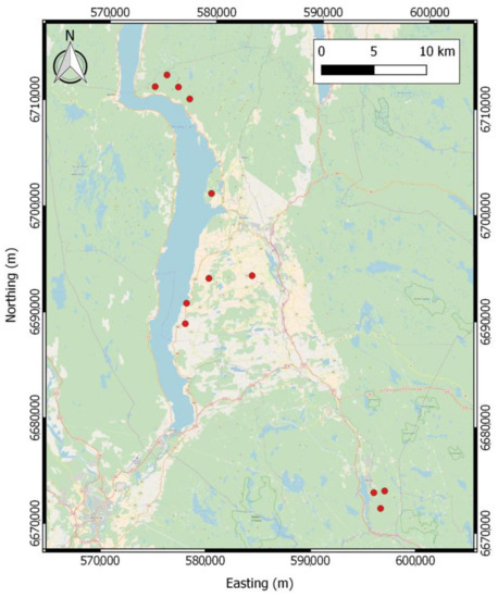
Figure 1.
Location of the 12 field plots (red dots) in Hadeland municipality.
In order to have a higher number of observations for the analysis we split the plots into 44 sub-plots of 250 m2. The original 500 m2 plots were divided along the Y-axis into two crescents, while the 1000 m2 plots were divided along the X and Y axes into four slices. For each sub-plot we computed the aboveground biomass per hectare (AGBha), the Gini coefficient of DBHs (GiniDBHs), the Shannon diversity index (SDI), and the number of trees per hectare (Nha). AGBha per plot was computed as the sum of the AGB of the field-measured trees inside each plot scaled to the hectare level. GiniDBHs was computed as the Gini coefficient of the DBHs of all the field-measured trees inside the plots, SDI was computed as the Shannon diversity index of all the field-measured species inside the plots, and Nha as the number of trees in each plot scaled to the hectare level. Table 1 shows a summary of the field data at the plot level.

Table 1.
Summary of the field data at the plot level.
ALS data were acquired using a Leica ALS70 (Leica Geosystems, St. Gallen, Switzerland) sensor and an Optech Titan (Teledyne Optech, Vaughan, ON, Canada) sensor. The Leica ALS70 data were acquired on 7 September 2014. Up to four returns per pulse were recorded and the resulting density of single and first returns was 10 pts/m2. The Optech Titan data were acquired on 27 April 2016. A summary of the Optech Titan sensor characteristics is presented in Table 2. Up to four returns per pulse were recorded and the resulting density of single and first returns was 38 pts/m2 (14 pts/m2 for channel 1, 21 pts/m2 for channel 2, and 3 pts/m2 for channel 3).
Table 2.
Summary of the Optech Titan sensor characteristics.
3. Methods
3.1. Data Preprocessing
Normalized Z values, i.e., heights above ground, were computed for both datasets by using the lasground tool inside the LAStools (https://rapidlasso.com/lastools/) software. The points with Z values smaller than 0 were removed and so were those greater than 40 m. According to the field data, the largest recorded tree in the plots was 27 m in height and, thus, this operation allowed us to remove any possible outliers from the ALS data.
The intensity value of each ALS point of both sensors was range-calibrated using the following equation:
where is the calibrated intensity, the raw intensity, is the sensor-to-target range, and is the reference range or average flying height. We considered an exponential factor of 2.5 [27] since the environmental factors can be considered stable and the same acquisition parameters and instruments were maintained during the survey [22].
3.2. ALS Metrics Extraction
From each sub-plot, ALS metrics were extracted from both the Leica ALS70 data and the Optech Titan data. The metrics, summarized in Table 3, were extracted for each sub-plot from both the elevation and the intensity of the ALS points using the stdmetrics function of the R package lidR. Additionally, from the Optech Titan data we considered four indices computed by combining the mean sub-plot intensity values () across the three Titan channels:
Table 3.
Metrics extracted from the ALS points.
The ALS metrics were grouped into six sets:
- ALS70: Leica ALS70 metrics;
- TITAN: Optech Titan metrics extracted by considering all points across all channels as a single group of data regardless of the channel;
- TITAN_1_2_3: Optech Titan metrics extracted for each of the channels separately. In this way we extracted each metric three times;
- TITAN_1: Optech Titan metrics extracted only from the first channel of the sensor (1550 nm);
- TITAN_2: Optech Titan metrics extracted only from the second channel of the sensor (1064 nm); and
- TITAN_3: Optech Titan metrics extracted only from the third channel of the sensor (532 nm).
3.3. Exploratory Analyses, Modelling, and Validation
3.3.1. The General Set-Up for the Analyses
The initial 12 plots can be safely considered as independent observations (see the spatial distribution and geographical distances in Figure 1), however, splitting the field plots into two or four sub-plots (see Section 2) introduced a hierarchical structure in the dataset. The lack of independence among the sub-plots has two implications for the statistical analyses: (i) for the ordinary least squares (OLS) regression, which is commonly used for modelling in forest inventory studies, the estimated model coefficients are unbiased, but the variance-covariance estimator of the model coefficients will be biased; and (ii) since the sub-plots are spatially grouped, it is expected that the regression predictions on sub-plots that belong to the same field plot also are correlated, and that would violate the independence assumption when calculating the residual error sum of squares based on the sub-plot level prediction errors (see Section 3.3.5). Moreover, aggregating the sub-plot predictions to the plot level is not meaningful for some of the characteristics, such as the Shannon and the Gini indices, which are scale dependent. Due to this restriction and the scarcity of data, the analyses were performed on the sub-plot level using specific approaches to deal with the nested structure of the dataset.
We started the analyses by exploring the information carried by the Optech Titan intensity data (Section 3.3.2), in order to see whether or not these auxiliary data should be considered as candidate predictors for the forest characteristics. Next, the sets of ALS metrics for the regression models predicting each of the characteristics were selected aided by a best subsets search in an OLS-based procedure (Section 3.3.3), and the final models from the OLS analysis were re-fitted (in Section 3.3.4) using generalized least squares (GLS) regression. The predictive power of the GLS models was finally assessed (Section 3.3.5). In Figure 2 the steps of the analysis are summarized.
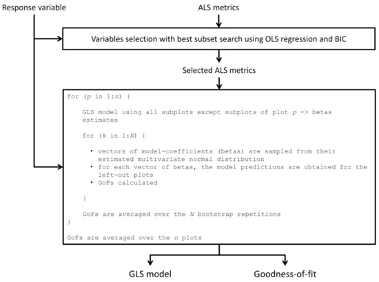
Figure 2.
Architecture of the modelling procedure.
3.3.2. Screening the Optech Titan Intensity Information
An exploratory analysis was carried out to check the linear correlation among the four forest characteristics and the mean intensity values of the three Optech Titan channels. The motivation for this analysis is the fact that, in some previous studies, it was shown that some spectral bands of passive sensors are linearly correlated to some of the response variables [28] and, thus, it is important to understand if the same happens for the Optech Titan intensity information. This analysis was carried out by producing and visually inspecting scatterplots among the response variables and the mean intensity of the three channels, and computing the coefficient of determination among them.
3.3.3. ALS Metrics Selection
Despite the hierarchical structure of our data, the metrics selection was performed using all the metrics described above and considering OLS regression models [29]. To stabilize the variance and to strengthen the linear correlation between responses and predictors, a natural logarithmic transformation was applied to the responses. The general regression model was formulated as:
where is the response for the ith sub-plot in the jth plot, is the vector of ALS metrics for the ith sub-plot in the jth plot, is the vector of model coefficients with as the intercept, and are i.i.d errors, For selecting the ALS metrics for each model, we used a best subsets search routine with sequential replacement implemented in the R package leaps [30], and the two best candidate models were retained after ranking the outputs according to the Bayes Information Criterion (BIC). Then, residual analyses were performed for each of the two candidate models to check if the models exhibit any lack-of-fit. Finally, only one model was selected as being the most appropriate for a particular forest characteristic.
3.3.4. Predictive Modelling
Using the selected ALS metrics from the OLS analysis, we re-fit the regression models using GLS regression following the protocols described in [29]. The presence of heteroscedasticity was addressed by assuming a cluster-level variance model , where the parameter is unrestricted and allows the variance of the jth plot to increase or decrease as a function of the covariates [31]. For each model, the variance function covariates were selected as the model covariates minimizing the Akaike criterion. The plot-level correlation among the sub-plots was specified using a compound symmetry structure with variance components if , and if . The models were fitted using the gls function in the nlme package [31] of R using restricted maximum likelihood estimation. A ratio estimation procedure [32] was used to adjusted the downward bias resulting after back-transforming the model predictions to original scales.
3.3.5. Model Validation
The prediction performance of the GLS models was assessed using three goodness-of-fit (GoF) criteria: (i) the predicted mean residual error sum of squares (mPRESS) defined as the PRESS statistic divided by the sample size (the same for all models); (ii) the mean deviation (MD); and (iii) the mean absolute deviation (MAD) of the prediction errors. Due to the nested structure of our dataset and considering the 12 plots as independent, the GoFs were obtained by applying a leave-one-plot-out cross-validation (LOPOCV) procedure [33]. During LOPOCV, we did not repeat the metrics selection procedure, such that our cross-validation approach did not account for any potential errors caused by model mis-specification. The ALS metrics selected in the OLS analysis using the entire sample dataset (44 sub-plots) in Section 3.3.3 were also used as predictors for each cross-validation training sample.
The dependencies among the sub-plot-level predictions do not affect the calculation of the MD and MAD criteria (which are averages), but the residual sum of squares (for calculating the mPRESS statistic) assumes independent residual errors. In order to bypass the lack of independence of the sub-plot predictions when calculating mPRESS, we opted for a parametric bootstrap (PB) procedure that worked as follows: First, the models were fitted to each training sample during LOPOCV to estimate the GLS model coefficients and their covariances. If the model assumptions are not grossly violated, the estimated intercepts and slopes of each model follow a multivariate normal distribution which is centred on the estimated coefficients and has a variance structure given by the estimated variance-covariance of the model coefficients. Sampling from the multivariate normal distributions obtained for each model, we generated vectors of coefficients to predict on the left-out observations. Note that for the PB approach to work, it was essential that the variance-covariance matrices of the model coefficients were estimated using an appropriate fitting procedure, such as GLS.
For each model, N = 250 bootstrap samples were generated, and for the kth PB sample, the mean LOPOCV prediction error was obtained as:
where n is the number of plots (12), m is the number of sub-plots (two or four, depending on the size of the original plot: 1000 m2 or 500 m2), and is the model prediction for the ith sub-plot in the jth plot under LOPOCV.
The cross-validation results relative to the arithmetic sample mean , i.e., the mPRESS statistic , mean absolute deviation , and mean deviation were obtained as:
4. Results
4.1. Screening the Optech Titan Intensity Information
In Figure 3, the correlations between the mean intensity values of each Optech Titan channels and the four response variables are displayed. The AGBha is the most correlated with the intensity values. In particular, it is negatively correlated with the mean intensity values of channel 1 (1550 nm; R2 = 0.57) and channel 3 (532 nm; R2 = 0.52). The correlation with the mean intensity values of channel 1 (1064 nm) is quite low (R2 = 0.32). The GiniDBHs seems to be uncorrelated with the intensity metrics (R2 of 0). The largest correlation for SDI is with the mean intensity value of channel 1 (1550 nm; R2 = 0.31), while for Nha the largest correlation was observed for the mean intensity value of channel 2 (1064 nm; R2 = 0.39).
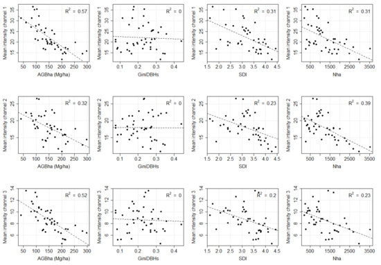
Figure 3.
Scatterplots of the response variables and the mean intensity of each Optech Titan channel for each sub-plot.
4.2. ALS Metrics Selection
In Table 4, the selected models fitted for each set of metrics and for each response variable are displayed. The GiniDBHs models were based only on elevation metrics, while the SDI and Nha models were always based on both elevation and intensity metrics. The AGBha TITAN_1_2_3 and TITAN_2 models are based only on elevation metrics, while the others contain both sets of metrics. The TITAN_3 model for the prediction of GiniDBHs was only based on one metric. The indices extracted from Titan intensities were selected only for Nha. The most frequently selected intensity metrics was the sum of intensities (itot). Regarding the elevation metrics there was more variation in the selection even if the cumulative percentage of returns (zpcumN) and the z percentiles (zqN) were present in almost all the models.
Table 4.
Metrics selected in each set of metrics and for each response variable.
4.3. Models Validation
As can be seen in Table 5, the most accurate models for the AGBha, GiniDBHs, and Nha prediction were the TITAN_1_2_3, while for the SDI it was the ALS70. The ALS70 data resulted in the best model only for the SDI prediction. In this case, the results were, in fact, quite similar to those of the TITAN and TITAN_2 models. The TITAN_3 models were always the least accurate. In Figure 4, Figure 5, Figure 6 and Figure 7, scatterplots of predicted versus observed values can be seen. The TITAN_1_2_3 model provided the best results. Regarding the Nha, it is clear that all the models had more difficulties in predicting high Nha values compared to low Nha values. The TITAN_3 model failed totally in capturing the variation of the GiniDBHs values.
Table 5.
Models’ goodness-of-fit: (i) mean residual error sum of squares (mPRESS) defined as the PRESS statistic divided by the sample size (the same for all models); (ii) the mean absolute deviation (MAD); and (iii) the mean deviation (MD).
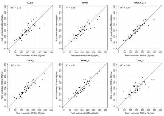
Figure 4.
Scatterplots of the field-estimated and ALS-predicted values of aboveground biomass per hectare (AGBha) for each sub-plot for each model. In each scatterplot the Pearson’s correlation coefficient between observed and predicted values is n.
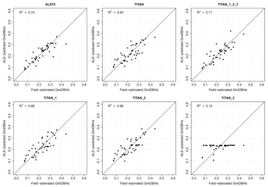
Figure 5.
Scatterplots of the field-estimated and ALS-predicted values of Gini coefficient of DBHs (GiniDBHs) for each sub-plot for each model. In each scatterplot the Pearson’s correlation coefficient between observed and predicted values is shown.
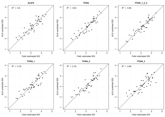
Figure 6.
Scatterplots of the field-estimated and ALS-predicted values of the Shannon diversity index (SDI) for each sub-plot for each model. In each scatterplot the Pearson’s correlation coefficient between the observed and predicted values is shown.
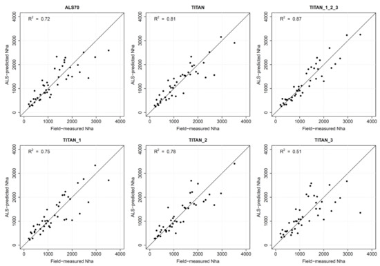
Figure 7.
Scatterplots of the field-estimated and ALS-predicted values of the number of trees per hectare (Nha) for each sub-plot for each model. In each scatterplot the Pearson’s correlation coefficient between observed and predicted values is shown.
5. Discussion
The AGBha is the most correlated with the mean intensity values. Similar behaviour was reported in previous studies relating aboveground biomass with Landsat 8 bands, but with a lower correlation [28]. Channel 1 (1550 nm) showed the largest correlation, confirming similar results obtained with passive multi/hyperspectral sensors [34,35]. The smaller correlation between the channel 2 (1064 nm) mean intensity value and AGBha may be due to the channel’s correlation with the green leaf density and the fact that some of the sub-plots have sparse forest that can influence its values. The GiniDBHs was not correlated with any of the intensity metrics, and this can be explained by the fact that the DBH is generally more related to the elevation information than the spectral information. The SDI and Nha showed a small correlation with channel 1 (1550 nm) and channel 2 (1064 nm). This is also in line with results reported in the literature with passive multi/hyperspectral sensors. Thus, a general inference seems to be that having two additional channels in the medium infrared and green parts of the spectrum tends to improve the prediction capabilities of ALS sensors.
The fact that the models based on the multispectral ALS sensor always gave better results than those based on the standard single-channel ALS data shows that these data are a good source of information to predict the considered forest characteristics. If we consider the data of channel 2 of the Optech Titan as reference (TITAN_2 models), it can be seen that there was always an improvement by using the other Titan channels as an addition. This is an important observation as it is shows that even if a conventional ALS sensor is already providing good results, these results can be further improved with the addition of the other two spectral channels.
The ALS70 data can only be considered as a baseline for comparison since other factors not accounted for in this study may influence the results. Indeed, the two acquisitions were carried out at two different points in time, with different flying and instrument settings. The flying altitude, the day of acquisition, and the scan angle differed between the two acquisitions. Indeed, the results of the ALS70 models and the TITAN_2 models, both based on data acquired at the same wavelength, frequently provided different results. In this case, the acquisition conditions, the different point densities, and settings were probably causes by these differences. Moreover the two datasets were acquired in different seasons: the ALS70 were acquired at the end of the summer (leaf-on conditions), while the Optech Titan data in the spring (mainly leaf-off conditions). This last factor may have influenced the results, even if deciduous trees are absent in about half of the subplots and, in total, they represent only 22% of the trees inside the plots.
The different channels did not provide the same amount of information and the multispectral information was not always used. In particular, for the AGBha models, it seemed that the elevation information was much more useful. In contrast, the intensity information was used frequently for the SDI. This is a logical finding as AGBha is strongly related to the height of the trees, which is well represented by the elevation information, while the SDI quantifying the species diversity is better captured by spectral information, which may help distinguish different species with differences in reflectance in various parts of the electromagnetic spectrum.
The fact that channel 3 (532 nm) seemed to be the least correlated with the analysed response variables (Figure 3) and that the metrics derived from channel 3 data were, in general, the least frequently selected in the regression models (Table 4) was as expected. The channel 3 (532 nm) data are, in general, considered more noisy compared to the other channels due to the fact that it is working in the visible range of light and it has a beam divergence that is twice as large compared to the other two channels. For this channel we also had the smallest point density in the 12 study plots, i.e., 3 pts/m2 versus 21 pts/m2 of channel 2 (1064 nm).
The indices computed from the intensity values of the three channels of the Optech Titan sensor seemed to add little as predictors. They were chosen only in one model. Despite this, we think that it is, in any case, important to have the possibility to calculate such indices from ALS data as they might be more useful for other applications and response variables than those considered in the current study. As an example, Karila et al. (2017) showed that the pseudo-NDVI computed from the Optech Titan channels can be useful for accurate road mapping. In the future, it would be interesting to compare such indices to those obtained from satellite optical data over forested areas.
6. Conclusions
Multispectral ALS data were shown to be a useful source of information for the prediction of the four forest characteristics addressed in this study. Moreover, multispectral ALS models provided better model prediction results compared to ALS data acquired with a conventional ALS working at 1064 nm. Among the new additional spectral channels, as compared to conventional ALS instruments, channel 1 (1550 nm) seemed the most useful as it showed a good correlation with almost all the considered response variables. Channel 3 (532 nm) seemed to provide less informative data. We think that the potential of multispectral ALS data in forestry and ecological applications is great. However, more studies with larger and more diverse datasets with respect to response variables and environmental conditions are needed to fully explore the potential of these state-of the art multispectral ALS instruments.
Acknowledgments
This work was supported by the HyperBio project (project #244599), which was financed by the BIONÆR program of the Research Council of Norway and by TerraTec AS, Norway.
Author Contributions
M.D., L.T.E., and D.G. conceived and designed the experiments; M.D. and L.T.E. performed the experiments; M.D. and L.T.E. analyzed the data; T.G. and E.N. provided the data; M.D. and L.T.E. wrote the paper; and T.G., E.N., and D.G. revised the manuscript before submission.
Conflicts of Interest
The authors declare no conflict of interest.
References
- Maltamo, M.; Naesset, E.; Vauhkonen, J. Forestry Applications of Airborne Laser Scanning; Springer: Berlin/Heidelberg, Germany, 2014; ISBN 9789401786621. [Google Scholar]
- Schwarz, B. Lidar: Mapping the world in 3D. Nat. Photonics 2010, 4, 429–430. [Google Scholar] [CrossRef]
- Nilsson, M. Estimation of tree heights and stand volume using an airborne lidar system. Remote Sens. Environ. 1996, 56, 1–7. [Google Scholar] [CrossRef]
- Næsset, E. Determination of mean tree height of forest stands using airborne laser scanner data. ISPRS J. Photogramm. Remote Sens. 1997, 52, 49–56. [Google Scholar] [CrossRef]
- Næsset, E. Estimating timber volume of forest stands using airborne laser scanner data. ISPRS J. Photogramm. Remote Sens. 1997, 61, 246–253. [Google Scholar] [CrossRef]
- Maltamo, M.; Næsset, E.; Vauhkonen, J. Forestry Applications of Airborne Laser Scanning; Maltamo, M., Næsset, E., Vauhkonen, J., Eds.; Managing Forest Ecosystems; Springer: Dordrecht, The Netherlands, 2014; Volume 27, ISBN 978-94-017-8662-1. [Google Scholar]
- Lone, K.; van Beest, F.M.; Mysterud, A.; Gobakken, T.; Milner, J.M.; Ruud, H.-P.; Loe, L.E. Improving broad scale forage mapping and habitat selection analyses with airborne laser scanning: The case of moose. Ecosphere 2014, 5, art144. [Google Scholar] [CrossRef]
- Lone, K.; Loe, L.E.; Gobakken, T.; Linnell, J.D.C.; Odden, J.; Remmen, J.; Mysterud, A. Living and dying in a multi-predator landscape of fear: Roe deer are squeezed by contrasting pattern of predation risk imposed by lynx and humans. Oikos 2014, 123, 641–651. [Google Scholar] [CrossRef]
- Loarie, S.R.; Tambling, C.J.; Asner, G.P. Lion hunting behaviour and vegetation structure in an African savanna. Anim. Behav. 2013, 85, 899–906. [Google Scholar] [CrossRef]
- Bouvier, M.; Durrieu, S.; Gosselin, F.; Herpigny, B. Use of airborne lidar data to improve plant species richness and diversity monitoring in lowland and mountain forests. PLoS ONE 2017, 12, e0184524. [Google Scholar] [CrossRef] [PubMed]
- Ørka, H.O.; Næsset, E.; Bollandsås, O.M. Classifying species of individual trees by intensity and structure features derived from airborne laser scanner data. Remote Sens. Environ. 2009, 113, 1163–1174. [Google Scholar] [CrossRef]
- Chen, B.; Shi, S.; Gong, W.; Zhang, Q.; Yang, J.; Du, L.; Sun, J.; Zhang, Z.; Song, S. Multispectral LiDAR Point Cloud Classification: A Two-Step Approach. Remote Sens. 2017, 9, 373. [Google Scholar] [CrossRef]
- Sun, J.; Shi, S.; Gong, W.; Yang, J.; Du, L.; Song, S.; Chen, B.; Zhang, Z. Evaluation of hyperspectral LiDAR for monitoring rice leaf nitrogen by comparison with multispectral LiDAR and passive spectrometer. Sci. Rep. 2017, 7, 40362. [Google Scholar] [CrossRef] [PubMed]
- Hakala, T.; Suomalainen, J.; Kaasalainen, S.; Chen, Y. Full waveform hyperspectral LiDAR for terrestrial laser scanning. Opt. Express 2012, 20, 7119. [Google Scholar] [CrossRef] [PubMed]
- Puttonen, E.; Suomalainen, J.; Hakala, T.; Räikkönen, E.; Kaartinen, H.; Kaasalainen, S.; Litkey, P. Tree species classification from fused active hyperspectral reflectance and LIDAR measurements. For. Ecol. Manag. 2010, 260, 1843–1852. [Google Scholar] [CrossRef]
- Danson, F.M.; Gaulton, R.; Armitage, R.P.; Disney, M.; Gunawan, O.; Lewis, P.; Pearson, G.; Ramirez, A.F. Developing a dual-wavelength full-waveform terrestrial laser scanner to characterize forest canopy structure. Agric. For. Meteorol. 2014, 198–199, 7–14. [Google Scholar] [CrossRef]
- Budei, B.C.; St-Onge, B.; Hopkinson, C.; Audet, F.-A. Identifying the genus or species of individual trees using a three-wavelength airborne lidar system. Remote Sens. Environ. 2017. [Google Scholar] [CrossRef]
- Karila, K.; Matikainen, L.; Puttonen, E.; Hyyppa, J. Feasibility of Multispectral Airborne Laser Scanning Data for Road Mapping. IEEE Geosci. Remote Sens. Lett. 2017, 14, 294–298. [Google Scholar] [CrossRef]
- McIver, C.A.; Metcalf, J.P.; Olsen, R.C. Spectral LiDAR analysis for terrain classification. Proc. SPIE 2017, 10191, 101910J. [Google Scholar]
- Axelsson, A.; Lindberg, E.; Olsson, H. Exploring Multispectral ALS Data for Tree Species Classification. Remote Sens. 2018, 10, 183. [Google Scholar] [CrossRef]
- Fernandez-Diaz, J.C.; Carter, W.E.; Glennie, C.; Shrestha, R.L.; Pan, Z.; Ekhtari, N.; Singhania, A.; Hauser, D.; Sartori, M. Capability assessment and performance metrics for the titan multispectral mapping lidar. Remote Sens. 2016, 8, 936. [Google Scholar] [CrossRef]
- Yu, X.; Hyyppä, J.; Litkey, P.; Kaartinen, H.; Vastaranta, M.; Holopainen, M. Single-Sensor Solution to Tree Species Classification Using Multispectral Airborne Laser Scanning. Remote Sens. 2017, 9, 108. [Google Scholar] [CrossRef]
- Asner, G.P.; Mascaro, J. Mapping tropical forest carbon: Calibrating plot estimates to a simple LiDAR metric. Remote Sens. Environ. 2014, 140, 614–624. [Google Scholar] [CrossRef]
- Mauya, E.W.; Ene, L.T.; Bollandsås, O.M.; Gobakken, T.; Næsset, E.; Malimbwi, R.E.; Zahabu, E. Modelling aboveground forest biomass using airborne laser scanner data in the miombo woodlands of Tanzania. Carbon Balance Manag. 2015, 10, 28. [Google Scholar] [CrossRef] [PubMed]
- Valbuena, R.; Eerikäinen, K.; Packalen, P.; Maltamo, M. Gini coefficient predictions from airborne lidar remote sensing display the effect of management intensity on forest structure. Ecol. Indic. 2016, 60, 574–585. [Google Scholar] [CrossRef]
- Marklund, L.G. Biomass Functions for Pine, Spruce and Birch in Sweden; FAO: Rome, Italy, 1988. [Google Scholar]
- Korpela, I.; Ørka, H.O.; Hyyppä, J.; Heikkinen, V.; Tokola, T. Range and AGC normalization in airborne discrete-return LiDAR intensity data for forest canopies. ISPRS J. Photogramm. Remote Sens. 2010, 65, 369–379. [Google Scholar] [CrossRef]
- Gizachew, B.; Solberg, S.; Næsset, E.; Gobakken, T.; Bollandsås, O.M.; Breidenbach, J.; Zahabu, E.; Mauya, E.W. Mapping and estimating the total living biomass and carbon in low-biomass woodlands using Landsat 8 CDR data. Carbon Balance Manag. 2016, 11, 13. [Google Scholar] [CrossRef] [PubMed]
- Zuur, A.F.; Ieno, E.N.; Walker, N.; Saveliev, A.A.; Smith, G.M. Mixed Effects Models and Extensions in Ecology with R; Statistics for Biology and Health; Springer: New York, NY, USA, 2009; ISBN 978-0-387-87457-9. [Google Scholar]
- Lumley, T. Package “leaps”: Regression Subset Selection 2017. Available online: https://cran.r-project.org/web/packages/leaps/leaps.pdf (accessed on 9 April 2018).
- Pinheiro, J.; Bates, D.; DebRoy, S.; Sarkar, D.; Heisterkamp, S.; Van Willigen, B. nlme: Linear and Nonlinear Mixed Effects Models. 2017. Available online: https://cran.r-project.org/web/packages/nlme/nlme.pdf (accessed on 9 April 2018).
- Snowdon, P. A ratio estimator for bias correction in logarithmic regressions. Can. J. For. Res. 1991, 21, 720–724. [Google Scholar] [CrossRef]
- Roberts, D.R.; Bahn, V.; Ciuti, S.; Boyce, M.S.; Elith, J.; Guillera-Arroita, G.; Hauenstein, S.; Lahoz-Monfort, J.J.; Schröder, B.; Thuiller, W.; et al. Cross-validation strategies for data with temporal, spatial, hierarchical, or phylogenetic structure. Ecography 2017, 40, 913–929. [Google Scholar] [CrossRef]
- Hall, R.J.; Skakun, R.S.; Arsenault, E.J.; Case, B.S. Modeling forest stand structure attributes using Landsat ETM+ data: Application to mapping of aboveground biomass and stand volume. For. Ecol. Manag. 2006, 225, 378–390. [Google Scholar] [CrossRef]
- Gerylo, G.R.; Hall, R.J.; Franklin, S.E.; Smith, L. Empirical relations between Landsat TM spectral response and forest stands near Fort Simpson, Northwest Territories, Canada. Can. J. Remote Sens. 2002, 28, 68–79. [Google Scholar] [CrossRef]
© 2018 by the authors. Licensee MDPI, Basel, Switzerland. This article is an open access article distributed under the terms and conditions of the Creative Commons Attribution (CC BY) license (http://creativecommons.org/licenses/by/4.0/).