A Combined Approach to Classifying Land Surface Cover of Urban Domestic Gardens Using Citizen Science Data and High Resolution Image Analysis


Abstract
1. Introduction
2. Materials and Methods
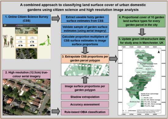
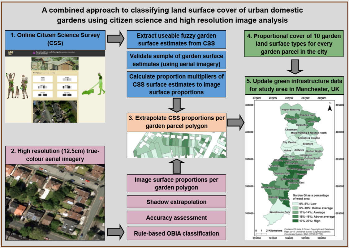
2.1. Overview
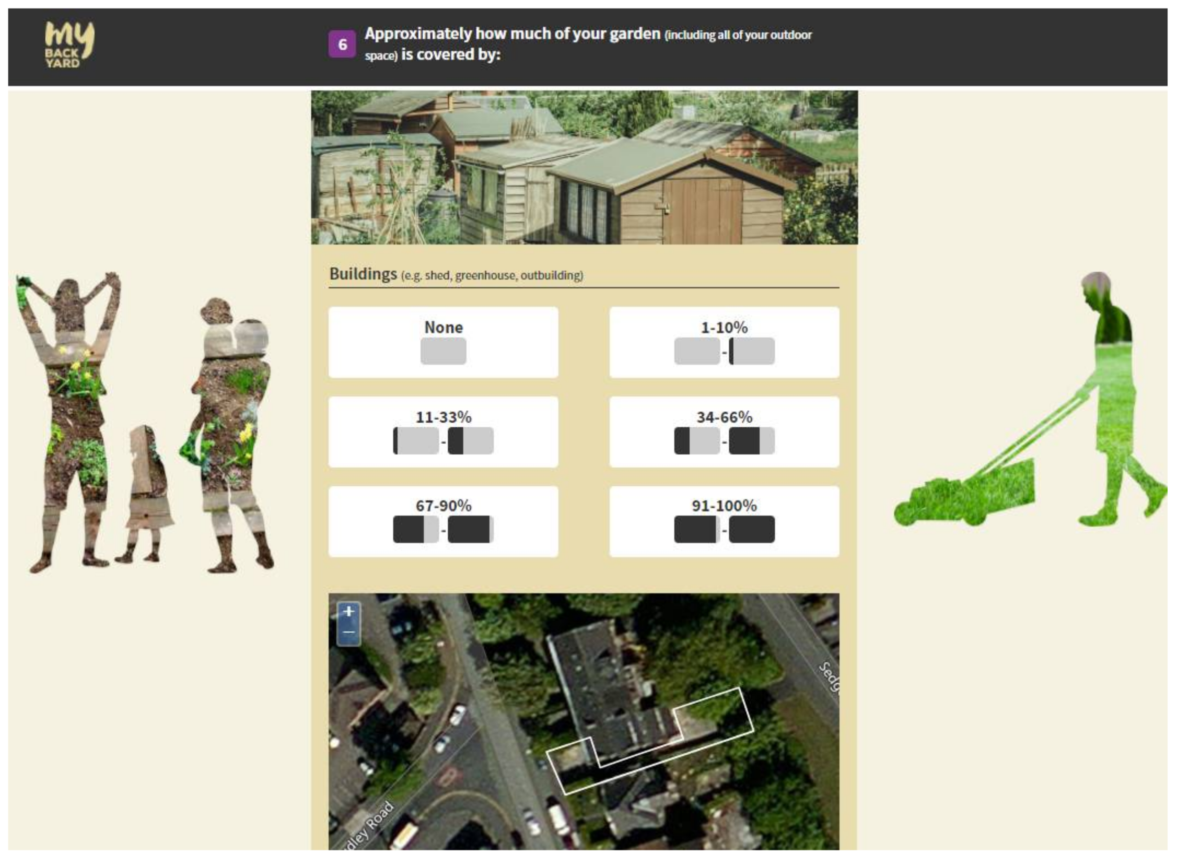
2.2. Online Citizen Science Survey Tool: My Back Yard
- To gather the proportional land surface cover and exact spatial location of the garden, i.e., the respondent enters their postcode; the tool uses this to determine the boundary of the space-based upon Ordnance Survey mapping; the respondent confirms this or corrects it using spatial editing and selection tools on the map.
- To allow the respondent (and other users) to explore the data already collected, in a generalised form, so that they can see their own contribution in the context of their neighbourhood, and learn about the benefits of green and blue space.
2.3. Extension of the Citizen Science Survey (CSS) Surface Estimations
2.3.1. Data
2.3.2. Validation of Citizen Science Survey Land Surface Estimations
2.3.3. Classification
Separation into Super-Classes
Identification of Tree Canopy Objects
Classification of Grass and Shrubs
Classification Optimisation
Building Classification
Accuracy Assessment
Extrapolation within Shadow Class
3. Results
3.1. Citizen Science Survey Responses
3.2. Validation of Garden Composition Derived from the Citizen Science Survey
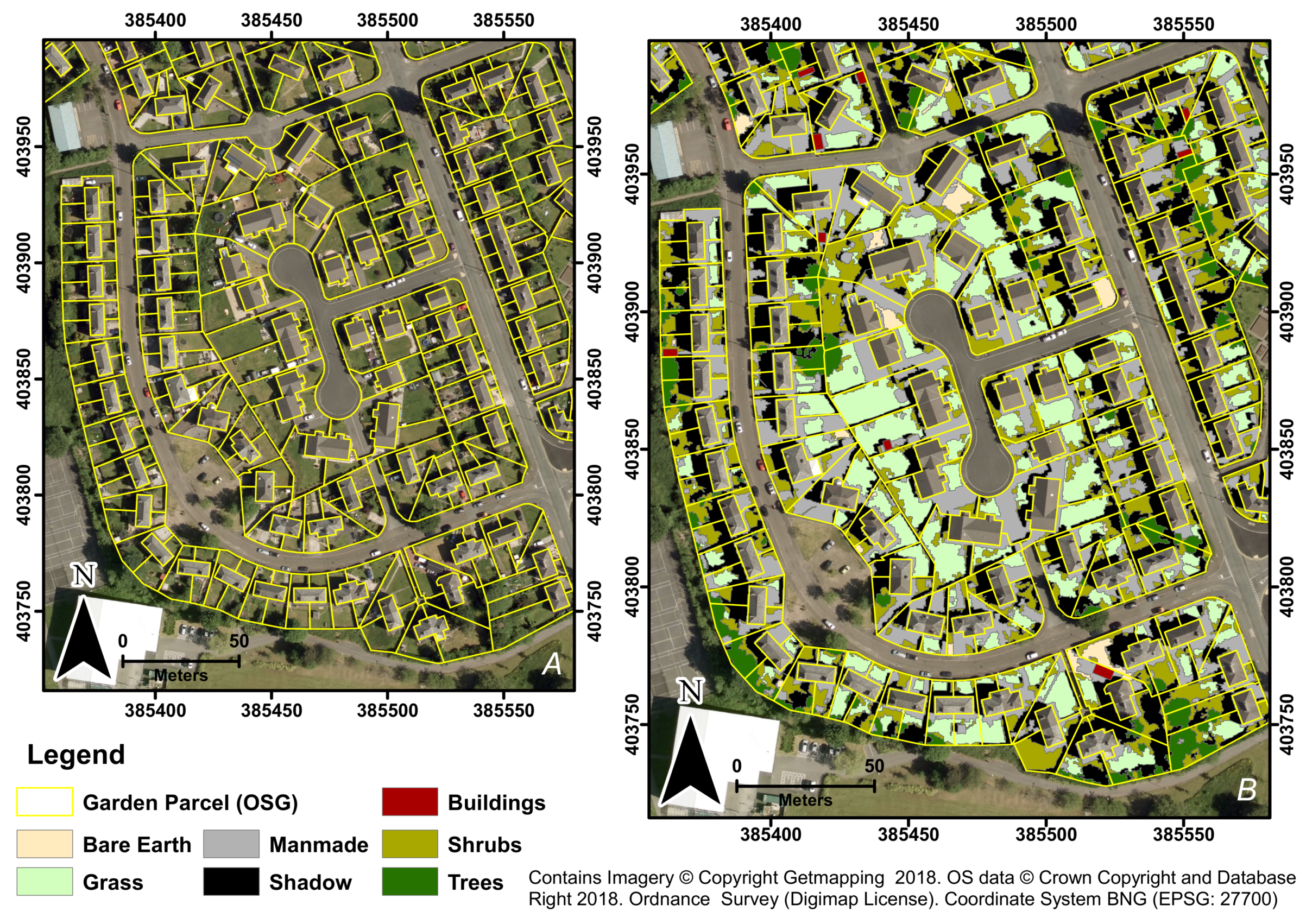
Image Classification
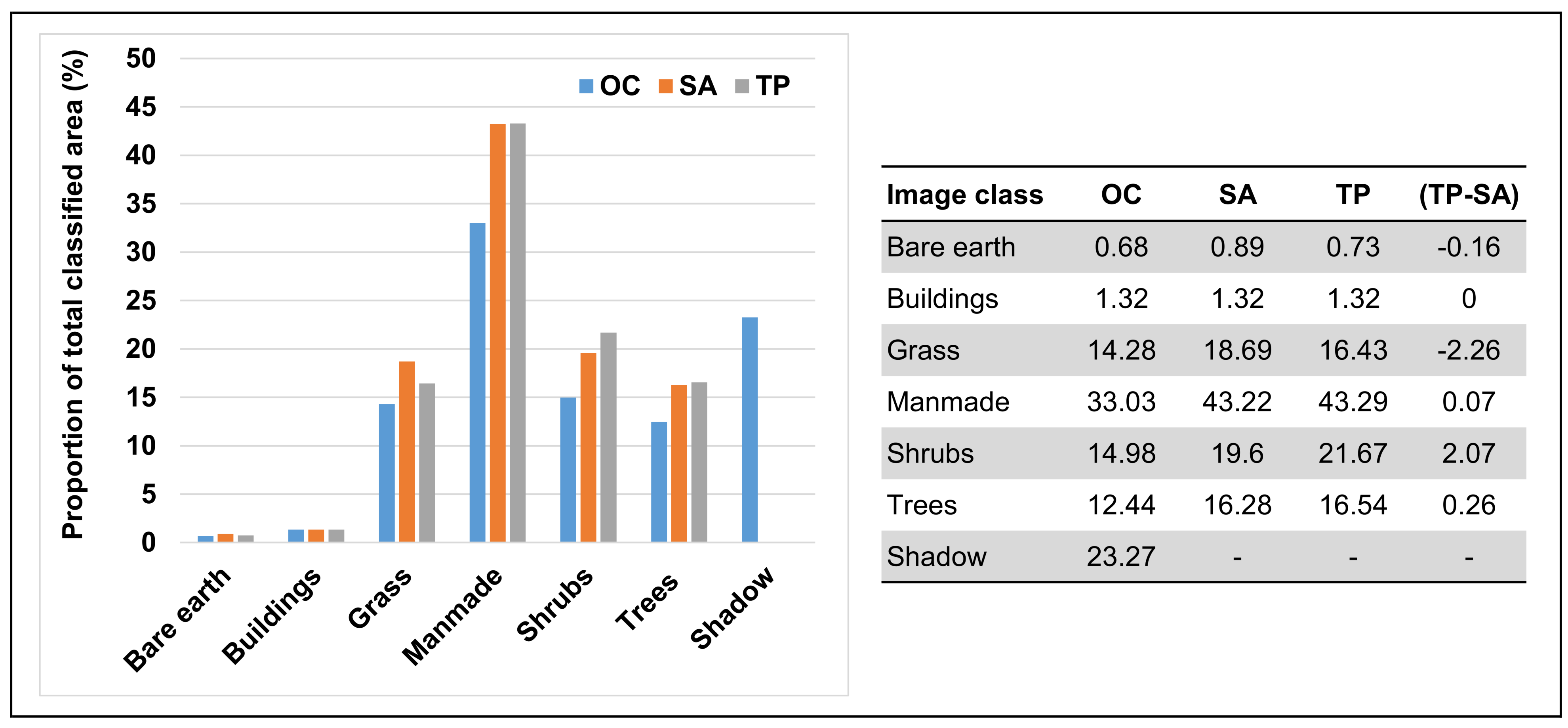
3.3. Extrapolation of CSS Surface Proportions to Classified Data
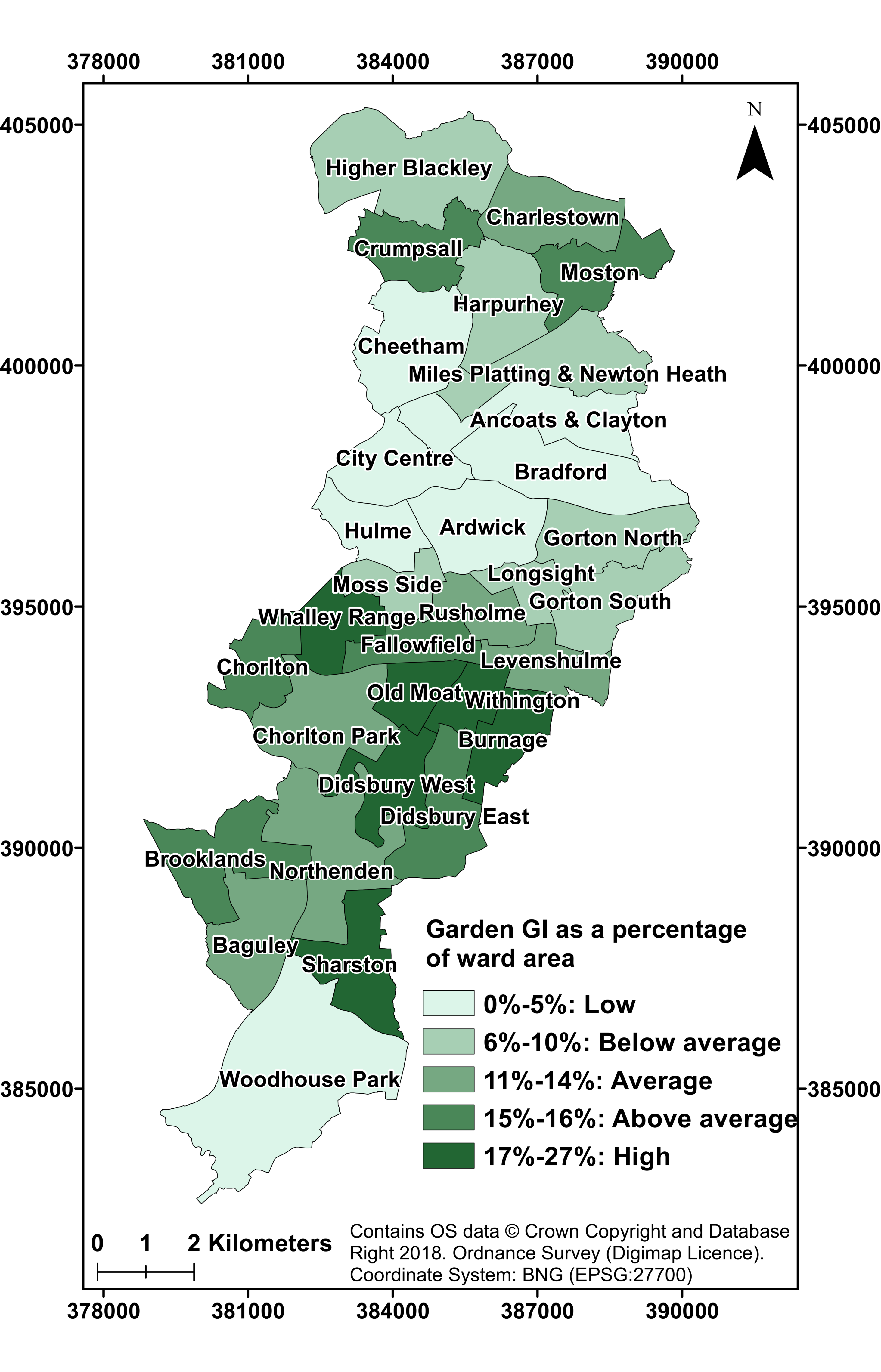
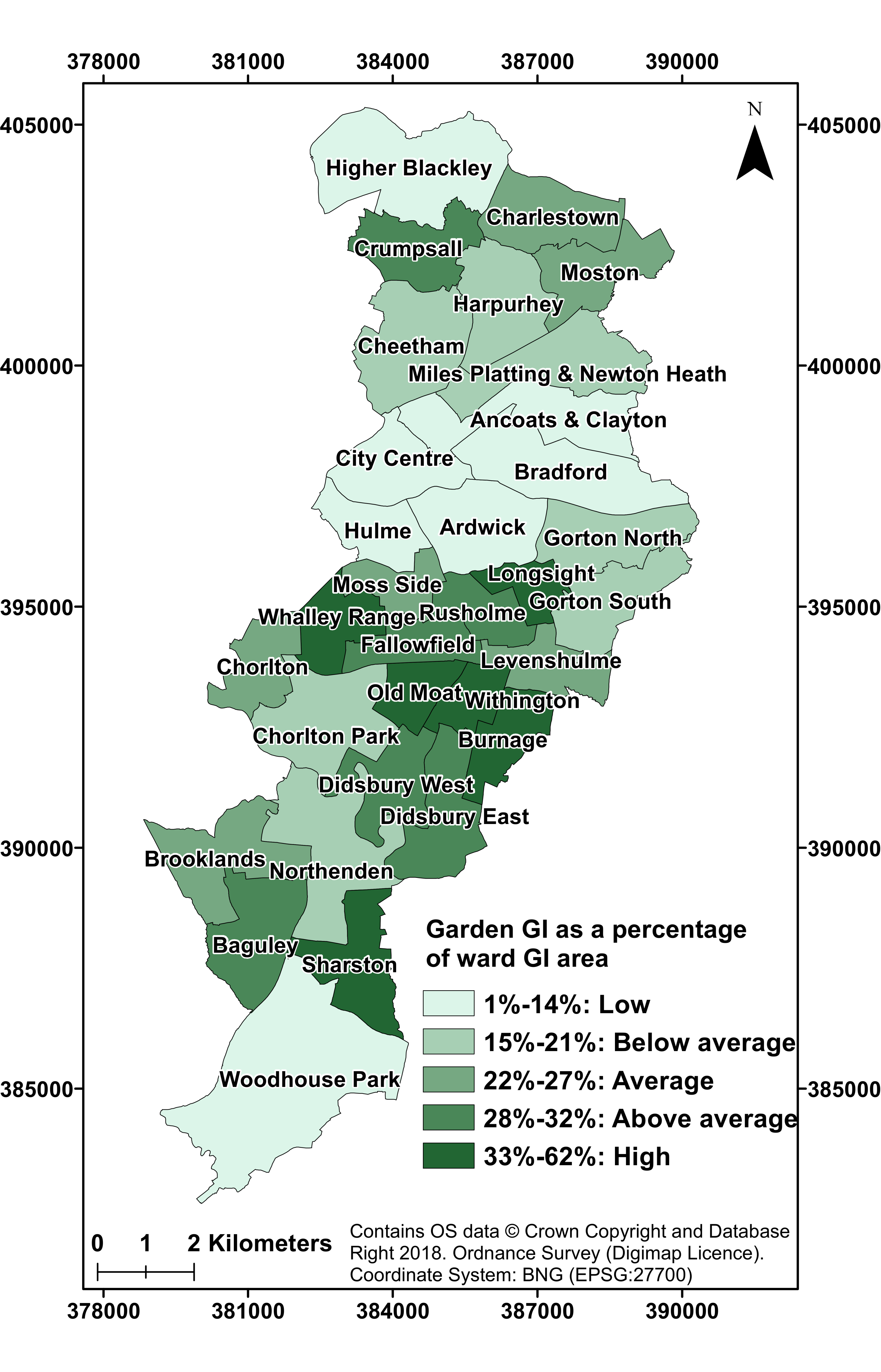
3.4. Green Infrastructure (GI) in Manchester’s Gardens
4. Discussion
5. Conclusions
Supplementary Materials
Acknowledgments
Author Contributions
Conflicts of Interest
References
- Mathieu, R.; Freeman, C.; Aryal, J. Mapping private gardens in urban areas using object-oriented techniques and very high resolution imagery. Landsc. Urban Plan. 2007, 81, 179–192. [Google Scholar] [CrossRef]
- Warhurst, J.R.; Parks, K.E.; McCulloch, L.; Hudson, M.D. Front gardens to car parks: Changes in garden permeability and effects on flood regulation. Sci. Total Environ. 2014, 485, 329–339. [Google Scholar] [CrossRef] [PubMed]
- Cameron, R.W.F.; Blanuša, T.; Taylor, J.E.; Salisbury, A.; Halstead, A.J.; Henricot, B.; Thompson, K. The domestic garden–Its contribution to urban green infrastructure. Urban For. Urban Green. 2012, 11, 129–137. [Google Scholar] [CrossRef]
- Newman, G.; Chandler, M.; Clyde, M.; McGreavy, B.; Haklay, M.; Ballard, H.; Gray, S.; Scarpino, R.; Hauptfeld, R.; Mellor, D.; et al. Leveraging the power of place in citizen science for effective conservation decision making. Biol. Conserv. 2017, 208, 55–64. [Google Scholar] [CrossRef]
- Loram, A.; Warren, P.; Thompson, K.; Gaston, K. Urban domestic gardens: The effects of human interventions on garden composition. Environ. Manag. 2011, 48, 808–824. [Google Scholar] [CrossRef] [PubMed]
- Lin, B.B.; Gaston, K.J.; Fuller, R.A.; Wu, D.; Bush, R.; Shanahan, D.F. How green is your garden? Urban form and socio-demographic factors influence yard vegetation, visitation, and ecosystem service benefits. Landsc. Urban Plan. 2017, 157, 239–246. [Google Scholar] [CrossRef]
- DCLG, Department for Communities and Local Government (DCLG). Guidance on the Permeable Surfacing of Front Gardens. 2008. Available online: https://www.gov.uk/government/uploads/system/uploads/attachment_data/file/7728/pavingfrontgardens.pdf (accessed on 12 February 2018).
- Perry, T.; Nawaz, R. An investigation into the extents and impacts of hard surfacing of domestic gardens in an area of Leeds, United Kingdom. Landsc. Urban Plan. 2008, 86, 1–13. [Google Scholar] [CrossRef]
- Ghosh, S.; Head, L. Retrofitting the suburban garden: Morphologies and some elements of two Australian residential suburbs compared. Aust. Geogr. 2009, 40, 319–346. [Google Scholar] [CrossRef]
- Sayce, S.; Walford, N.; Garside, P. Residential development on gardens in England: Their role in providing sustainable housing supply. Land Use Policy 2012, 29, 771–780. [Google Scholar] [CrossRef]
- Hof, A.; Wolf, N. Estimating potential outdoor water consumption in private and urban landscapes by coupling high-resolution image analysis, irrigation water needs and evaporation estimation in Spain. Landsc. Urban Plan. 2014, 123, 61–72. [Google Scholar] [CrossRef]
- Cameron, R.W.; Blanusa, T. Green infrastructure and ecosystem services—Is the devil in the detail? Ann. Bot. Lond. 2016, 118, 377–391. [Google Scholar] [CrossRef] [PubMed]
- Gill, S.E.; Handley, J.F.; Ennos, A.R.; Pauleit, S. Adapting cities for climate change: The role of green infrastructure. Built Environ. 2007, 33, 115–133. [Google Scholar] [CrossRef]
- Hall, J.M.; Handley, J.F.; Ennos, A.R. The potential of tree planting to climate proof high density residential areas in Manchester, UK. Landsc. Urban Plan. 2012, 104, 410–417. [Google Scholar] [CrossRef]
- Armson, D.; Stringer, P.; Ennos, A.R. The effect of tree shade and grass on surface and globe temperatures in an urban area. Urban For. Urban Green. 2012, 11, 245–255. [Google Scholar] [CrossRef]
- Dennis, M.; Barlow, D.; Cavan, G.; Cook, P.A.; Gilchrist, A.; Handley, J.; James, P.; Thompson, J.; Tzoulas, K.; Wheater, C.P.; et al. Mapping urban green infrastructure: A novel landscape-based approach to incorporating land use and land cover in the mapping of human-dominated systems. Land 2018, 7, 17. [Google Scholar] [CrossRef]
- Kazmierczak, A.; Cavan, G. Surface water flooding risk to urban communities: Analysis of vulnerability, hazard & exposure. Landsc. Urban Plan. 2011, 103, 185–197. [Google Scholar]
- Smith, C.L.; Lawson, N. Identifying Extreme Event Climate Thresholds for Greater Manchester, UK: Examining the Past to Prepare for the Future. Meteorol. Appl. 2012, 19, 26–35. [Google Scholar] [CrossRef]
- Carter, J.G.; Cavan, G.; Connelly, A.; Guy, S.; Handley, J.; Kazmierczak, A. Climate change and the city: Building capacity for urban adaptation. Prog. Plan. 2014, 95, 1–66. [Google Scholar] [CrossRef]
- Levermore, G.J.; Parkinson, J.B.; Laycock, P.J.; Lindley, S.J. The Urban Heat Island in Manchester 1996–2011. Build. Serv. Eng. Res. Technol. 2015, 36, 343–356. [Google Scholar] [CrossRef]
- Intelligence Hub (Manchester Statistics) Mid-Year Population Estimates for Manchester, ONS, Crown Copyright. Available online: https://dashboards.instantatlas.com/viewer/report?appid=9853f1a1b412404b806dab4d1918def7 (accessed on 12 February 2018).
- AGMA, Association of Greater Manchester Authorities. Greater Manchester Strategic Housing Market Assessment, 2010. Available online: http://www.manchester.gov.uk/download/downloads/id/14074/gm_strategic_housing_market_assessment_shma_update_may_2010.pdf (accessed on 12 February 2018).
- Brown, G. An empirical evaluation of the spatial accuracy of public participation GIS (PPGIS) data. Appl. Geogr. 2012, 34, 289–294. [Google Scholar] [CrossRef]
- Getmapping, Aerial Data—High Resolution Imagery. Available online: http://www.getmapping.com/products-and-services/aerial-imagery-data/aerial-data-high-resolution-imagery (accessed on 29 March 2018).
- City of Trees (Greater Manchester Tree Audit, Manchester, UK). Personal communication, 2011.
- Novack, T.; Esch, T.; Kux, H.; Stilla, U. Machine learning comparison between WorldView-2 and QuickBird-2-simulated imagery regarding object-based urban land cover classification. Remote Sens. 2011, 3, 2263–2282. [Google Scholar] [CrossRef]
- Lu, D.; Weng, Q. A survey of image classification methods and techniques for improving classification performance. Int. J. Remote Sens. 2007, 28, 823–870. [Google Scholar] [CrossRef]
- Salas, E.A.L.; Boykin, K.G.; Valdez, R. Multispectral and texture feature application in image-object analysis of summer vegetation in Eastern Tajikistan Pamirs. Remote Sens. 2016, 8, 78. [Google Scholar] [CrossRef]
- Blaschke, T.; Hay, G.J.; Kelly, M.; Lang, S.; Hofmann, P.; Addink, E.; Feitosa, R.Q.; van der Meer, F.; van der Werff, G.; van Coillie, F.; et al. Geographic object-based image analysis–towards a new paradigm. ISPRS J. Photogramm. 2014, 87, 180–191. [Google Scholar] [CrossRef] [PubMed]
- Aksoy, B.; Ercanoglu, M. Landslide identification and classification by object-based image analysis and fuzzy logic: An example from the Azdavay region (Kastamonu, Turkey). Comput. Geosci. 2012, 38, 87–98. [Google Scholar] [CrossRef]
- Foody, G.M. Harshness in image classification accuracy assessment. Int. J. Remote Sens. 2008, 29, 3137–3158. [Google Scholar] [CrossRef]
- Huang, X.; Zhang, L. An SVM ensemble approach combining spectral, structural, and semantic features for the classification of high-resolution remotely sensed imagery. IEEE Trans. Geosci. Remote 2013, 51, 257–272. [Google Scholar] [CrossRef]
- Feng, Q.; Liu, J.; Gong, J. UAV remote sensing for urban vegetation mapping using random forest and texture analysis. Remote Sens. 2015, 7, 1074–1094. [Google Scholar] [CrossRef]
- Shackelford, A.K.; Davis, C.H. Fully automated road network extraction from high-resolution satellite multispectral imagery. In Proceedings of the IGARSS’03, 2003 IEEE International Geoscience and Remote Sensing Symposium, Toulouse, France, 21–25 July 2003; IEEE: Piscataway, NJ, USA, 2003; Volume 1, pp. 461–463. [Google Scholar]
- Meyer, G.E.; Neto, J.C. Verification of color vegetation indices for automated crop imaging applications. Comput. Electron. Agr. 2008, 63, 282–293. [Google Scholar] [CrossRef]
- Motohka, T.; Nasahara, K.N.; Oguma, H.; Tsuchida, S. Applicability of green-red vegetation index for remote sensing of vegetation phenology. Remote Sens. 2010, 2, 2369–2387. [Google Scholar] [CrossRef]
- Definiens. Definiens Developer User Guide XD 2.0.4. 2012. Available online: www.imperial.ac.uk/media/imperial.../Definiens-Developer-User-Guide-XD-2.0.4.pdf (accessed on 18 February 2018).
- Bunting, P.; Lucas, R. The delineation of tree crowns in Australian mixed species forests using hyperspectral Compact Airborne Spectrographic Imager (CASI) data. Remote Sens. Environ. 2006, 101, 230–248. [Google Scholar] [CrossRef]
- Rampi, L.P.; Knight, J.F.; Pelletier, K.C. Wetland mapping in the upper midwest United States. Photogramm. Eng. Remote Sens. 2014, 80, 439–448. [Google Scholar] [CrossRef]
- Zhou, W.; Troy, A. An object-oriented approach for analysing and characterizing urban landscape at the parcel level. Int. J. Remote Sens. 2008, 29, 3119–3135. [Google Scholar]
- Congalton, R.G.; Green, K. Assessing the Accuracy of Remotely Sensed Data: Principles and Practices; CRC Press: Boca Raton, FL, USA, 2008. [Google Scholar]
- Zhou, W.; Huang, G.; Troy, A.; Cadenasso, M.L. Object-based land cover classification of shaded areas in high spatial resolution imagery of urban areas: A comparison study. Remote Sens. Environ. 2009, 113, 1769–1777. [Google Scholar] [CrossRef]
- Smith, R.M.; Gaston, K.J.; Warren, P.H.; Thompson, K. Urban domestic gardens (V): Relationships between landcover composition, housing and landscape. Landsc. Ecol. 2005, 20, 235–253. [Google Scholar] [CrossRef]
- Anderson, J.R. A Land Use and Land Cover Classification System for Use with Remote Sensor Data; US Government Printing Office: Washington, DC, USA, 1976; Volume 964.
- Manchester City Council (Green Infrastructure Dataset, Manchester, UK). Personal communication, 2016.
- Stehman, S.V.; Wickham, J.D. Pixels, blocks of pixels, and polygons: Choosing a spatial unit for thematic accuracy assessment. Remote Sens. Environ. 2011, 115, 3044–3055. [Google Scholar] [CrossRef]
- Comber, A.; See, L.; Fritz, S.; Van der Velde, M.; Perger, C.; Foody, G. Using control data to determine the reliability of volunteered geographic information about land cover. Int. J. Appl. Earth Obs. 2013, 23, 37–48. [Google Scholar] [CrossRef]
- Shahtahmassebi, A.; Yang, N.; Wang, K.; Moore, N.; Shen, Z. Review of shadow detection and de-shadowing methods in remote sensing. Chin. Geogr. Sci. 2013, 23, 403–420. [Google Scholar] [CrossRef]
- Yang, J.; He, Y.; Caspersen, J. Fully constrained linear spectral unmixing based global shadow compensation for high resolution satellite imagery of urban areas. Int. J. Appl. Earth Obs. Geoinform. 2015, 38, 88–98. [Google Scholar] [CrossRef]
- Mountrakis, G.; Im, J.; Ogole, C. Support vector machines in remote sensing: A review. ISPRS J. Photogramm. 2011, 66, 247–259. [Google Scholar] [CrossRef]
- Duro, D.C.; Franklin, S.E.; Dubé, M.G. A comparison of pixel-based and object-based image analysis with selected machine learning algorithms for the classification of agricultural landscapes using SPOT-5 HRG imagery. Remote Sens. Environ. 2012, 118, 259–272. [Google Scholar] [CrossRef]
- Belgiu, M.; Drăguţ, L. Random forest in remote sensing: A review of applications and future directions. ISPRS J. Photogramm. 2016, 114, 24–31. [Google Scholar] [CrossRef]
- Burnett, C.; Blaschke, T. A multi-scale segmentation/object relationship modelling methodology for landscape analysis. Ecol. Model. 2003, 168, 233–249. [Google Scholar] [CrossRef]
- Arvor, D.; Durieux, L.; Andrés, S.; Laporte, M.A. Advances in geographic object-based image analysis with ontologies: A review of main contributions and limitations from a remote sensing perspective. ISPRS J. Photogramm. 2013, 82, 125–137. [Google Scholar] [CrossRef]
- Davies, Z.G.; Edmondson, J.L.; Heinemeyer, A.; Leake, J.R.; Gaston, K.J. Mapping an urban ecosystem service: Quantifying above-ground carbon storage at a city-wide scale. J. Appl. Ecol. 2011, 48, 1125–1134. [Google Scholar] [CrossRef]
- Al-Kofahi, S.; Steele, C.; VanLeeuwen, D.; Hilaire, R.S. Mapping land cover in urban residential landscapes using very high spatial resolution aerial photographs. Urban For. Urban Green. 2012, 11, 291–301. [Google Scholar] [CrossRef]
- Verbeeck, K.; Van Orshoven, J.; Hermy, M. Measuring extent, location and change of imperviousness in urban domestic gardens in collective housing projects. Landsc. Urban Plan. 2011, 100, 57–66. [Google Scholar] [CrossRef]
- Saltelli, A.; Ratto, M.; Andres, T.; Campolongo, F.; Cariboni, J.; Gatelli, D.; Saisana, M.; Tarantola, S. Global Sensitivity Analysis: The Primer; John Wiley & Sons: Hoboken, NJ, USA, 2008. [Google Scholar]


| Validation Surface Group (VSG) | Associated CSS Surfaces | ASSIGNMENT PROCESS |
|---|---|---|
| Buildings | Buildings | Structures identified in image including main parcel dwelling area (if required), outbuildings, extensions and building areas obscuring garden areas |
| Grass | Mown Grass and Rough Grass | Grass areas in scene |
| Manmade | Hard Impervious and Hard Pervious | Objects/surfaces representing ground-covering artificial surfaces such as decking, tarmac, concrete, paving slabs (low texture) |
| Shrubs | Shrubs, Cultivated, Bare Soil and Water | Non grass or tree vegetated areas—includes flower beds, areas of soil (potentially confused with cultivated areas), water (small water bodies are difficult to identify in the imagery) |
| Trees | Trees | Tall-standing tree canopy areas |
| Class Category (Associated Superclass in Brackets) | Description | Related CSS Surface Categories |
|---|---|---|
| Bare earth (non-vegetation) | Natural exposed non-vegetative surfaces (differentiated from artificial non-vegetative surfaces) | Bare soil, cultivated, shrubs, water |
| Buildings (non-vegetation) | Permanent buildings within garden areas, including garages and sheds, excluding main dwellings | Buildings |
| Grass (vegetation) | Grassed surfaces | Mown grass, rough grass |
| Manmade (non-vegetation) | Permanent non-vegetative manmade surfaces e.g., asphalt drives, decking, gravel, garden furniture | Hard impervious, hard pervious |
| Shrubs (vegetation) | Rough vegetation e.g., shrubs, flower beds, bushes (includes ponds and other water features which are typically covered with aquatic vegetation in the imagery, and are thus spectrally similar to shrubs) | Bare soil, cultivated, shrubs, water |
| Trees (vegetation) | Tree canopies identified within general confines of tree vector data | Trees |
| Shadow (shadow) | Surfaces completely obscured by shadow | n/a—class reassignment required (Section 2.3.3) |
| Feature Layer | Description |
|---|---|
| Red | Normalised prior to creation of additional features. Normalisation for each layer calculated by dividing layer pixel values by the maximum permitted value (in this case 255) |
| Green | |
| Blue | |
| MeanRGB | Simple mean of pixel RGB layer values. Provides approximation of panchromatic data for segmentation, as well as some measure of the general illumination of pixels |
| SdRGB | Standard Deviation of pixel RGB values. Typical artificial surfaces in the imagery represented by neutral Grey, White and Black. In comparison to more vibrant colours (e.g., representing vegetative surfaces), neutral tones contain a degree of saturation, and have relatively similar values in each of the RGB layers. SdRGB was thus conceived as a useful feature for separating between these two general colour groups |
| RedCHROMATIC | Chromatic values for each RGB layer. Created by dividing relevant normalised band value (e.g., R for RedCHROMATIC) by the sum of all normalised RGB values. Reduces variance in pixel values due to illumination variance in the image, required for calculation of additional vegetation indices [35] |
| GreenCHROMATIC | |
| BlueCHROMATIC | |
| GRVI | Index for discriminating vegetative surfaces from non-vegetative background [36]. Green Red Vegetation Index = (GreenCHROMATIC − RedCHROMATIC)/(GreenCHROMATIC + RedCHROMATIC) |
| ExcessGREEN | Alternative vegetation index to GRVI, and provides measure of pixel green colour strength. ExcessGREEN = (2 × GreenCHROMATIC) − RedCHROMATIC − BlueCHROMATIC [35] |
| ExcessRED | Additional vegetation index that measures excess Red in pixel. ExcessRED = (1.4 × RedCHROMATIC) − GreenCHROMATIC [35] |
| ExGREENminusExRED | Alternative vegetation index [32]. ExGREENminusExRED = ExcessGREEN − ExcessRED |
| PCA1 | 3 × Principal Components (PCA) features created to reveal hidden variance in relationships between RGB layers. First two layers (PCA1 and PCA2) found to contain useful information and retained for further analysis |
| PCA2 | |
| PCA_DIFF | Investigation indicated some potential differences between Smooth vegetation (typically grass) and rough surface vegetation (trees and shrubs) surfaces in layer values for both PCA1 and PCA2. PCA_DIFF = |PCA1 − PCA2| |
| Object—Based Feature | Description |
| RVindex | PCA_DIFF pixel values tend to vary more significantly within rough surface vegetation objects than smooth vegetation objects, resulting in significant layer texture. Typical texture features within eCognition are computationally expensive to implement, therefore standard deviation of within object pixel values provides a rough approximation of texture for any given layer. Standard deviation of object PCA_DIFF values are further normalised with object ExcessGREEN values, as rough surface vegetation objects have higher values in this feature than smooth vegetation objects. RVindexObject = Mean.ExGreenObject∙Standard.Deviation(PCAdiff)Object |
| REDminusBLUE | Simple arithmetic feature to provide estimation of object browness. REDminusBLUEObject = Mean.RedObject − Mean.BlueObject |
| Brightness | Default software feature calculated from image layers (see [37] p.233) |
| CSS Surface | Mean | SD | Max. |
|---|---|---|---|
| Buildings | 5.85 | 10.74 | 81.21 |
| Bare soil | 8.74 | 14.15 | 100 |
| Cultivated | 11.82 | 14.31 | 77.14 |
| Hard impervious | 26.64 | 28.15 | 100 |
| Hard pervious | 6.89 | 15.59 | 100 |
| Mown grass | 20.79 | 22.78 | 94.09 |
| Rough grass | 2.95 | 10.66 | 100 |
| Shrubs | 10.94 | 11.46 | 74.35 |
| Trees | 4.77 | 7.34 | 50.91 |
| Water | 0.61 | 2.07 | 26.59 |
| Green Infrastructure * | 51.88 | 30.62 | 100 |
| Land Surface Type Correlated to VA | Set 1 | Set 2 | ||
|---|---|---|---|---|
| Cor | (p-Value) | Cor | (p-Value) | |
| Proportion of digitised land surface area as VSG | ||||
| DIG.Buildings | 0.13 | ns | 0.07 | ns |
| DIG.Grass | 0.13 | ns | −0.1 | ns |
| DIG.Manmade | 0.22 | *** | 0.22 | *** |
| DIG.Shrubs | 0.17 | ** | 0.13 | * |
| DIG.Trees | −0.48 | **** | −0.48 | **** |
| Proportion of CSS estimated land surface area as VSG | ||||
| VSG.Buildings | 0.08 | ns | 0 | ns |
| VSG.Grass | −0.26 | *** | −0.34 | **** |
| VSG.Manmade | 0.28 | **** | 0.29 | **** |
| VSG.Shrubs | 0.07 | ns | 0.01 | ns |
| VSG.Trees | 0.07 | ns | −0.06 | ns |
| Total digitised garden area | −0.21 | *** | N.A | - - - |
| Land Surface Type | Bare Earth | Buildings | Grass | Manmade | Shadow | Shrubs | Trees | User’s Accuracy |
|---|---|---|---|---|---|---|---|---|
| Bare Earth | 28 | 0 | 9 | 6 | 0 | 10 | 3 | 50.0 |
| Buildings | 0 | 65 | 2 | 1 | 1 | 3 | 4 | 85.5 |
| Grass | 2 | 1 | 304 | 4 | 0 | 17 | 4 | 91.6 |
| Manmade | 12 | 110 | 4 | 503 | 0 | 10 | 4 | 78.2 |
| Shadow | 0 | 5 | 0 | 3 | 576 | 4 | 4 | 97.3 |
| Shrubs | 1 | 0 | 57 | 5 | 2 | 291 | 16 | 78.2 |
| Trees | 0 | 0 | 4 | 0 | 1 | 16 | 267 | 92.7 |
| Producer’s Accuracy | 65.1 | 35.9 | 80.0 | 96.4 | 99.3 | 82.9 | 88.4 | 2359 |
| Overall Accuracy: | 86.22% (High 89.22%/Low 83.22%) | |||||||
| Kappa: | 0.831 | |||||||
| Land Surface Type | Bare Earth | Buildings | Grass | Manmade | Shadow | Shrubs | Trees | User’s Accuracy |
|---|---|---|---|---|---|---|---|---|
| Bare Earth | 50 | 0 | 2 | 15 | 0 | 0 | 1 | 73.5 |
| Buildings | 0 | 67 | 1 | 4 | 0 | 1 | 3 | 88.2 |
| Grass | 7 | 0 | 270 | 1 | 4 | 43 | 15 | 79.4 |
| Manmade | 16 | 67 | 4 | 623 | 13 | 8 | 5 | 84.6 |
| Shadow | 0 | 0 | 0 | 4 | 491 | 2 | 3 | 98.2 |
| Shrubs | 3 | 1 | 24 | 7 | 38 | 245 | 18 | 72.9 |
| Trees | 1 | 0 | 7 | 1 | 14 | 23 | 258 | 84.9 |
| Producer’s Accuracy | 64.9 | 49.6 | 87.7 | 95.1 | 87.7 | 76.1 | 85.1 | 2360 |
| Overall Accuracy: | 84.92% (High 87.92%/Low 81.92%) | |||||||
| Kappa: | 0.813 | |||||||
| Image Classification Class | ||||||||
|---|---|---|---|---|---|---|---|---|
| Grass | Manmade | Shrubs and Bare Earth | ||||||
| CSS Surfaces to Image Classification class | Mown Grass | Rough Grass | Hard Impervious | Hard Pervious | Bare Earth | Cultivated | Shrubs | Water |
| Within class proportion | 0.88 | 0.12 | 0.78 | 0.22 | 0.23 | 0.34 | 0.41 | 0.02 |
| Land Surface Cover Type | Mean Reported CSS Proportions for ALL Responses | CSS Surface Proportions per Total CSS Garden Area | CSS Proportions to Total OSG Garden Area |
|---|---|---|---|
| Bare Soil | 8.74 | 7.63 | 5.15 |
| Buildings | 5.85 | 5.58 | 1.32 |
| Cultivated | 11.82 | 11.28 | 7.62 |
| Hard Impervious | 26.64 | 19.65 | 33.77 |
| Hard Pervious | 6.89 | 5.54 | 9.53 |
| Mown Grass | 20.79 | 24.97 | 14.46 |
| Rough Grass | 2.95 | 3.40 | 1.97 |
| Shrubs | 10.94 | 13.6 | 9.19 |
| Trees | 4.77 | 7.69 | 16.54 |
| Water | 0.61 | 0.66 | 0.45 |
| Green infrastructure * | 51.88 | 61.60 | 50.23 |
© 2018 by the authors. Licensee MDPI, Basel, Switzerland. This article is an open access article distributed under the terms and conditions of the Creative Commons Attribution (CC BY) license (http://creativecommons.org/licenses/by/4.0/).
Share and Cite
Baker, F.; Smith, C.L.; Cavan, G. A Combined Approach to Classifying Land Surface Cover of Urban Domestic Gardens Using Citizen Science Data and High Resolution Image Analysis. Remote Sens. 2018, 10, 537. https://doi.org/10.3390/rs10040537
Baker F, Smith CL, Cavan G. A Combined Approach to Classifying Land Surface Cover of Urban Domestic Gardens Using Citizen Science Data and High Resolution Image Analysis. Remote Sensing. 2018; 10(4):537. https://doi.org/10.3390/rs10040537
Chicago/Turabian StyleBaker, Fraser, Claire L. Smith, and Gina Cavan. 2018. "A Combined Approach to Classifying Land Surface Cover of Urban Domestic Gardens Using Citizen Science Data and High Resolution Image Analysis" Remote Sensing 10, no. 4: 537. https://doi.org/10.3390/rs10040537
APA StyleBaker, F., Smith, C. L., & Cavan, G. (2018). A Combined Approach to Classifying Land Surface Cover of Urban Domestic Gardens Using Citizen Science Data and High Resolution Image Analysis. Remote Sensing, 10(4), 537. https://doi.org/10.3390/rs10040537