Article

Combining Fractional Order Derivative and Spectral Variable Selection for Organic Matter Estimation of Homogeneous Soil Samples by VIS–NIR Spectroscopy

1
School of Resource and Environmental Sciences, Wuhan University, Wuhan 430079, China
2
State Key Laboratory of Soil and Sustainable Agriculture, Chinese Academy of Sciences, Nanjing 210008, China
3
Collaborative Innovation Center of Geospatial Technology, Wuhan University, Wuhan 430079, China
4
School of Urban and Environmental Sciences, Central China Normal University, Wuhan 430079, China
5
Key Laboratory for Geographical Process Analysis & Simulation of Hubei Province, Central China Normal University, Wuhan 430079, China
6
Key Laboratory of Geographic Information System of the Ministry of Education, Wuhan University, Wuhan 430079, China
7
School of Public Finance and Administration, Anhui University of Finance and Economics, Bengbu 233030, China
*
Authors to whom correspondence should be addressed.
Remote Sens. 2018, 10(3), 479; https://doi.org/10.3390/rs10030479
Submission received: 22 January 2018 / Revised: 10 March 2018 / Accepted: 19 March 2018 / Published: 19 March 2018

Abstract

:
Visible and near-infrared (VIS–NIR) spectroscopy has been extensively applied to estimate soil organic matter (SOM) in the laboratory. However, if field/moist VIS–NIR spectra can be directly applied to estimate SOM, then much of the time and labor would be avoided. Spectral derivative plays an important role in eliminating unwanted interference and optimizing the estimation model. Nonetheless, the conventional integer order derivatives (i.e., the first and second derivatives) may neglect some detailed information related to SOM. Besides, the full-spectrum generally contains redundant spectral variables, which would affect the model accuracy. This study aimed to investigate different combinations of fractional order derivative (FOD) and spectral variable selection techniques (i.e., competitive adaptive reweighted sampling (CARS), elastic net (ENET) and genetic algorithm (GA)) to optimize the VIS–NIR spectral model of moist soil. Ninety-one soil samples were collected from Central China, with their SOM contents and reflectance spectra measured. Support vector machine (SVM) was applied to estimate SOM. Results indicated that moist spectra differed greatly from dried ground spectra. With increasing order of derivative, the spectral resolution improved gradually, but the spectral strength decreased simultaneously. FOD could provide a better tool to counterbalance the contradiction between spectral resolution and spectral strength. In full-spectrum SVM models, the most accurate estimation was achieved by SVM model based on 1.5-order derivative spectra, with validation R2 = 0.79 and ratio of the performance to deviation (RPD) = 2.20. Of all models studied (different combinations of FOD and variable selection techniques), the highest validation model accuracy for SOM was achieved when applying 1.5 derivative spectra and GA method (validation R2 = 0.88 and RPD = 2.89). Among the three variable selection techniques, overall, the GA method yielded the optimal predictability. However, due to its long computation time, one alternative was to use CARS method. The results of this study confirm that a suitable combination of FOD and variable selection can effectively improve the model performance of SOM in moist soil.

Graphical Abstract

1. Introduction

Information on soil organic matter (SOM) is required because it is an important indicator of soil fertility and soil quality [1,2]. However, the availability of this dynamic information is restricted by traditional chemical methods conducted in the laboratory, which are laborious, tedious and expensive because soil samples need greater preparation. Visible (VIS, 400–700 nm) and near-infrared (NIR, 700–2500 nm) spectroscopy is an attractive technique and can be used for updating and monitoring SOM information rapidly, efficiently and inexpensively [3].
VIS–NIR spectroscopy technique can be used both in the laboratory and in the field. Although most studies have focused on estimating SOM using laboratory-based dried ground VIS–NIR spectra, scanning the spectra in the laboratory still involves the procedures of drying, grinding and sieving. If the field/moist spectra can be directly applied to estimate SOM, then much of time and labor would be saved. However, the estimation of SOM with field/moist spectra may face some challenges: issues with field/moist spectra (e.g., soil particles, soil structure, soil surface and soil water content); difficulties in modeling a suitable VIS–NIR model due to the lack of available field/moist soil spectral libraries; unequal spectral responses in various soil types [4,5,6]. Variations from these factors (just mentioned above) might influence the model accuracy for SOM estimation. Moreover, some studies have reported the feasibility of estimating soil organic carbon (SOC) with field/moist spectra at different scales, such as Mouazen et al. [7], Nocita et al. [8] and Li et al. [9]. Despite the studies mentioned above, more investigations are needed to further investigate the possibility of predicting SOM with field/moist spectra, especially when the collected soil samples include various land uses. Maybe, advanced strategies should be explored to improve the model accuracy.
In order to improve the performance of SOM estimation, relating spectral data to SOM often requires spectral preprocessing techniques. Several preprocessing methods (i.e., data transformation, spectral smoothing, scatter corrections and spectral derivatives and so on), have been utilized to transform the reflectance spectra, reduce the instrumental noise, enhance spectral features and extract useful spectral information for subsequent modeling [10]. These spectral preprocessing techniques can be mainly divided into two categories: scatter-corrections and spectral-derivatives, according to Rinnan et al. [11] and Dotto et al. [12], but it should be noted that the accuracies of these preprocessing methods may vary from case to case. For spectral-derivative preprocessing, the first and second derivatives are commonly used to eliminate unwanted interference (e.g., removing baseline effects) exerting on the SOM estimation. Nonetheless, one bottleneck of conventional integer order derivatives (i.e., the first and second derivatives) is a lack of sensitivity to gradual tilts or curvatures that may contain beneficial information regarding SOM. Fractional order derivative (FOD) algorithm, as a mathematical method for analysis of the reflectance spectra, allows interpolating between integer order derivatives and can extract more subtle details from the spectral signal. Recently, FOD is gaining popularity in many scientific fields, especially in signal preprocessing [13,14]. To date, few studies have used FOD algorithm in soil VIS–NIR spectral field [15].
Soil VIS–NIR spectra are multi-collinear, broad and nonspecific because of the overlapping absorptions of spectrally-active properties, which may weaken model performance of SOM estimation [16,17]. Multivariate statistics are essential to mathematically correlate the spectral data with measured SOM. Recently, interest in using nonlinear modeling techniques is increasing because the relationship between spectral data and SOM is seldom linear [10,18]. Support vector machine (SVM) is one of such techniques, which is able to solve the nonlinear problems usually with high model accuracy.
Apart from the multivariate statistics to partly compensate the aforementioned side effects (i.e., collinearity, redundancies and noises and so on), reduction of spectral variables is another standard approach to further optimize the model. Numerous studies have demonstrated that spectral variable selection techniques not only can reduce the complexity of calibration models, but also can improve the predictive model performance. Several approaches have been developed for the selection of an optimal spectral variable subset. These methods include regression coefficients, t-statistics, variable importance in projection (VIP), genetic algorithm (GA), uninformative variable elimination (UVE), successive projections algorithm (SPA) and competitive adaptive reweighted sampling (CARS) and so on [19,20,21,22]. Based on the statistical feature and the search way of the variables, Vohland et al. [23] and Vohland et al. [17] divided these methods into two groups. In the first group, CARS method and regression coefficients are the typical examples. CARS method generally can obtain satisfactory model accuracy and has become a common method in variable selection techniques [17,23,24,25,26]. In contrast to partial least squares (PLS) with regression coefficient, elastic net (ENET) with regression coefficient represents a novel variable selection technique, which belongs to the method of regression coefficients of the first group [27,28]. Unlike the PLS probably containing the uninformative variables, ENET can effectively shrink the model coefficients of redundant variables to zero. The spectral variables corresponding to the nonzero regression coefficients are then extracted for subsequent modeling. In the second group, GA method is a popular heuristic optimization technique [29,30]. Inspired by Darwin’s theory of evolution, GA applies a probabilistic and non-local search process. Many studies reported that GA-PLS model achieved better performance than the PLS model [31,32]. However, these three methods (i.e., CARS, ENET and GA) from different studies show that there is no single spectral variable selection technique that is the optimal across diverse datasets. This motivates us to test these three variable selection techniques systematically in the same dataset. Moreover, only few studies have focused on the use of variable selection algorithms in the estimation of moist SOM.
The objectives of this study were to: (1) compare the moist spectra with dried ground spectra; (2) explore the influence of FOD on the predictive accuracy of SOM; (3) assess the modeling performance of the combinations of FOD and various variable selection techniques, and evaluate their potentials to estimate field soil. We hope this study could provide a guidance to estimate the SOM in the field.

2. Materials and Methods

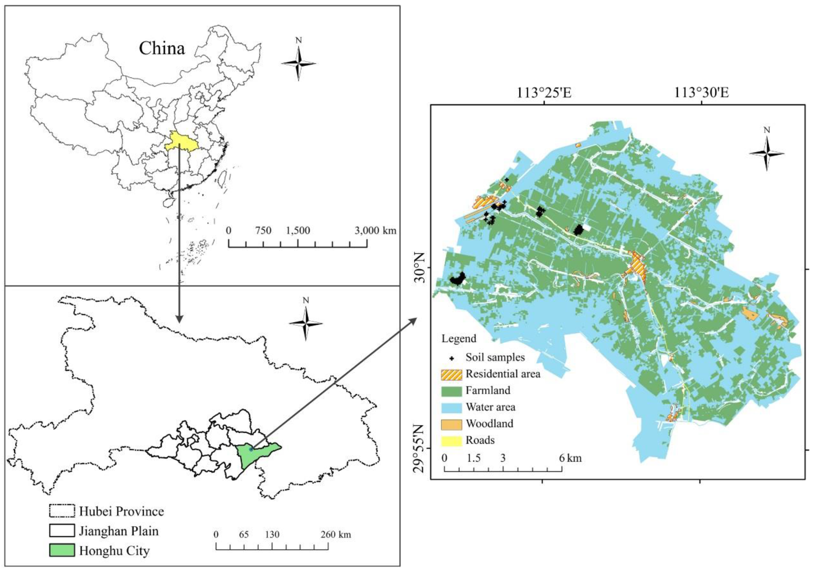
2.1. Study Area and Field Sampling

The area chosen for SOM estimation is called Honghu City, located in the east of Jianghan plain, Hubei Province (China) (Figure 1). It has a subtropical humid monsoon climate, with mean annual temperature and precipitation of approximately 16.1 °C and 1154 mm, respectively. This study area is one of the most crucial food production areas in Hubei Province, and its landform is characterized by plain, with mean elevation of below 50 m. In recent years, human activities have important influences on soil ecological environment.
The field sampling was conducted in December 2011 in an area of 29°59′30′′N to 30°2′30′′N and 113°22′0′′E to 113°26′30′′E. After removing stones, roots, plant residues and other large debris, 91 soil samples were collected from the topsoil (0–15 cm) and the geographical distributions of sampling points (recorded with a handy global positioning system) are shown in Figure 1. All the fresh samples were collected in labeled plastic bags. Soil water content of each soil sample was measured with a FieldScout TDR 300 (Spectrum Technologies Inc., Aurora, IL, USA). The land uses of these collected soil samples include artificial forest, pond, canal, meadow and irrigated cropland. According to USDA soil taxonomy, the soil type mainly belongs to Inceptisols. More detailed information on area and field sampling could be found in Liu et al. [33].

2.2. Spectral Measurement and Pre-Processing

Because the field spectral reflectance is sensitive to interference with the atmospheric water absorption [34], reflectance spectra of these 91 fresh soil samples were acquired in the laboratory. An ASD FieldSpec 3 spectrometer with a spectral range of 350–2500 nm was applied to measure the soil VIS–NIR spectra. This spectrometer had spectral resolutions of 3 nm between 350 and 1000 nm and 10 nm between 1000 and 2500 nm, but the output spectral resolution is automatically interpolated to 1 nm. For the spectral measurement, the soil samples were placed in petri dishes and labeled. The geometry parameters of the spectrometer were illustrated as follows: one external 50 W halogen light matched with the spectrometer was placed 30 cm away from the sample, with a 45° incidence angle; the sensor was positioned vertically and 12 cm above the sample surface. At the beginning of the spectral measurements and after every ten soil samples, the spectrometer was calibrated and optimized using a white Spectralon® panel [35]. Ten scans were obtained for each soil sample, and then averaged to one spectrum as the final reflectance spectra. All measurements were performed in a dark room to minimize the influence of external light. The fresh soil samples were denoted as moist samples, and their reflectance spectra were denoted as moist spectra.
The collected moist samples were then air-dried, gently ground and sieved to pass through 2 mm. The VIS–NIR spectra of the air-dried ground samples, denoted here as dried ground spectra, were measured following the same procedure as for moist samples.
The original spectral data was first narrowed to 400–2400 nm, and then Savitzky–Golay smoothing with 11 filter widths and a second-order polynomial was used to reduce the influences from the measuring instrument and spectral noises [36]. Then the spectra were resampled to 10 nm intervals to simplify the spectral matrix. Thus, a total of 201 wavebands ranging from 400 to 2400 nm were obtained for the subsequent analysis. In addition, continuum removal (CR) was used to extract useful information from reflectance spectra [37].

2.3. Chemical Analysis

The SOM contents of these dried ground samples were determined by wet oxidation at 180 °C with a mixture of potassium dichromate and sulfuric acid [33].

2.4. Fractional Order Derivative (FOD)

FOD extends the concept of integer order derivatives, and is a field devoting to the study of the properties and applications of arbitrary order derivative [14,15]. FOD method has been successfully used in system modeling, signal filtering and pattern recognition. There are three main types of FOD algorithm: Riemann–Liouville (R-L), Grünwald–Letnikov (G-L), and Caputo [38]. Among them, the definition of G-L is relatively simple, and was applied in our research.
Generally, the first derivative of function f(x) is defined as:
f ( x ) = lim h 0 f ( x + h ) f ( x ) h
where h is the increment of the independent variable x. Then the second derivative of function f(x) can be defined as:
f ( x ) = lim h 0 f ( x + h ) f ( x ) h = lim h 0 f ( x + 2 h ) 2 f ( x + h ) + f ( x ) h 2
If the derivative order of the function f(x) is increased to the higher order (v), and then the vth derivative order of the function f(x) can be expressed as:
f ( v ) ( x ) = lim h 0 1 h v m = 0 v ( 1 ) m ( v m ) f ( x m h )
Substituting the Gamma function into the binomial coefficient of Equation (3) and the fractional order is also simultaneously extended to the non-integer order, then we can obtain the v-order fractional derivative formula in the interval of [a, b] (G-L):
d v f ( x ) = lim h 0 1 h v m = 0 [ ( b a ) / h ] ( 1 ) m Γ ( v + 1 ) m ! Γ ( v m + 1 ) f ( x m h )
where h is the step length and is set to 1, and [(ba)/h] is the integer part of (ba)/h. The Gamma function is characterized by:
Γ ( z ) = 0 exp ( u ) u z 1 d u = ( z 1 ) !
Then Equation (4) can be converted to:
d v f ( x ) d x v f ( x ) + ( v ) f ( x 1 ) + ( v ) ( v + 1 ) 2 f ( x 2 ) + Γ ( v + 1 ) m ! Γ ( v + m + 1 ) f ( x m )
We applied Equation (6) to develop the FOD spectra using a program in Matlab R2014a (The MathWorks Inc.: Natick, MA, USA). In this study, v was allowed to vary from 0 to 2 (increment by 0.25 at each step). In particular, v = 0 indicated that the spectral data was not processed (i.e., the original reflectance spectra).

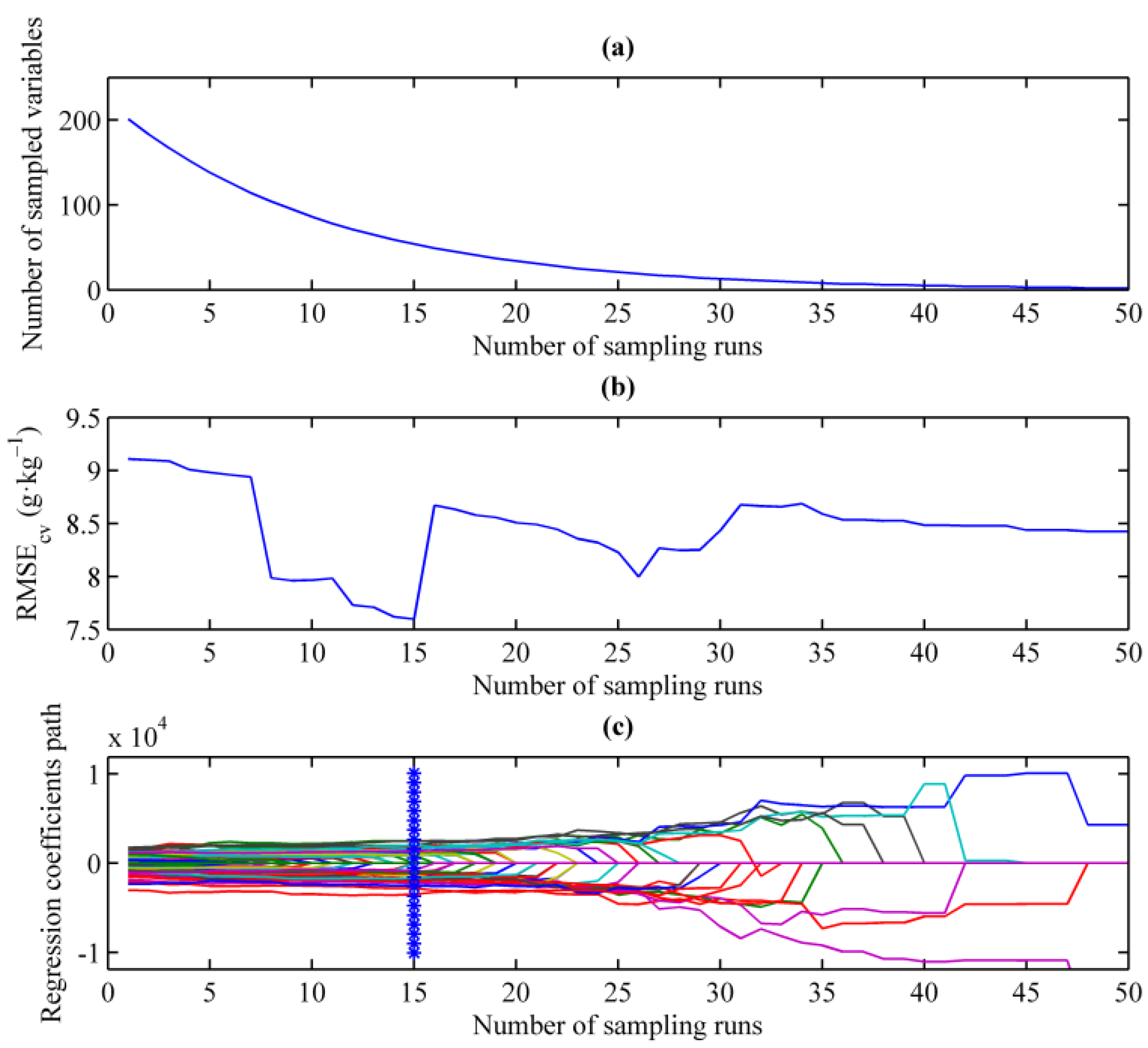
2.5. Spectral Variable Selection Techniques

Three spectral variable selection techniques were used to extract informative spectral variables, including CARS, ENET and GA. CARS method is an advanced variable selection technique proposed by Li et al. [22]. It imitates the principle of “survival of the fittest” from Darwin’s Biological Evolution Theory, aiming at selecting some key spectral variables with a computationally efficient procedure. According to the importance of each spectral variable (i.e., the absolute values of regression coefficients derived from PLS models), CARS selects N wavelength variable subsets from N Monte Carlo (MC) sampling runs in an iterative and competitive manner. In each run, CARS utilizes exponentially decreasing function (EDF) and adaptive reweighted sampling (ARS) to optimize the optimal spectral variable subset, together with the lowest root mean square error of cross validation (RMSEcv). A detailed description of this algorithm was given in Li et al. [22] and Vohland et al. [25]. The procedure of CARS was carried out in Matlab R2014a with lib PLS toolbox [22].
ENET is a sparse regression method based on the regularization of regression coefficients [27]. ENET shrinks the coefficients of redundant spectral variables to zero, by combining L1-norm penalty (lasso) and L2-norm penalty (ridge) together [27,28], and then the nonzero spectral variables were considered as effective wavelength variables. Compared with PLS with regression coefficient, elastic net with regression coefficient (named ENET) is more stable and reliable. Moreover, this method is not easy to overfit because of the removal of redundant and noisy variables. The whole process of the ENET method was conducted in Matlab R2014a with Glmnet toolbox available at http://web.stanford.edu/~hastie/glmnet_matlab/download.html (accessed on 19 September 2017).
GA variable selection is a method that can identify a subset of useful spectral variables while ensuring sufficient model accuracy [17,20,39,40]. It is a global optimization searching method, following “survival of the fittest” principle. Specific details of the entire process contain: (1) generating random variable subsets; (2) evaluating each individual subset for fitness to predict SOM; (3) discarding worse half of individuals; (4) breeding remaining individuals; (5) allowing for mutation. Loop to step 2 until the ending criteria are met. The root mean square error of cross validation (RMSEcv) was used for controlling the evolution (i.e., determining the optimal spectral variable subset). The following describes the parameter settings applied in our study: population size = 64, penalty slope = 0, window width = 1, mutation rate = 0.005, max generations = 100 and replicate runs = 10. GA procedure was performed in Matlab R2014a using the PLS Toolbox version 8.0.2 (Eigenvector Research, Inc., Wenatchee, WA, USA).

2.6. Model Calibration and Validation

The 91 soil samples were first ranked in ascending order based on SOM contents, then they were separated into 31 strata, and for each stratum (mostly 3 samples), one sample was selected as validation dataset (selecting the middle one, a total of 31 soil samples) and the remaining samples served as calibration dataset (a total of 60 soil samples).
SVM is a kernel-based learning method that is extensively employed for pattern classification and model regression, belonging to the nonlinear modeling technique [41,42]. In the modeling process, SVM algorithm maps original input data into a high-dimensional feature space through a kernel function [43]. It is able to deal with large input spaces efficiently [10,44]. For more details about SVM, readers are directed to Vapnik [41]. We used epsilon-SVM algorithm and radial basis function (RBF) to develop models. To calibrate epsilon-SVM, there are two parameters that need to be optimized: cost parameter C and RBF kernel parameter γ. A grid search technique with 5-fold cross-validation was used to optimize the combination of (C, γ). The optimal parameter was selected based on the smallest root mean square error of cross validation (RMSEcv). The SVM model was conducted in Matlab R2014a using the PLS Toolbox version 8.0.2.
Three statistical parameters were applied to evaluate the predictive abilities of the estimated models in the courses of cross-validation and validation: the coefficient of determination (R2), root mean squared error (RMSE) and ratio of the performance to deviation (RPD) [35]. Interpretations of RPD values were classified into five classes: RPD ≥ 2.5 (excellent models/predictions); 2.0 ≤ RPD < 2.5 (very good models/predictions); 1.8 ≤ RPD <2.0 (good models/predictions); 1.4 ≤ RPD < 1.8 (fair models/predictions); RPD < 1.4 (unsuccessful models/predictions). The optimum model should have the largest R2, RPD and the smallest RMSE.

3. Results

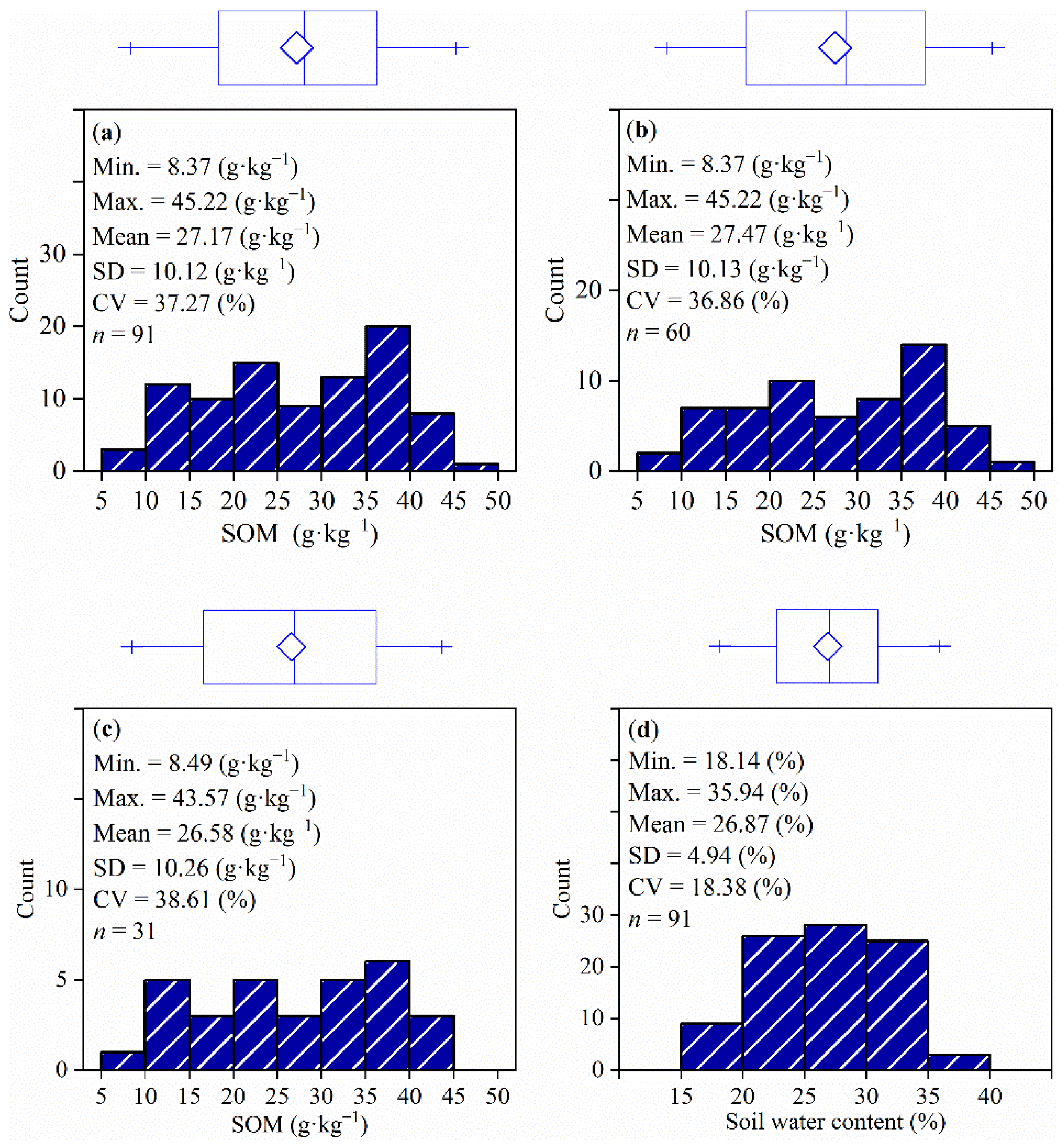
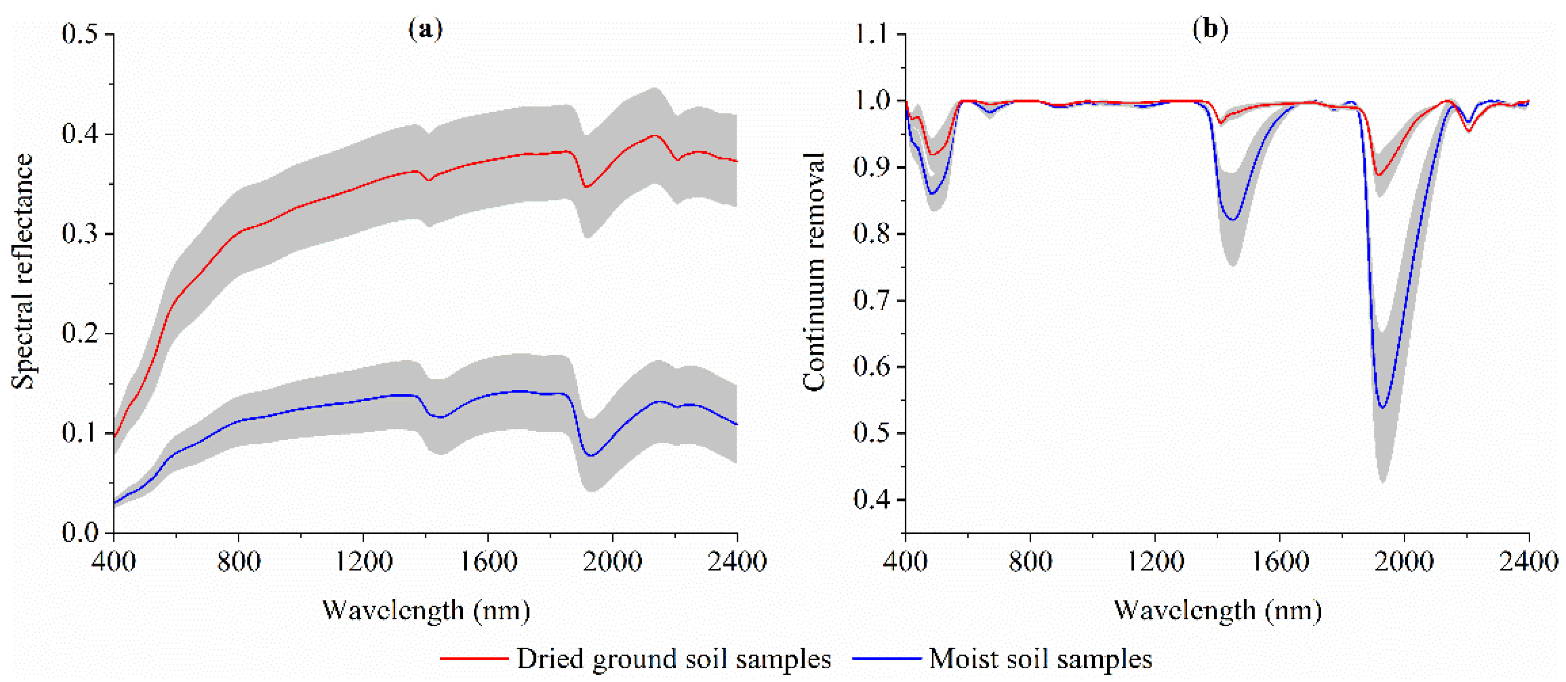
3.1. SOM, Soil Water Content and VIS–NIR Spectra
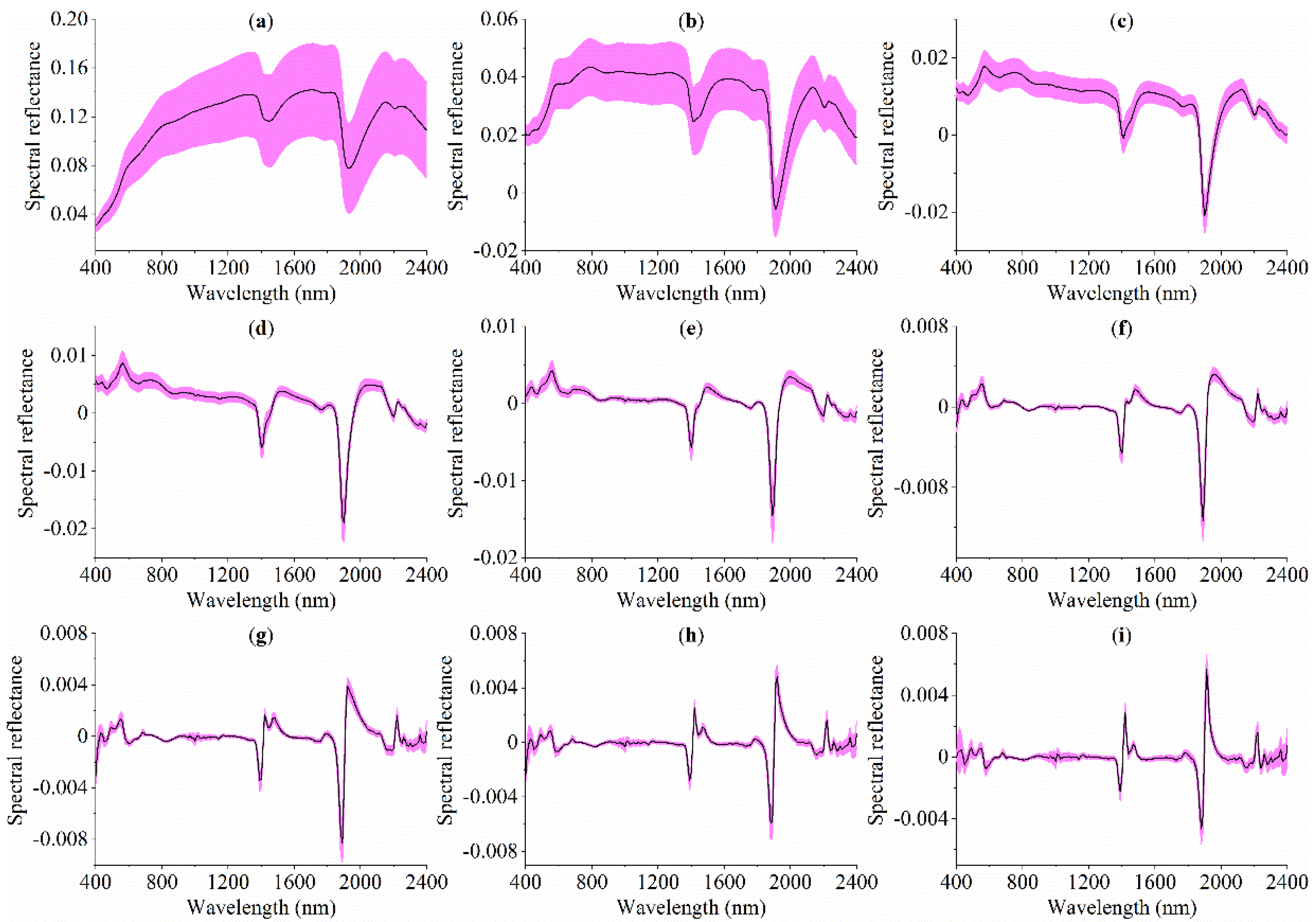
Statistical descriptions of measured SOM for the whole, calibration and validation dataset are shown in Figure 2. It could be observed that the whole dataset exhibited wide variation, with minimum, maximum and coefficient of variation (CV) of 8.37 g·kg−1, 45.22 g·kg−1 and 37.27%, respectively, which meant that the soil samples in the study area were diverse. Overall, the range of SOM contents observed in the validation dataset was well within the range of SOM contents in calibration dataset. The values of the mean, standard deviation (SD) and CV from these three datasets were relatively similar. Thus, the calibration dataset and the validation dataset can be considered representative of the whole population.
A summary of soil water content for the whole dataset is also provided in Figure 2. The soil water content varied between 18.14% and 35.94% with the mean and CV values of 26.87% and 18.38%, respectively.
To better analyze the influence of external environmental factors on moist samples (primarily from soil water), we compared the moist spectra with the dried ground spectra. Figure 3 shows the averaged reflectance spectra and averaged continuum removal spectra from dried ground and moist samples, respectively. The overall reflectance of the moist soils was lower than that of the dried ground soils (Figure 3a). Both dried ground spectra and moist spectra exhibited three obvious absorption features around 1450, 1950 and 2200 nm (Figure 3a). However, the spectral wavebands were broad and overlap, it was difficult to interpret. After performing the continuum removal (Figure 3b), the most prominent differences between the dried ground spectra and the moist spectra were mainly located within 400–580, 1340–1650 and 1850–2150 nm. The differences in the area of 400–580 nm were probably because of the interactions between soil color and soil water, and the differences in the 1340–1650 and 1850–2150 nm were mainly related to water absorption regions. In addition, compared with the dried ground spectra, the moist spectra had larger widths and depths at these wavelength regions. Overall, the differences between both were not linear across the entire spectrum.

3.2. FOD Spectra

Figure 4 shows a set of derivative spectra for the moist samples obtained from FOD (at different ν values). The original spectra in Figure 4a consist of three prominent absorption peaks near 1450, 1950 and 2200 nm, and over the visible range (400–780 nm), the reflectance spectra showed an increasing pattern. With the derivative order increasing, three prominent absorption peaks around 1450, 1950 and 2200 nm were gradually strengthened, and most reflectance values were progressively close to zero, evidencing that the overlapping peaks and baseline drifts were removed. Taking the absorption peak around 1950 nm as an example, its absorption feature was smoothly transformed to a bipolar shape at v = 2 (one positive peak and one negative peak). These detailed changes occurring in the spectral shape demonstrate the ability of FOD to interpolate between the integer order derivatives.
However, as the derivative order increased (v), the strength of the reflectance spectra decreased, noting the ordinate scales from Figure 4a–i. Besides, as v increased from 1 to 2, many small peaks appeared which indicated that the higher order derivative spectra were more susceptible to the interference of spectral noises. Simultaneously, higher order derivatives were better at isolating specific wavelengths.

3.3. Full-Spectrum SVM Models

SVM models for SOM estimation using full-spectrum (400–2400 nm) were established for different derivative orders (varying from 0 to 2), and the results of a series of calculations are given in Table 1. The nine SVM models provided different modeling results. All FOD transformations improved the model accuracies compared to the original reflectance (order = 0), because all these methods had the ability of reducing the adverse effects (e.g., baseline effects) and thus improved the model performance. The most accurate estimation was achieved by SVM model based on 1.5-order derivative spectra, with R2pre = 0.79, RMSEpre = 4.67 g·kg−1 and RPD = 2.20, then followed by 1.25-order derivative spectra. For the 1-order derivative spectra and 2-order derivative spectra, their RPD values reduced by 0.44 and 0.34, respectively, compared with 1.5-order derivative spectra, and their prediction accuracies could be classified as fair prediction and good prediction, respectively. Thus, it could manifest that, compared with the original reflectance (order = 0) and integer order derivatives (i.e., 1-order and 2-order), FOD at specific derivative orders could improve the model performance.

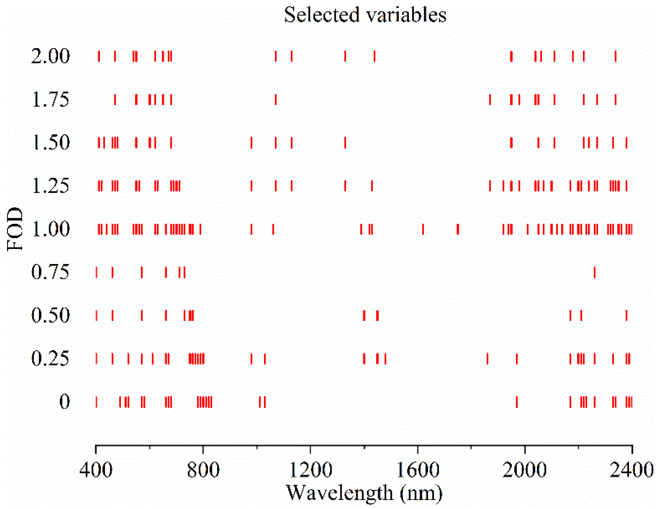
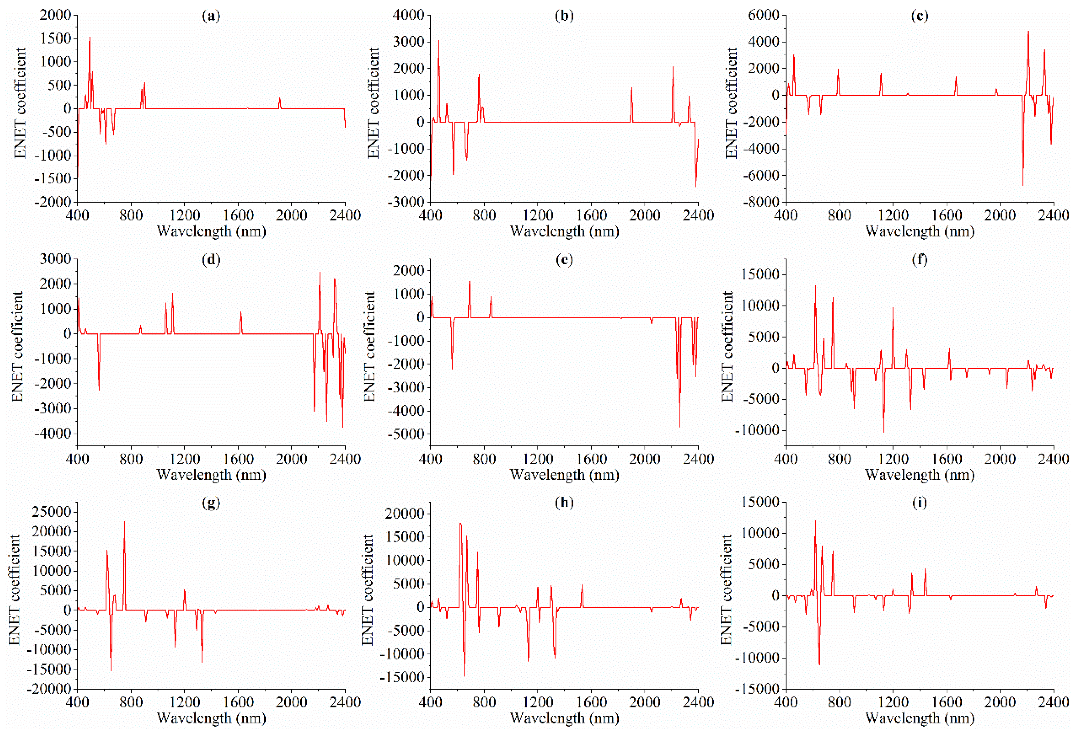
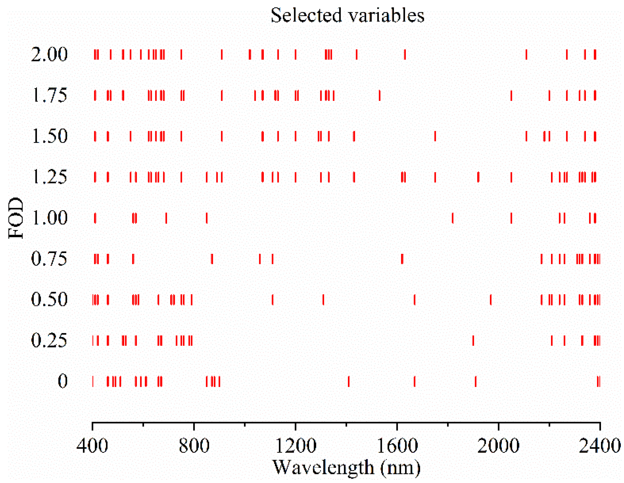
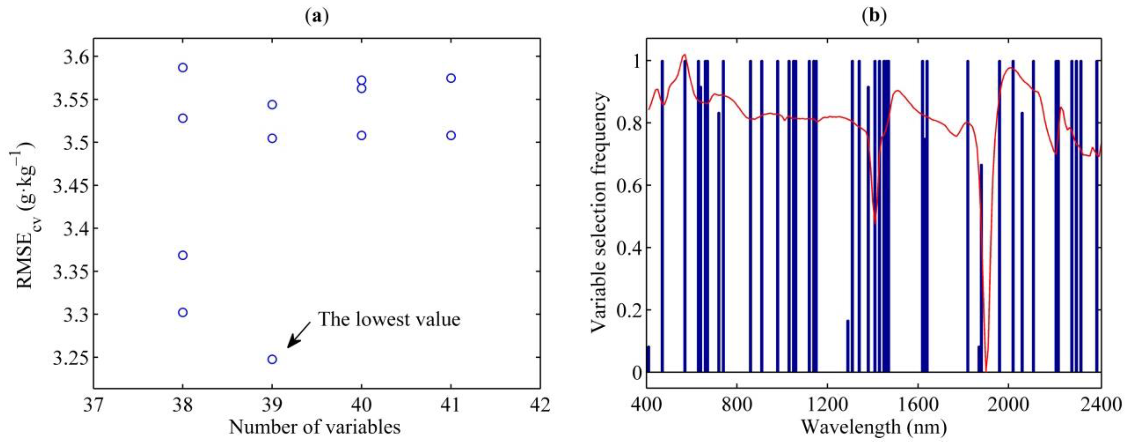
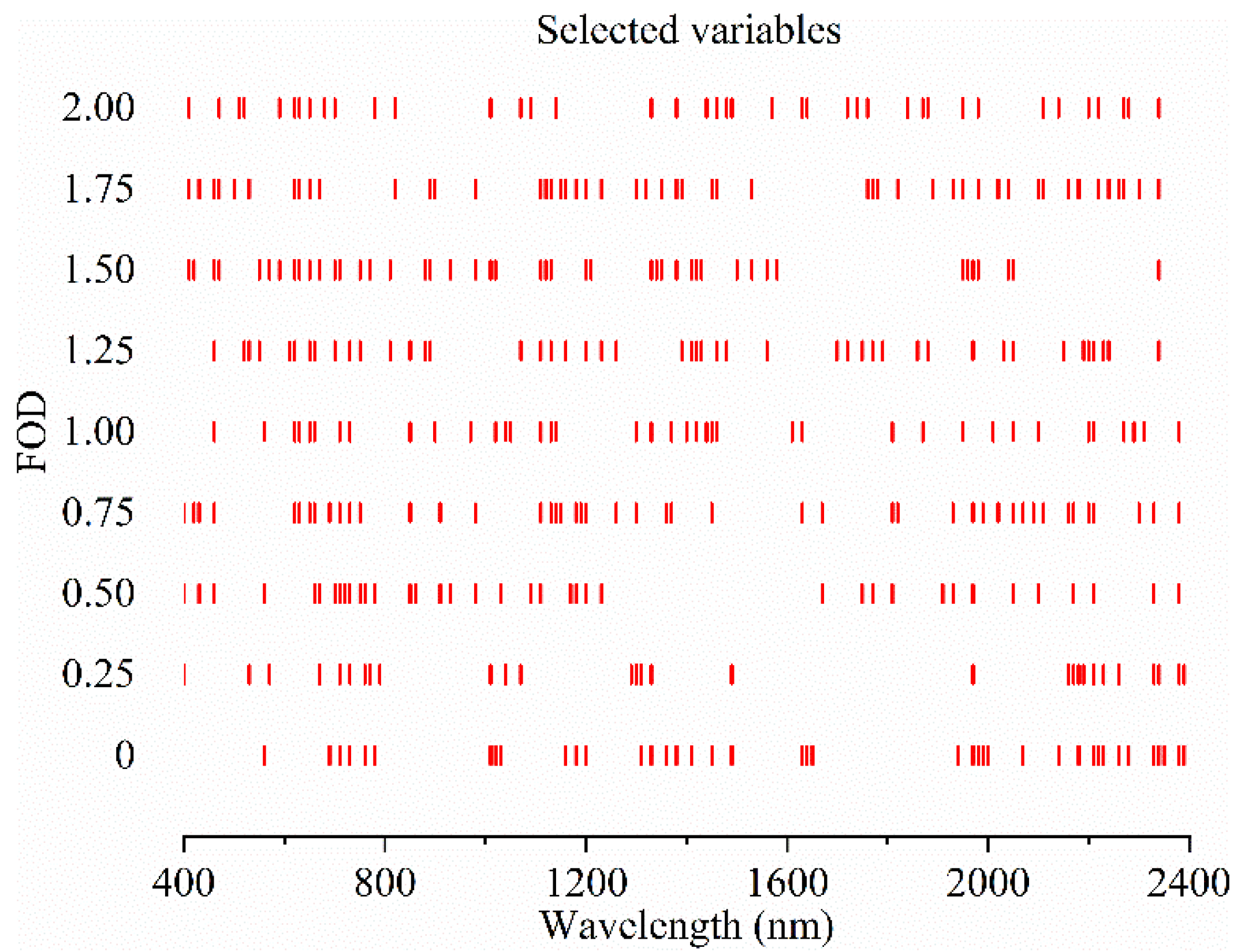
3.4. Spectral Variables Selected by CARS, ENET and GA

Taking the 1-order derivative spectra as an example, Figure 5a shows that with increasing number of sampling runs, the number of sampled spectral variables decreased, and the downward trend was from fast to slow. Figure 5b shows the change of RMSEcv values as the number of sampling runs increased. The smallest RMSEcv value was obtained when the number of sampling runs was equal to 15. The number of sampling runs less than 15 or more than 15 meant the elimination of uninformative variables and the loss of informational variables, respectively. Figure 5c illustrates the change in regression coefficient path for each variable during sampling. Together with Figure 5b, the optimal subset selected by the CARS method corresponded to the lowest RMSEcv value where it was marked by a vertical line of asterisk. Fifty-four spectral wavelength variables were retained as the most informative subset, which was just 26.87% of the number of the full-spectrum. The final selected spectral variables for all FOD transformations are illustrated in Figure 6.
The regression coefficients of ENET models for all FOD transformations are provided in Figure 7. After shrinking the regression coefficients of the redundant spectral variables to zero, the coefficients of ENET models were sparse over the entire spectral range. The final selected spectral variables for all FOD transformations are illustrated in Figure 8. When the derivative order was less than 1, the number of selected spectral variables was relatively small, whereas when derivative order was greater than 1, more spectral variables were selected and spread over the entire spectral range. Some relevant wavelengths were always selected in all FOD transformations, including wavelengths around 410, 460, 560, 2260 and 2390 nm.
For GA, the optimal spectral variable subset was selected according to the RMSEcv value, applied as a fitness function in GA variable selection. Taking the 1-order derivative spectra as an example, Figure 9a shows that when a subset of 39 spectral variables was selected, RMSEcv obtained the lowest value of 3.25 g·kg–1. Figure 9b shows the frequencies of 39 spectral variables occurring in the modeling process, with the selected wavelengths accounting for 19.40% of the full-spectrum. The final selected spectral variables for all FOD transformations are illustrated in Figure 10.

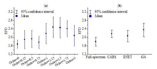
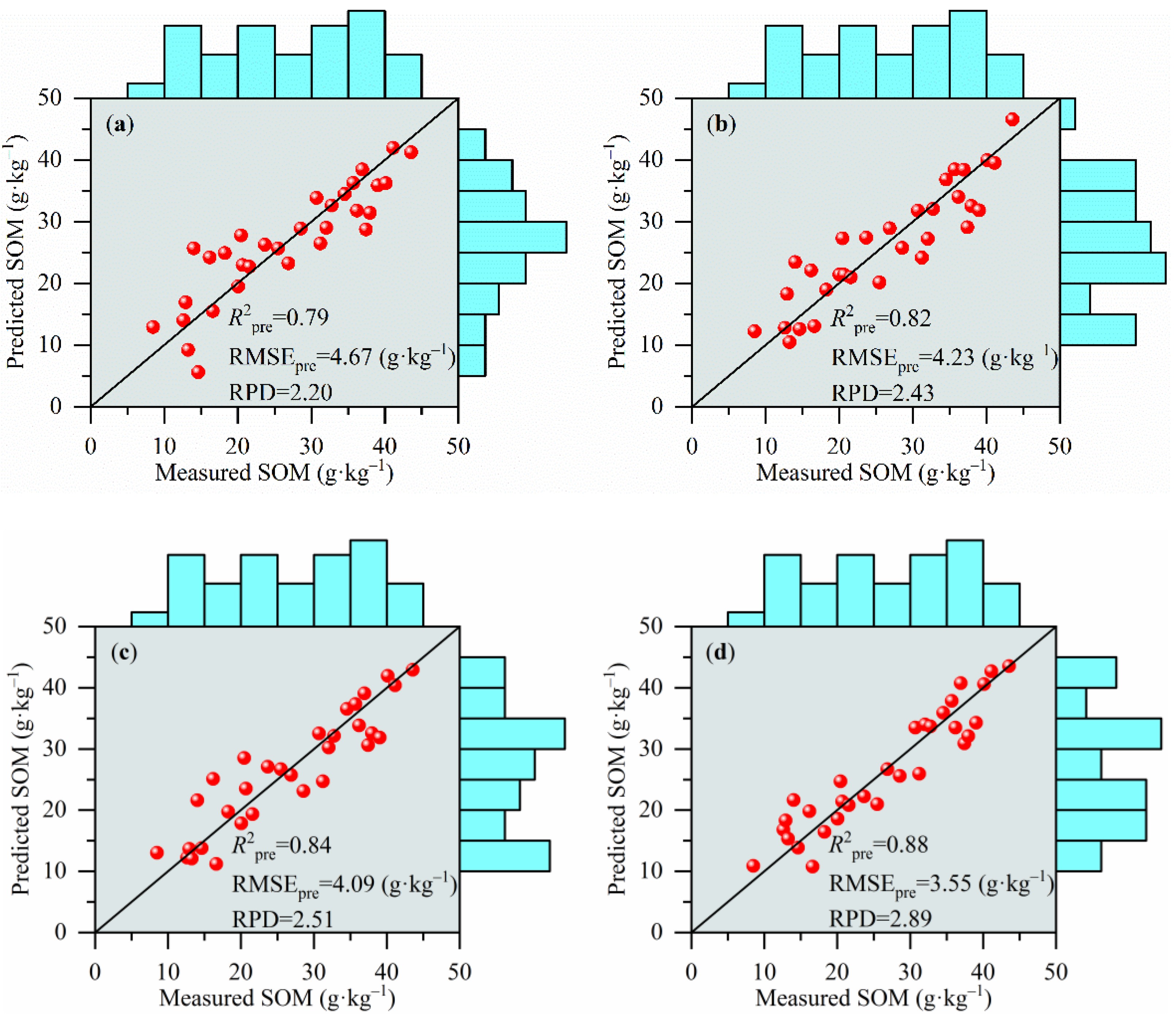
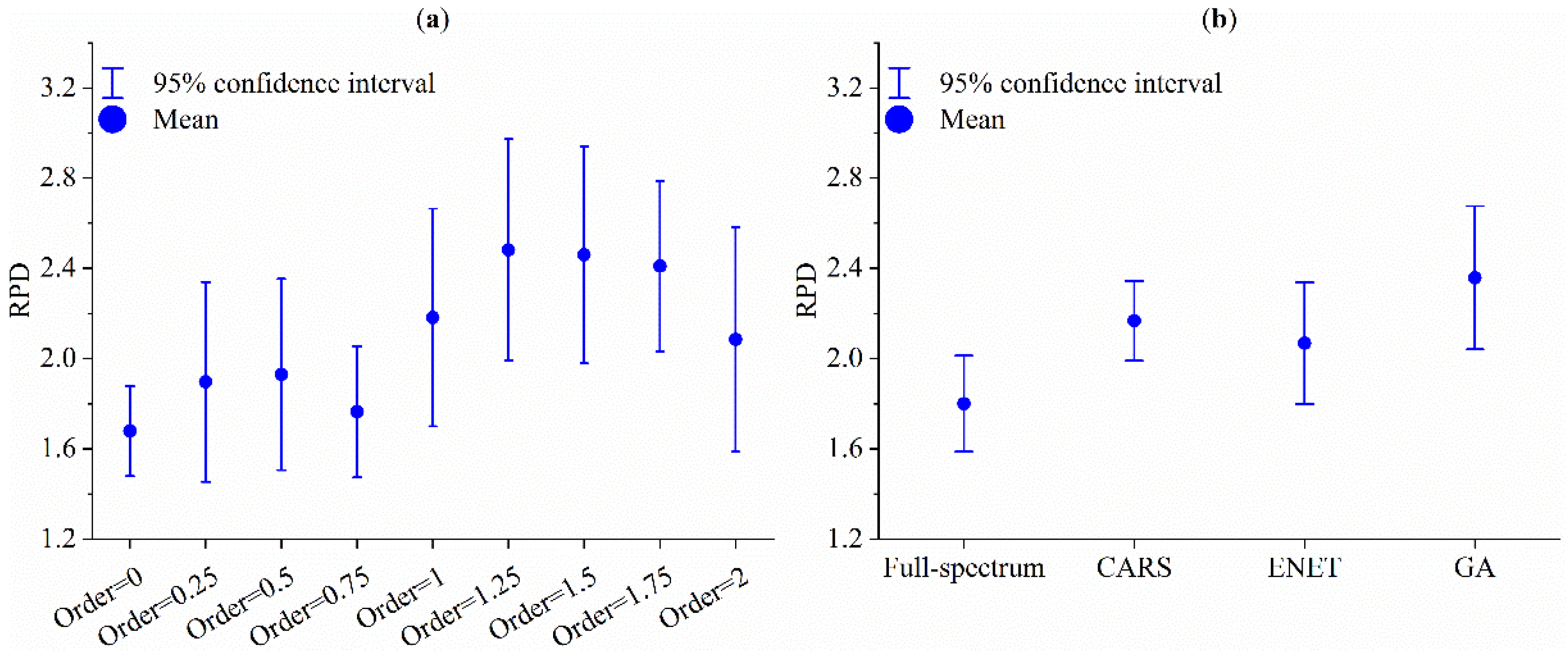
3.5. Comparison of Predictions Using Different FOD Transformations and Variable Selection Techniques

To investigate the influence of FOD and variable selection techniques on the estimation of SOM, spectroscopic models were built using SVM method with the same calibration dataset and validation dataset to make comparisons (but with different selected spectral wavelengths). The model accuracies were evaluated by R2, RMSE and RPD, and the descriptive regression statistics are shown in Table 2. Model cross-validation results demonstrated that after selecting the spectral variables, the simplified models showed better performance with higher values of R2cv (ranging from 0.66 to 0.96) and lower RMSEcv values (ranging from 1.94 g·kg–1 to 5.85 g·kg–1) than their corresponding full-spectrum SVM models (Table 1) for SOM estimation. Besides, the number of the selected spectral variables was greatly reduced (the simplifying ratios varied from 3.48% to 26.87%), and the selected spectral variables included the most useful information associated with SOM. In general, GA selected more spectral variables than CARS and ENET. These results indicate that the variable selection produce more effective models with simplified model structure and improved the model’s calibration performance.
Similar to the model accuracies in cross-validation, the validation dataset also provided better performances than those of the full-spectrum SVM models (Table 1), although the prediction accuracies of these models were inferior to the cross-validation. In CARS method, SVM model based on 1.25-order derivative spectra generated the highest predictive accuracy for SOM estimation (R2pre = 0.82, RMSEpre = 4.22 g·kg–1 and RPD = 2.43). The modeling results exhibited very good prediction. Likewise, SVM models based on 1.25-order derivative spectra and 1.5-order derivative spectra produced the most accurate estimation for SOM in ENET method and GA method, respectively. It should be noted that CARS, ENET and GA algorithms are positive in establishing more accurate and concise VIS–NIR models when compared to the full-spectrum SVM models (Table 1).
Figure 11 shows the scatter plots between the observed and predicted values of SOM from the optimal models with different variable selection methods. The measured vs. predicted SOM using the combination of 1.5-order derivative spectra and GA method more closely approached the 1:1 line (Figure 11d). In contrast, SOM prediction deviated from the 1:1 line in the SVM model based on full-spectrum of 1.5-order derivative spectra (Figure 11a).
When comparing the mean values of RPD for different FOD transformations (Figure 12a), SVM model based on 1.25-order derivative spectra achieved the best performance in all FOD transformations, with the mean RPD of 2.48, which exhibited a good potential of this preprocessing in spectral derivative in SOM estimation. The mean value of RPD for each variable selection technique is shown in Figure 12b. Regarding the results, GA presented the best performance, followed by CARS method and ENET method.
The optimal modeling method is generally the one that has the best predictive ability with a satisfactory accuracy. However, the choice of variable selection method is a compromise between the prediction performance and the computation time. The time to process each variable selection technique in Matlab R2014a was also calculated to further compare these algorithms (Table 2). All the procedures ran on the same computer with a 3.00 GHz Intel Core i5 processor, 8.00 GB RAM, and Windows 10 Professional Edition operating system. CARS and ENET were implemented within 1 s in all FOD transformations, but GA always consumed more than 100 s. The evaluation of the consumed time showed that CARS was the most efficient method, although its predictive performance was lower than GA (Figure 12b).

4. Discussion

Although VIS–NIR spectral techniques for SOM estimation using laboratory dried ground spectra are relatively well established [45,46], a lot of time and labor would be saved if the moist spectra can be applied to estimate SOM with acceptable performance. Our results demonstrated that moist spectra and dried ground spectra differed greatly from each other (Figure 3a). This corresponded well with other studies: with increasing soil water content, reflectance spectra decreased over the entire wavelength range [4,9,47,48,49,50,51]. This is mainly because soil water replaces the air within the micro and macro pores, leading to increasing the forward scattering of light and increasing the absorption at all wavelengths [52]. In addition, other external factors also affect the spectral characteristics of moist soil, including the condition of the soil surface, sample preparation and the particle size [4,45,46,53]. Despite the negative effects of moisture on soil spectra, good prediction performance was obtained with the different modeling techniques in this study (the best validation RPD = 2.89). Overall, our results show that there is great potential in using the moist spectra to estimate SOM, and the optimal model accuracy was comparable to those reported from studies. Li et al. [9] applied least-squares support vector machine to predict SOC of field samples, and their validation result was slightly lower (R2 = 0.81). In Yujiang County of Central China, a study presented by Xu et al. [18] indicated that SVM achieved the best performance for SOM estimation with validation RPD of 2.84.
The application of the derivative method in VIS–NIR spectra is able to eliminate background noises, sharpen spectral features, improve the spectral resolution of overlapped peaks and extract important spectral information [13,54,55]. Generally, 1-order derivative stands for the slope of the reflectance spectra, and 2-order derivative stands for the curvature of the reflectance spectra [56]. Nonetheless, although 1-order derivative and 2-order derivative can increase the spectral difference, a very large difference still exists between the original spectral curve and 1-order derivative/2-order derivative, which may result to the omission of useful information. A major advantage of FOD is that it permits flattening of baselines with a wide range of curvatures [54]. Thus, similar to the integer order derivatives, FOD can eliminate sloping baselines, but its ability is proved to be better than that of integer order derivatives, as it allows elimination baselines with different degrees of curvature. In all full-spectrum SVM models (Table 1), SVM model based on 1.5-order derivative spectra provided the greatest accuracy, with validation RPD = 2.20. In comparison with 1-order derivative spectra, 2-order derivative spectra and the original spectral reflectance, its RPD improved by 0.44, 0.34 and 0.68, respectively.
Many studies demonstrated that in most cases, the modeling results using 1-order derivative spectra showed better predictive abilities than the 2-order derivative spectra in predicting soil properties. For example, Nawar et al. [10] reported that 1-order derivative spectra presented better calibration performances than 2-order derivative spectra for SOM estimation, regardless of the partial least squares, SVM and multivariate adaptive regression splines applied. Srivastava et al. [57] reported relatively poorer prediction result for monitoring of soil organic carbon in the Indo-Gangetic Plains of Punjab, India when using 2-order derivative spectra, as compared with that of 1-order derivative spectra. Similar to their results, our study also found the same pattern (Table 1 and Table 2).
Soil VIS–NIR spectra often contain redundant wavelength information and can increase the model complexity [23,24,58,59]. It could be observed that the SVM models based on the selected spectral variables yielded superior model performance relative to the full-spectrum SVM models for SOM, regardless of FOD transformations (Table 1 and Table 2 and Figure 12b). The RPD of the optimal model was 2.89, while for full-spectrum SVM model of 0-order derivative spectra (i.e., without using any variable selection techniques), the RPD was 1.52. The improvement of the optimal model can be ascribed to the result that it excludes the unnecessary spectral variables to decrease model over-fitting, implying that variable selection can simplify the model structure and improve the model robustness [60,61].
Among the three spectral variable selection methods that were applied, GA method exhibited the highest predictive performance in all FOD transformations (Figure 12). These models were classified as fair predictions to excellent predictions, with validation RPD values ranging from 1.74 to 2.89. CARS method presented relatively inferior model results compared to the GA method, and the poorest result was achieved by ENET (Figure 12b, only concerning the mean values). Nonetheless, GA consumed the longest amount of computation time (the mean value = 119.71 s) and was complex to conduct an exhaustive search for the possible combinations. As an alternative, CARS method was recommended instead of GA method for its accuracy and the computational efficiency. Some previous studies also showed that CARS is a potential tool in selecting useful spectral variables, for instance, Vohland et al. [25] and Xu et al. [26]. The application of ENET did not produce satisfactory results (Table 2 and Figure 12). Although the number of selected spectral variables was much reduced and the model structure was also simplified, the models built on ENET selected variables were relatively worse in terms of lower R2 and RPD and larger RMSE. This may be due to the fact that the ENET method only reflects the importance of spectral variables, but this method is not suitable for selecting the optimal subset of spectral variables, since the combination of the selected spectral variables can significantly affect model performance. However, the results with ENET were still better than the FOD with full-spectrum alone (except 2-order derivative spectra).
In general, GA method generated sparser distributions of useful spectral variables over the entire wavelength range than CARS and ENET methods. The main reason is that this method is a kind of global optimization searching method inspired by natural selection mechanisms. Spectral variables are selected collectively with considering joint efforts (i.e., considering the interaction of variables), and this method has a stochastic nature [17,23]. When using GA method to select useful spectral variables, other studies also reported similar phenomena, such as Pang et al. [62], Xu et al. [26], Shi et al. [32]. Some spectral variables were always selected by GA method across all FOD transformations (Figure 10), such as wavelengths around 560, 660, 710, 750, 1020, 1970, 2210 and 2340 nm, although some differences were observed (within 20 nm). The selected variables of approximately 660, 710, 750, 1020, 1970, 2210 and 2340 nm are featured by the presence of Fe oxides, O–H, N–H, C–OH and AL–OH [16]. The spectral variables selected by CARS in all FOD transformations were mainly grouped within 400–800 and 2000–2400 nm. For ENET method, wavelengths within 400–800 and 2200–2400 nm were always selected. These findings are in accordance with other studies [23,63], especially the bands in the visible region. However, we should note that the overall selection pattern may vary from one dataset to another.
SVM algorithm has been widely applied to solve the complicated regression problems. Recently, Dotto et al. [12] reviewed a series of the multivariate methods and investigated their influences on the SOC prediction. Their results indicated that SVM achieved the highest performance in the SOC estimation, among the nine commonly used multivariate methods. The results from our study support their findings. Our previous study has showed that soil water had a nonlinear effect on reflectance spectra [5]. The wavebands after variable selection would definitely reduce the spectral variables involved in modeling, but these processes cannot change the nonlinear relation between soil water and reflectance spectra. Thus, the application of SVM model is sufficiently flexible to solve these complex and non-linear regression problems. The reason for this can be attributed to two aspects: first, the epsilon-insensitive loss function applied in SVM model is robust to outliers. Second, through the “kernel trick”, SVM can be easily extended to the nonlinear-SVM [61].
The soil samples applied were mainly selected from the same soil type, so that these soil samples shared similar spectral characteristics and then could develop an exclusive prediction model. Although relatively accurate predictions for SOM in moist soil were obtained in this study, all estimation models had RPD values below 3, meaning that there is still possible potential for improvement of the predictive accuracy. However, the spectral preprocessing and chemometric modeling reported in this paper is a promising start, and we intend to validate these methods to diverse datasets that include various soil types, geographical origins, soil textures and clay minerals in future research. Remotely sensed spectral data are acquired using air- or space-borne sensors, which can allow rapid acquisition of large-scale spectral information of target objects, and a number of next-generation hyperspectral sensors are also planned to be launched in the next few years [64]. Therefore, the potentials of these sensors to estimate SOM should be explored in the future.

5. Conclusions

This study explored the effectiveness of the combinations of FOD and spectral variable selection methods for moist SOM estimation. The principal results indicated that:
(1)
The overall reflectance of moist spectra was lower than dried ground spectra. With increasing order of derivative, the overlapping peaks and baseline drifts were gradually removed, but the spectral strength decreased simultaneously.
(2)
In some cases, FOD (e.g., 1.25-order and 1.5-order) could generate better estimation than integer order derivatives (i.e., 1-order and 2-order) and original reflectance spectra.
(3)
The SVM model based on 1.5 derivative spectra and GA method provided the optimal model prediction, with validation RPD of 2.89. Our study confirms the potential of moist VIS–NIR spectra to estimate SOM.
(4)
Variable selection (i.e., CARS, ENET and GA) was able to select the useful spectral variables, and the simplified models showed the improved prediction accuracies. Overall, GA produced the best predictive result, but it also consumed long computation time. One alternative is to apply CARS method because it takes less time to process the algorithm without significantly reducing the model performance.

Acknowledgments

This research was financially supported by the National Natural Science Foundation of China (41771440 and 41501444).

Author Contributions

Yongsheng Hong, Yiyun Chen, Lei Yu and Yong Zhang conceived and designed the research. Yongsheng Hong performed all the modelling. Yi Liu and Hang Cheng performed the experiments. Yanfang Liu and Yaolin Liu participated in the data analyses. Yongsheng Hong and Yiyun Chen were involved in drafting and revising the manuscript.

Conflicts of Interest

The authors declare no conflict of interest.

References

  1. Schlesinger, W.H.; Andrews, J.A. Soil respiration and the global carbon cycle. Biogeochemistry 2000, 48, 7–20. [Google Scholar] [CrossRef]
  2. Lal, R. Soil carbon sequestration to mitigate climate change. Geoderma 2004, 123, 1–22. [Google Scholar] [CrossRef]
  3. Lobsey, C.R.; Viscarra Rossel, R.A.; Roudier, P.; Hedley, C.B. Rs-local data-mines information from spectral libraries to improve local calibrations. Eur. J. Soil Sci. 2017, 68, 840–852. [Google Scholar] [CrossRef]
  4. Kuhnel, A.; Bogner, C. In-situ prediction of soil organic carbon by VIS–NIR spectroscopy: An efficient use of limited field data. Eur. J. Soil Sci. 2017, 68, 689–702. [Google Scholar] [CrossRef]
  5. Hong, Y.S.; Yu, L.; Chen, Y.Y.; Liu, Y.F.; Liu, Y.L.; Liu, Y.; Cheng, H. Prediction of soil organic matter by VIS–NIR spectroscopy using normalized soil moisture index as a proxy of soil moisture. Remote Sens. 2018, 10, 28. [Google Scholar] [CrossRef]
  6. Ogen, Y.; Neumann, C.; Chabrillat, S.; Goldshleger, N.; Ben Dor, E. Evaluating the detection limit of organic matter using point and imaging spectroscopy. Geoderma 2018, 321, 100–109. [Google Scholar] [CrossRef]
  7. Mouazen, A.M.; Maleki, M.R.; De Baerdemaeker, J.; Ramon, H. On-line measurement of some selected soil properties using a VIS–NIR sensor. Soil Tillage Res. 2007, 93, 13–27. [Google Scholar] [CrossRef]
  8. Nocita, M.; Kooistra, L.; Bachmann, M.; Muller, A.; Powell, M.; Weel, S. Predictions of soil surface and topsoil organic carbon content through the use of laboratory and field spectroscopy in the Albany Thicket Biome of Eastern Cape Province of South Africa. Geoderma 2011, 167–168, 295–302. [Google Scholar] [CrossRef] [Green Version]
  9. Li, S.; Shi, Z.; Chen, S.C.; Ji, W.J.; Zhou, L.Q.; Yu, W.; Webster, R. In situ measurements of organic carbon in soil profiles using VIS–NIR spectroscopy on the Qinghai-Tibet plateau. Environ. Sci. Technol. 2015, 49, 4980–4987. [Google Scholar] [CrossRef] [PubMed]
  10. Nawar, S.; Buddenbaum, H.; Hill, J.; Kozak, J.; Mouazen, A.M. Estimating the soil clay content and organic matter by means of different calibration methods of VIS–NIR diffuse reflectance spectroscopy. Soil Tillage Res. 2016, 155, 510–522. [Google Scholar] [CrossRef]
  11. Rinnan, Å.; Berg, F.v.d.; Engelsen, S.B. Review of the most common pre-processing techniques for near-infrared spectra. TrAC Trend Anal. Chem. 2009, 28, 1201–1222. [Google Scholar]
  12. Dotto, A.C.; Dalmolin, R.S.D.; ten Caten, A.; Grunwald, S. A systematic study on the application of scatter-corrective and spectral-derivative preprocessing for multivariate prediction of soil organic carbon by VIS–NIR spectra. Geoderma 2018, 314, 262–274. [Google Scholar] [CrossRef]
  13. Tong, P.J.; Du, Y.P.; Zheng, K.Y.; Wu, T.; Wang, J.J. Improvement of NIR model by fractional order Savitzky-Golay derivation (FOSGD) coupled with wavelength selection. Chemom. Intell. Lab. 2015, 143, 40–48. [Google Scholar] [CrossRef]
  14. Li, Y.L.; Pan, C.; Meng, X.; Ding, Y.Q.; Chen, H.X. Haar wavelet based implementation method of the non-integer order differentiation and its application to signal enhancement. Meas. Sci. Rev. 2015, 15, 101–106. [Google Scholar] [CrossRef]
  15. Zhang, D.; Tiyip, T.; Ding, J.L.; Zhang, F.; Nurmemet, I.; Kelimu, A.; Wang, J.Z. Quantitative estimating salt content of saline soil using laboratory hyperspectral data treated by fractional derivative. J. Spectrosc. 2016, 2016, 1081674. [Google Scholar] [CrossRef]
  16. Viscarra Rossel, R.A.; Behrens, T. Using data mining to model and interpret soil diffuse reflectance spectra. Geoderma 2010, 158, 46–54. [Google Scholar] [CrossRef]
  17. Vohland, M.; Ludwig, M.; Thiele-Bruhn, S.; Ludwig, B. Quantification of soil properties with hyperspectral data: Selecting spectral variables with different methods to improve accuracies and analyze prediction mechanisms. Remote Sens. 2017, 9, 1103. [Google Scholar] [CrossRef]
  18. Xu, S.X.; Zhao, Y.C.; Wang, M.Y.; Shi, X.Z. Comparison of multivariate methods for estimating selected soil properties from intact soil cores of paddy fields by VIS–NIR spectroscopy. Geoderma 2018, 310, 29–43. [Google Scholar] [CrossRef]
  19. Chong, I.G.; Jun, C.H. Performance of some variable selection methods when multicollinearity is present. Chemom. Intell. Lab. 2005, 78, 103–112. [Google Scholar] [CrossRef]
  20. Jarvis, R.M.; Goodacre, R. Genetic algorithm optimization for pre-processing and variable selection of spectroscopic data. Bioinformatics 2005, 21, 860–868. [Google Scholar] [CrossRef] [PubMed]
  21. Galvão, R.K.H.; Araújo, M.C.U.; Fragoso, W.D.; Silva, E.C.; José, G.E.; Soares, S.F.C.; Paiva, H.M. A variable elimination method to improve the parsimony of MLR models using the successive projections algorithm. Chemom. Intell. Lab. 2008, 92, 83–91. [Google Scholar] [CrossRef]
  22. Li, H.D.; Liang, Y.Z.; Xu, Q.S.; Cao, D.S. Key wavelengths screening using competitive adaptive reweighted sampling method for multivariate calibration. Anal. Chim. Acta 2009, 648, 77–84. [Google Scholar] [CrossRef] [PubMed]
  23. Vohland, M.; Ludwig, M.; Harbich, M.; Emmerling, C.; Thiele-Bruhn, S. Using variable selection and wavelets to exploit the full potential of visible-near infrared spectra for predicting soil properties. J. Near Infrared Spec. 2016, 24, 255–269. [Google Scholar] [CrossRef]
  24. Vohland, M.; Harbich, M.; Ludwig, M.; Emmerling, C.; Thiele-Bruhn, S. Quantification of soil variables in a heterogeneous soil region with VIS–NIR–SWIR data using different statistical sampling and modeling strategies. IEEE J. Sel. Top. Appl. 2016, 9, 4011–4021. [Google Scholar] [CrossRef]
  25. Vohland, M.; Ludwig, M.; Thiele-Bruhn, S.; Ludwig, B. Determination of soil properties with visible to near- and mid-infrared spectroscopy: Effects of spectral variable selection. Geoderma 2014, 223, 88–96. [Google Scholar] [CrossRef]
  26. Xu, S.X.; Zhao, Y.C.; Wang, M.Y.; Shi, X.Z. Determination of rice root density from VIS–NIR spectroscopy by support vector machine regression and spectral variable selection techniques. Catena 2017, 157, 12–23. [Google Scholar] [CrossRef]
  27. Zou, H.; Hastie, T. Regularization and variable selection via the elastic net. J. R. Stat. Soc. B 2005, 67, 301–320. [Google Scholar] [CrossRef]
  28. Liu, W.Y.; Li, Q. An efficient elastic net with regression coefficients method for variable selection of spectrum data. PLoS ONE 2017, 12, e0171122. [Google Scholar] [CrossRef] [PubMed]
  29. Niazi, A.; Leardi, R. Genetic algorithms in chemometrics. J. Chemom. 2012, 26, 345–351. [Google Scholar] [CrossRef]
  30. Leardi, R.; Lupiáñez González, A. Genetic algorithms applied to feature selection in PLS regression: How and when to use them. Chemom. Intell. Lab. 1998, 41, 195–207. [Google Scholar] [CrossRef]
  31. Jiang, Q.H.; Liu, M.X.; Wang, J.; Liu, F. Feasibility of using visible and near-infrared reflectance spectroscopy to monitor heavy metal contaminants in urban lake sediment. Catena 2018, 162, 72–79. [Google Scholar] [CrossRef]
  32. Shi, T.Z.; Chen, Y.Y.; Liu, H.Z.; Wang, J.J.; Wu, G.F. Soil organic carbon content estimation with laboratory-based visible-near-infrared reflectance spectroscopy: Feature selection. Appl. Spectrosc. 2014, 68, 831–837. [Google Scholar] [CrossRef] [PubMed]
  33. Liu, Y.L.; Jiang, Q.H.; Fei, T.; Wang, J.J.; Shi, T.Z.; Guo, K.; Li, X.R.; Chen, Y.Y. Transferability of a visible and near-infrared model for soil organic matter estimation in riparian landscapes. Remote Sens. 2014, 6, 4305–4322. [Google Scholar] [CrossRef]
  34. Qi, H.J.; Paz-Kagan, T.; Karnieli, A.; Li, S.W. Linear multi-task learning for predicting soil properties using field spectroscopy. Remote Sens. 2017, 9, 1099. [Google Scholar] [CrossRef]
  35. Romero, D.J.; Ben-Dor, E.; Demattê, J.A.M.; Souza, A.B.E.; Vicente, L.E.; Tavares, T.R.; Martello, M.; Strabeli, T.F.; Barros, P.P.D.; Fiorio, P.R.; et al. Internal soil standard method for the Brazilian soil spectral library: Performance and proximate analysis. Geoderma 2018, 312, 95–103. [Google Scholar] [CrossRef]
  36. Savitzky, A.; Golay, M.J.E. Smoothing and differentiation of data by simplified least squares procedures. Anal. Chem. 1964, 36, 1627–1639. [Google Scholar] [CrossRef]
  37. Clark, R.N.; Roush, T.L. Reflectance spectroscopy—Quantitative-analysis techniques for remote-sensing applications. J. Geophys. Res. 1984, 89, 6329–6340. [Google Scholar] [CrossRef]
  38. Benkhettou, N.; da Cruz, A.; Torres, D.F.M. A fractional calculus on arbitrary time scales: Fractional differentiation and fractional integration. Signal Process. 2015, 107, 230–237. [Google Scholar] [CrossRef]
  39. Leardi, R.; Boggia, R.; Terrile, M. Genetic algorithms as a strategy for feature-selection. J. Chemometr. 1992, 6, 267–281. [Google Scholar] [CrossRef]
  40. Wang, J.J.; Cui, L.J.; Gao, W.X.; Shi, T.Z.; Chen, Y.Y.; Gao, Y. Prediction of low heavy metal concentrations in agricultural soils using visible and near-infrared reflectance spectroscopy. Geoderma 2014, 216, 1–9. [Google Scholar] [CrossRef]
  41. Vapnik, V.N. An overview of statistical learning theory. IEEE Trans. Neural Netw. 1999, 10, 988–999. [Google Scholar] [CrossRef] [PubMed]
  42. Chang, C.C.; Lin, C.J. LIBSVM: A library for support vector machines. ACM Trans. Intell. Syst. Technol. 2011, 2. [Google Scholar] [CrossRef]
  43. Thissen, U.; Pepers, M.; Ustun, B.; Melssen, W.J.; Buydens, L.M.C. Comparing support vector machines to PLS for spectral regression applications. Chemom. Intell. Lab. 2004, 73, 169–179. [Google Scholar] [CrossRef]
  44. Luca, F.; Conforti, M.; Castrignano, A.; Matteucci, G.; Buttafuoco, G. Effect of calibration set size on prediction at local scale of soil carbon by VIS–NIR spectroscopy. Geoderma 2017, 288, 175–183. [Google Scholar] [CrossRef]
  45. Franceschini, M.H.D.; Demattê, J.A.M.; Kooistra, L.; Bartholomeus, H.; Rizzo, R.; Fongaro, C.T.; Molin, J.P. Effects of external factors on soil reflectance measured on-the-go and assessment of potential spectral correction through orthogonalisation and standardisation procedures. Soil Tillage Res. 2018, 177, 19–36. [Google Scholar] [CrossRef]
  46. Ji, W.; Rossel, R.A.V.; Shi, Z. Accounting for the effects of water and the environment on proximally sensed VIS–NIR soil spectra and their calibrations. Eur. J. Soil Sci. 2015, 66, 555–565. [Google Scholar] [CrossRef]
  47. Ackerson, J.P.; Morgan, C.L.S.; Ge, Y. Penetrometer-mounted VIS–NIR spectroscopy: Application of EPO-PLS to in situ VIS–NIR spectra. Geoderma 2017, 286, 131–138. [Google Scholar] [CrossRef]
  48. Wijewardane, N.K.; Ge, Y.F.; Morgan, C.L.S. Moisture insensitive prediction of soil properties from VNIR reflectance spectra based on external parameter orthogonalization. Geoderma 2016, 267, 92–101. [Google Scholar] [CrossRef]
  49. Roudier, P.; Hedley, C.B.; Lobsey, C.R.; Rossel, R.A.V.; Leroux, C. Evaluation of two methods to eliminate the effect of water from soil VIS–NIR spectra for predictions of organic carbon. Geoderma 2017, 296, 98–107. [Google Scholar] [CrossRef]
  50. Minasny, B.; McBratney, A.B.; Bellon-Maurel, V.; Roger, J.M.; Gobrecht, A.; Ferrand, L.; Joalland, S. Removing the effect of soil moisture from NIR diffuse reflectance spectra for the prediction of soil organic carbon. Geoderma 2011, 167–168, 118–124. [Google Scholar] [CrossRef]
  51. Yu, L.; Hong, Y.S.; Zhu, Y.X.; Huang, P.; He, Q.; Qi, F. Removing the effect of soil moisture content on hyperspectral reflectance for the estimation of soil organic matter content. Spectrosc. Spectr. Anal. 2017, 37, 2146–2151. (In Chinese) [Google Scholar]
  52. Lobell, D.B.; Asner, G.P. Moisture effects on soil reflectance. Soil Sci. Soc. Am. J. 2002, 66, 722–727. [Google Scholar] [CrossRef]
  53. Terra, F.S.; Demattê, J.A.M.; Viscarra Rossel, R.A. Proximal spectral sensing in pedological assessments: VIS–NIR spectra for soil classification based on weathering and pedogenesis. Geoderma 2018, 318, 123–136. [Google Scholar] [CrossRef]
  54. Schmitt, J.M. Fractional derivative analysis of diffuse reflectance spectra. Appl. Spectrosc. 1998, 52, 840–846. [Google Scholar] [CrossRef]
  55. Wang, J.Z.; Tiyip, T.; Ding, J.L.; Zhang, D.; Liu, W.; Wang, F.; Tashpolat, N. Desert soil clay content estimation using reflectance spectroscopy preprocessed by fractional derivative. PLoS ONE 2017, 12, e0184836. [Google Scholar] [CrossRef] [PubMed]
  56. Wiggins, K.; Palmer, R.; Hutchinson, W.; Drummond, P. An investigation into the use of calculating the first derivative of absorbance spectra as a tool for forensic fibre analysis. Sci. Justice 2007, 47, 9–18. [Google Scholar] [CrossRef] [PubMed]
  57. Srivastava, R.; Sarkar, D.; Mukhopadhayay, S.S.; Sood, A.; Singh, M.; Nasre, R.A.; Dhale, S.A. Development of hyperspectral model for rapid monitoring of soil organic carbon under precision farming in the Indo-Gangetic Plains of Punjab, India. J. Indian Soc. Remote Sens. 2015, 43, 751–759. [Google Scholar] [CrossRef]
  58. Liu, L.F.; Ji, M.; Dong, Y.Y.; Zhang, R.C.; Buchroithner, M. Quantitative retrieval of organic soil properties from visible near-infrared shortwave infrared (VIS–NIR–SWIR) spectroscopy using fractal-based feature extraction. Remote Sens. 2016, 8, 1035. [Google Scholar] [CrossRef]
  59. Demattê, J.A.M.; Ramirez-Lopez, L.; Marques, K.P.P.; Rodella, A.A. Chemometric soil analysis on the determination of specific bands for the detection of magnesium and potassium by spectroscopy. Geoderma 2017, 288, 8–22. [Google Scholar] [CrossRef]
  60. Liu, L.; Ji, M.; Buchroithner, M. Combining partial least squares and the gradient-boosting method for soil property retrieval using visible near-infrared shortwave infrared spectra. Remote Sens. 2017, 9, 1299. [Google Scholar] [CrossRef]
  61. Raj, A.; Chakraborty, S.; Duda, B.M.; Weindorf, D.C.; Li, B.; Roy, S.; Sarathjith, M.C.; Das, B.S.; Paulette, L. Soil mapping via diffuse reflectance spectroscopy based on variable indicators: An ordered predictor selection approach. Geoderma 2018, 314, 146–159. [Google Scholar] [CrossRef]
  62. Pang, G.J.; Wang, T.; Liao, J.; Li, S. Quantitative model based on field-derived spectral characteristics to estimate soil salinity in Minqin county, china. Soil Sci. Soc. Am. J. 2014, 78, 546–555. [Google Scholar] [CrossRef]
  63. Vohland, M.; Emmerling, C. Determination of total soil organic c and hot water-extractable c from VIS–NIR soil reflectance with partial least squares regression and spectral feature selection techniques. Eur. J. Soil Sci. 2011, 62, 598–606. [Google Scholar] [CrossRef]
  64. Peon, J.; Recondo, C.; Fernandez, S.; Calleja, J.F.; De Miguel, E.; Carretero, L. Prediction of topsoil organic carbon using airborne and satellite hyperspectral imagery. Remote Sens. 2017, 9, 1211. [Google Scholar] [CrossRef]
Figure 1. Study area and soil sampling locations.
Remotesensing 10 00479 g001
Figure 2. Box-plots, histograms and descriptive statistics of soil organic matter (SOM) and soil water content: (a) the whole dataset for SOM; (b) the calibration dataset for SOM; (c) the validation dataset for SOM; and (d) the whole dataset for soil water content. Min.: minimum, Max.: maximum, SD: standard deviation, CV: coefficient of variation.
Remotesensing 10 00479 g002
Figure 3. (a) Mean spectra of dried ground and moist soil samples (n = 91) and (b) mean continuum removal spectra of dried ground and moist soil samples (n = 91). The gray shaded areas represent the standard deviations of spectra.
Remotesensing 10 00479 g003
Figure 4. Mean fractional order derivative (FOD) spectra of moist soil samples (n = 91): (a) original reflectance (order = 0); (b) 0.25-order; (c) 0.5-order; (d) 0.75-order; (e) 1-order; (f) 1.25-order; (g) 1.5-order; (h) 1.75-order; and (i) 2-order. The red shaded areas represent the standard deviations of spectra.
Remotesensing 10 00479 g004
Figure 5. Competitive adaptive reweighted sampling (CARS) variable selection of 1-order derivative spectra: (a) the number of sampled variables; (b) 5-fold RMSEcv values; and (c) regression coefficient path.
Remotesensing 10 00479 g005
Figure 6. The distributions of spectral variables selected by CARS method at different derivative orders.
Remotesensing 10 00479 g006
Figure 7. Plots showing ENET coefficients: (a) original reflectance (order = 0); (b) 0.25-order; (c) 0.5-order; (d) 0.75-order; (e) 1-order; (f) 1.25-order; (g) 1.5-order; (h) 1.75-order; and (i) 2-order.
Remotesensing 10 00479 g007
Figure 8. The distributions of spectral variables selected by elastic net (ENET) method at different derivative orders.
Remotesensing 10 00479 g008
Figure 9. GA variable selection of 1-order derivative spectra: (a) RMSEcv values along with different number of spectral variables; (b) variable selection frequency.
Remotesensing 10 00479 g009
Figure 10. The distributions of spectral variables selected by genetic algorithm (GA) method at different derivative orders.
Remotesensing 10 00479 g010
Figure 11. Scatter plots of measured SOM and predicted SOM for different variable selection methods: (a) full-spectrum (1.5-order derivative spectra); (b) CARS (1.25-order derivative spectra); (c) ENET (1.25-order derivative spectra); and (d) GA (1.5-order derivative spectra). The regression statistics (R2pre, RPD) of validation dataset are illustrated in the lower right corner of the four subplots. The black lines denote as the 1:1 line.
Remotesensing 10 00479 g011
Figure 12. The mean and 95% confidence interval of ratio of the performance to deviation (RPD) values of SOM prediction: (a) FOD; (b) spectral variable selection techniques.
Remotesensing 10 00479 g012
Table 1. Modeling results of full-spectrum support vector machine (SVM) models for SOM with different FOD preprocessing techniques.
FODN aCalibration Dataset (n = 60)Validation Dataset (n= 31)
R2cvRMSEcv (g·kg–1)R2preRMSEpre (g·kg–1)RPD
Order = 02010.616.270.556.751.52
Order = 0.252010.715.370.596.671.54
Order = 0.52010.675.740.606.621.55
Order = 0.752010.685.690.616.541.57
Order = 12010.715.380.695.841.76
Order = 1.252010.844.030.774.852.12
Order = 1.52010.834.180.794.672.20
Order = 1.752010.794.640.764.902.09
Order = 22010.764.950.725.531.86
a Number of the spectral variables.
Table 2. Modeling results of CARS-SVM models, ENET-SVM models and GA-SVM models for SOM with different derivative order preprocessing techniques.
Variable Selection TechniquesFODVariable SelectionCalibration Dataset (n = 60)Validation Dataset (n = 31)
N aTime (s) bR2cvRMSEcv (g·kg–1)R2preRMSEpre (g·kg–1)RPD
CARSOrder = 0280.380.804.460.705.681.81
Order = 0.25280.370.834.100.794.672.20
Order = 0.5120.350.814.420.774.852.12
Order = 0.7570.320.774.830.705.711.80
Order = 1540.300.834.130.794.602.23
Order = 1.25370.330.893.260.824.232.43
Order = 1.5210.320.893.260.814.432.32
Order = 1.75160.320.883.490.824.262.41
Order = 2190.320.853.840.784.692.19
ENETOrder = 0190.630.665.850.626.221.65
Order = 0.25200.650.764.890.725.551.85
Order = 0.5280.330.804.460.725.301.94
Order = 0.75190.200.715.410.666.061.69
Order = 1110.150.814.410.804.532.26
Order = 1.25340.100.893.200.844.092.51
Order = 1.5240.090.883.420.824.232.43
Order = 1.75290.080.893.340.834.132.48
Order = 2260.090.764.950.705.681.81
GAOrder = 040136.770.715.430.665.891.74
Order = 0.2529115.290.784.760.745.122.00
Order = 0.538126.380.804.500.774.872.11
Order = 0.7546123.330.784.730.745.122.00
Order = 139106.740.883.520.834.132.48
Order = 1.2546108.190.922.860.873.582.87
Order = 1.545114.690.961.940.883.552.89
Order = 1.7550136.560.873.650.853.852.66
Order = 240109.470.853.910.834.132.48
a Number of the selected spectral variables; b Computation time (seconds) in the processes of variable selection.

