Abstract
Many methods based on radiative-transfer models and empirical approaches with prior knowledge have been developed for the retrieval of hyperspectral surface reflectance. In this paper, we propose a novel approach for atmospheric correction of hyperspectral images based on machine learning. A support vector machine (SVM) is used for learning to predict the surface reflectance from the preprocessed at-sensor radiance image. The preprocessed spectra of each pixel are considered as the spectral feature and hypercolumn based on convolutional neural networks (CNNs) is utilized for spatial feature extraction. After training, the surface reflectance of images from totally different spatial positions and atmospheric conditions can be quickly predicted with the at-sensor radiance image and the models trained before, and no additional metadata is required. On an AVIRIS hyperspectral data set, the performances of our method, based on spectral and spatial features, respectively, are compared. Furthermore, our method outperforms QUAC, and the retrieved spectra have good agreement with FLAASH and AVIRIS reflectance products.
1. Introduction
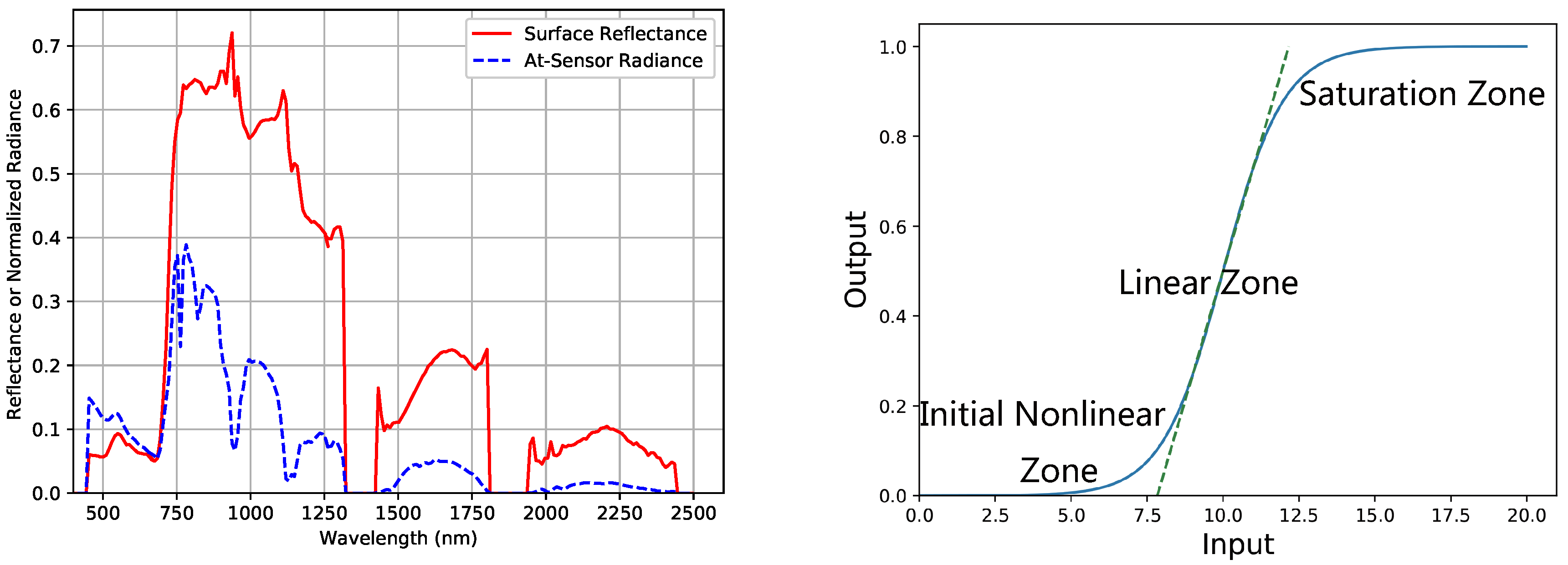
Hyperspectral images provide a complete spectrum for every pixel over the wavelength range from 0.4 to 2.5 μm, and the at-sensor radiance images contain absorption and scattering by atmospheric gases and aerosols. Atmospheric correction is a process in order to remove the atmospheric effects and retrieve the surface reflectance for further applications, such as land cover classification. A sample at-sensor radiance spectrum and the corrected reflectance spectrum from a typical hyperspectral sensor, called Airborne Visible Infrared Imaging Spectrometer (AVIRIS) [1], are shown in Figure 1.
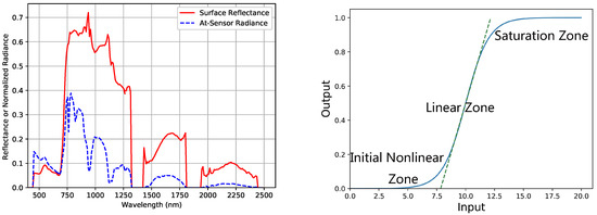
Figure 1.
A sample at-sensor radiance spectrum and the corrected reflectance from AVIRIS dataset (left), and the sensor response function (right). The strong atmospheric absorption regions around 1400 and 1900 nm are excluded.
Several methods [2,3,4] based on radiative transfer model have been developed, including the Fast Line-of-sight Atmospheric Analysis of Spectral Hypercubes (FLAASH) [5] algorithm. These methods calculate the atmospheric effects based on the physical radiative-transfer model and the atmospheric parameters when the hyperspectral image is acquired by sensors. The radiative-transfer model can be expressed by a radiance equation, and the radiance equation of FLAASH is widely used. For each pixel in a hyperspectral image, the standard radiance equation of FLAASH may be written as
Here, and denote the surface reflectance and the at-sensor radiance value at a spectral band centered at wavelength . is the spatially averaged surface reflectance around this pixel, and S is the atmospheric spherical albedo which accounts for enhancement of the ground illumination by atmospheric reflection. A and B are coefficients that only depend on atmospheric and geometric conditions. They respectively account for the Sun-surface-sensor path transmittance and the diffuse transmittance caused by the scattering from surface around this pixel which is regarded as the “adjacency effect”. is the atmospheric scattering transmittance which never encounters the surface but contributes to the at-sensor radiance value. As L is the at-sensor radiance value, A, B, S, , and have to be accurately calculated to retrieve . Typically, for FLAASH, these coefficients are determined from MODTRAN [6] simulations with the sensor parameters given. However, some atmospheric parameters, such as the water vapor and aerosol coefficients, are hard to measure, therefore are estimated from the at-sensor observed image. These estimations are not stable enough across different scenes and atmospheric conditions. In addition, the absolute radiometric calibration of hyperspectral sensor is necessary for all radiative-transfer modeling approaches so that L can be accurately observed. For relative radiometric calibrated hyperspectral sensors without accurate absolute radiometric calibration, the observed value can be modeled as a linear relationship with L:
Here, a and b are the gradient and bias of the linear relationship. Although the response function of sensor is non-linear, the linear zone can be modeled as a linear form (see Figure 1). For spaceborne sensors, the absolute radiometric calibration has to be implemented every three months or more frequently, otherwise the acquired data and retrieved may contain error that cannot be erased by radiative-transfer modeling approaches. Furthermore, for absolute radiometric calibrated sensors, the accuracy of absolute radiometric calibration can still impose restrictions on the overall accuracy.
In Equation (2), A, B, S, and are often considered as a nearly spatial constant for the atmospheric condition varies very slowly inside an image. Typically, the “adjacency effect” has the spatial scale of around 0.5 km, so is usually a slowly varying function across spatial position in a large image. When the image covers a small region (<1 km) or the scene materials in a large image are nearly uniformly distributed, can be considered as a spatial constant. Under this circumstance which frequently applies, Equation (2) reduce to a linear form:
where and .
Based on Equation (3), many empirical approaches have been proposed, such as the empirical line method (ELM) [7]. When combining Equations (2) and (3), the relationship between at-sensor observed value and can still be modeled as a linear form:
where and . Since empirical approaches directly estimate and from the image instead of radiative-transfer model, they do not require absolute radiometric calibration, but they need prior knowledge such as known surface reflectance of some surface materials. Without prior knowledge, QUAC (Quick Atmospheric Correction) [8,9], defined as a semi-empirical method, is based on the key assumption that the average of diverse endmember [10] reflectance spectra is a nearly wavelength-independent constant. However, this assumption is usually not met for images containing around 10 or less spectrally diverse materials and there is still room for improvement.
In recent years, machine learning has achieved state-of-the-art performance on many computer vision problems, such as object identification and image classification. For supervised learning, support vector machine (SVM) [11] and convolutional neural networks (CNNs) [12,13] perform best on most typical datasets, including MNIST [14] (an open database of handwritten digits) and ImageNet [15] (a widely used open dataset for image classification). Most of the works utilizing machine learning on remote sensing focus on application problems, including object recognition [16,17] and image classification [18,19]. Besides, machine learning is also utilized to improve the correction of remote sensing image and parameter retrieval, e.g., SVM has achieved outstanding performance on the bias correction of MODIS aerosol optical depth [20] and the retrieval of biomass and soil moisture [21]. For some retrieval problems, the learning model has to provide prediction for every pixel such as the surface reflectance retrieval, and the traditional CNN becomes impracticable. Hypercolumn [22] based on CNN and fully convolutional networks (FCNs) [23] are designed for solving such dense prediction problems, such as semantic segmentation, object segmentation, and image colorization [24]. Hypercolumn, which is easy to implement on Caffe [25], provides multi-scale spatial features for every pixel. In the experiment of [26], feature generated from ImageNet pre-trained CNN model performs much better than the traditional spatial features on differentiating coffee and non-coffee remote sensing images. This result indicates that the CNN feature generalizes well on remote sensing data and CNN-based hypercolumn can be a good feature descriptor for our problem.
In this paper, we propose a novel method abbreviated as MLAC for hyperspectral atmospheric correction based on machine learning. MLAC can automatically implement correction for a large amount of images from totally different spatial positions and atmospheric conditions which radiative-transfer modeling approaches cannot. As will be explained in Section 2, SVM is utilized to learn the surface reflectance from at-sensor radiance image and hypercolumn is used for feature extraction. After training, the model can automatically predict the surface reflectance of other images without prior knowledge and additional metadata. Just like empirical approaches, MLAC does not require absolute radiometric calibration either. Based on the Equation (4) that the relationship between the spectral reflectance and at-sensor radiance is linear, like empirical approaches and QUAC, MLAC uses a linear fitting for better accuracy after the learning model’s prediction. In Section 3, the experiments are conducted to validate the performance of the proposed method on AVIRIS dataset compared with QUAC and FLAASH, and the difference between MLAC and others are discussed. Finally, Section 4 gives the conclusion and our future works.
2. Approach
2.1. Workflow
According to Equation (4), empirical methods estimate and from the observed images, and then the surface reflectance can be retrieved by . For example, ELM assumes that there are at least two known reflectance spectra within an image so that and can be easily calculated by a linear fitting which will be further explained in Section 2.6. However, the known reflectance spectra come from manual intervention which is not practical for automated correction. Fortunately, machine learning can solve this problem by automatically predicting the for several pixels after training on a labeled dataset (explained in Section 2.3, Section 2.4 and Section 2.5). Although we need corrected surface reflectance data when training the learning models, the trained models can predict reflectance for images from totally different spatial position and atmospheric conditions without additional metadata. To achieve this goal, the preprocessing (explained in Section 2.2) is necessary for input hyperspectral images. The flowchart of MLAC is illustrated in Figure 2.
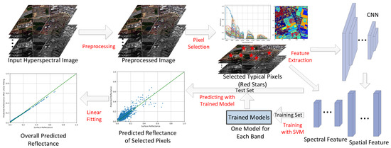
Figure 2.
The flowchart of MLAC.
2.2. Preprocessing
If the learning models predict surface reflectance directly from the at-sensor radiance image, the learning problem can be modeled as
where is the parameters of the learning model f. With the atmospheric conditions changed, the input will nearly vary as a linear form, while f has to keep unchanged which is very difficult. Therefore we preprocess all input images so that the preprocessed at the same spatial position stays nearly unchanged under variant atmospheric conditions (extreme conditions such as thick clouds and fogs are beyond our consideration). In addition, the learning will be easier based on the processed images.
First, the input at-sensor observed images are all cropped into a spatial size of , which is the same as the size of the input data layer in the CNN model for feature extraction. Then, the normalization is implemented band by band for each cropped scene independently,
when . In this equation, denotes normalized value of the cropped scene. In addition, and denote the maximal and the minimal radiance value across the cropped scene. Owing to some anomalous points with reflectance beyond , and in Equation (6) can fluctuate widely and severely degrade the stability of normalization. In our experiment, we use the value of the top and bottom 1% points in each band instead of and in Equation (6), respectively.
2.3. Pixel Selection
For the quantity of materials within an image is usually limited, our method selects several typical pixels of different materials from each image. In our experiment 20 pixels are enough and we use a simple empirical algorithm which is found effective and fast (see Figure 3). In the selecting algorithm, the 224-band AVIRIS spectral radiance data of each pixel is considered to be a 224-dimensional vector v, and V denotes the set of all v within an image. The algorithm flow is illustrated in Algorithm 1, where M denotes the number of pixels to be selected. N is the number of all and P is the set of all selected vectors. D is a matrix which saves the angle between a vector and all and is a N-dimensional vector. The returns the inner product of vectors u and v, and returns the root of a number x. The returns a angle value y so that . The “a ← b” means to assign the value of b to variable a. This algorithm is implemented on all cropped scenes.
| Algorithm 1: Pixel Selection |
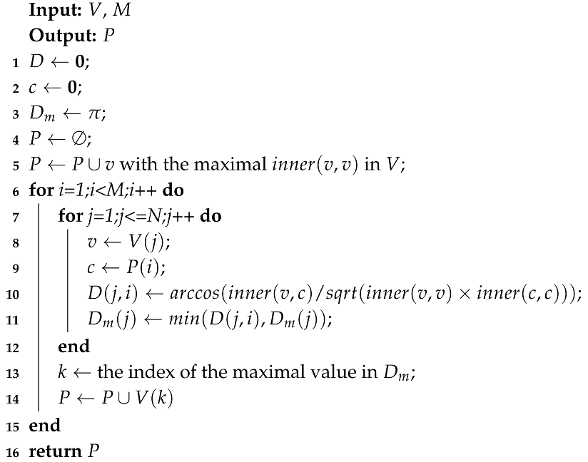 |
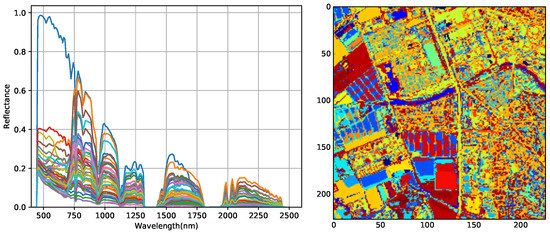
Figure 3.
The selected spectra from an image (left) and the clustering result based on these pixels (right).
2.4. Feature Extraction
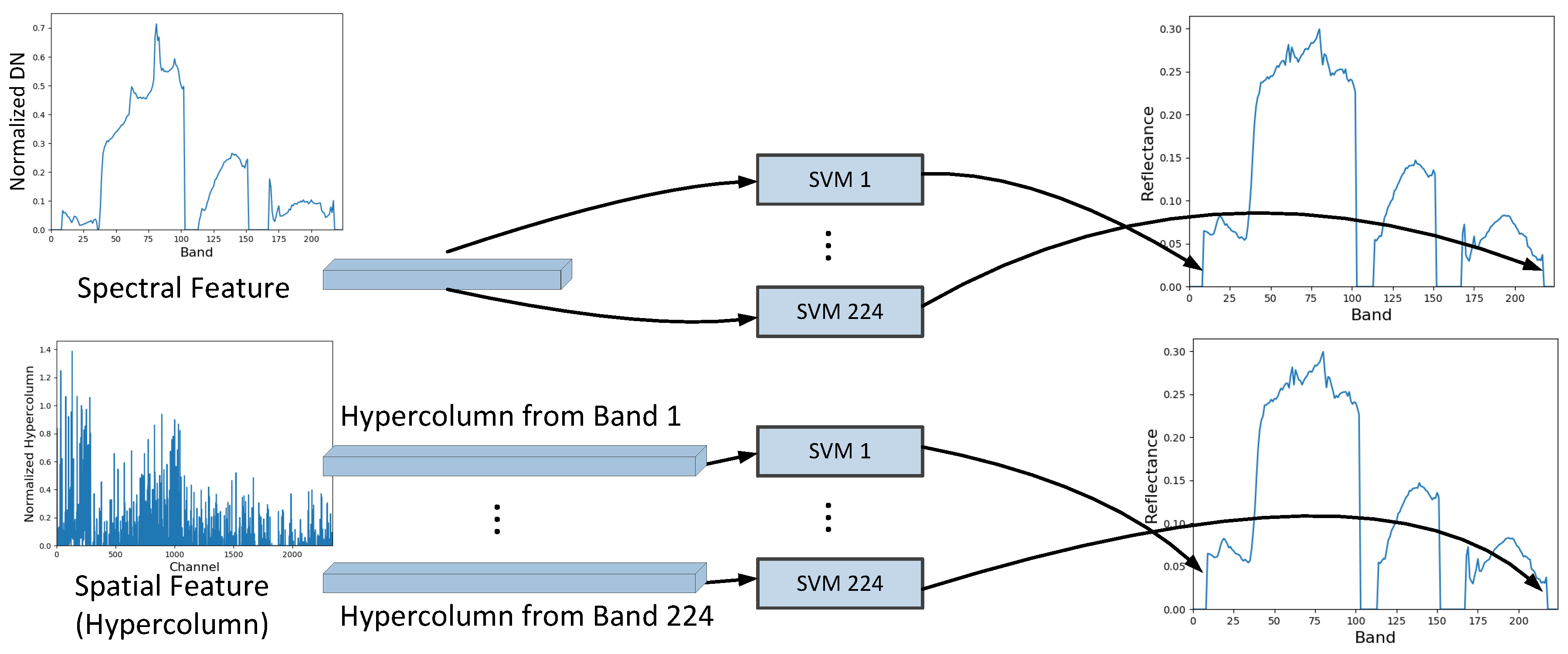
For the selected typical pixel in Section 2.3, their spectral and spatial feature descriptors are extracted for training. Figure 4 shows the whole process of feature extraction. As for AVIRIS data with 224 bands, the preprocessed image still has 224 bands, and for each pixel, the 224 channel values are considered as its spectral feature descriptor without any band selection.
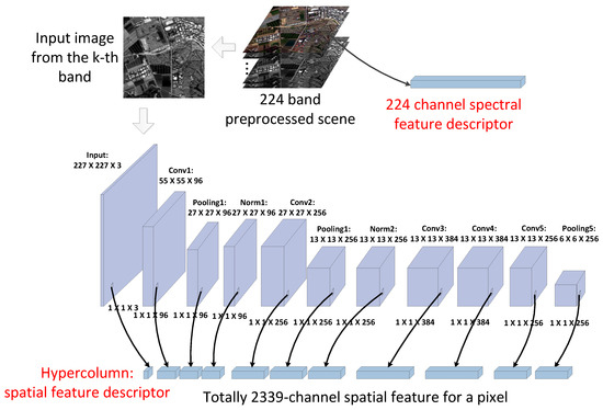
Figure 4.
The spectral and spatial feature descriptor generation.
The CNN model was first proposed for image classification. It contains convolution layers at the bottom for feature extraction and fully connected layers at the top for learning the high-level scene information. Hypercolumn utilizes the results from all layers to build a spatial feature descriptor for all pixels. The CNN model named AlexNet [27], containing five convolutional layers and three fully connected layers, has shown outstanding performance in ILSVRC-2012 (ImageNet Large Scale Visual Recognition Challenge) [15]. In our experiment, one modified version of the AlexNet trained in ILSVRC-2012 competition, called BVLC Reference CaffeNet, is used for generating the hypercolumn [22] as the spatial feature descriptor of each pixel. In addition, the top three fully connected layers are discarded because they represent the high-level semantic properties rather than spatial feature. For each preprocessed scene, the data from a specific band is selected as the input of the CNN model with pre-trained weights, so that the generated hypercolumn represents the spatial feature of this band. Then, the corresponding coordinates of every pixel in different layers are calculated based on the size of each layer, e.g., for a pixel at coordinate in cropped scene, its corresponding coordinate in an layer is calculated by . After the forward calculation of the CNN, the values at these coordinates on all used layers forms the hypercolumn of this pixel as shown in Figure 4. To evaluate the performance of spatial feature alone, the image from the kth band is used as the input for predicting the reflectance of the kth band. The input data layer is considered to be three channels because the input is a grayscale image generated from single-band data. In addition, the five convolution layers with pooling and normalization layers respectively contain , , 384, 384, and channels. So, hypercolumn in our experiment totally contains 2339 channels and the value of each channel is normalized before being used in training. Hypercolumn contains multi-scale spatial feature which has been proved to be effective for colorization and object segmentation [22]. Although the feature maps of higher layers have smaller sizes, they contain important high-level spatial feature which low-level layers cannot provide.
2.5. Training
After feature extraction, SVM models are trained for predicting the surface reflectance from the extracted spectral or spatial feature. SVM was initially designed for classification based on the concept of support vector and decision plane. It has both strong theoretical foundations and abundant empirical successes. In the simplest form of SVM, the hyperplanes are optimized to separate the training data points by a maximal margin and the test data can be classified by these hyperplanes. The data vectors lying close to the hyperplanes are called support vectors. SVR (Support Vector Regression) [28] is an extension of SVM for handling regression problems and usually works with the kernel methods, which map the data into a higher-dimensional space to help handle the non-linear problems. We use the so-called epsilon-SVR [28] with Gaussian kernel to learn the relationship between the reflectance and the spectral and spatial features of all selected pixels. Totally, 224 SVR models are trained for 224 bands (see Figure 5). In addition, when training each model, the input instance data is the spectral or spatial feature descriptor of selected pixels in training set and the input label data is their corresponding surface reflectance of the specific band. The parameter optimization is implemented to find the best parameters for our problem, and the adjustment of parameters can help improve the regularization of SVM to avoid overfitting. After training, the surface reflectance of pixels in test set can be predicted very fast by the trained models.

Figure 5.
The 224 SVM models in training.
2.6. Post-Processing
After predicting the surface reflectance of selected pixels in cropped scenes, the least-square method is used for the linear fitting between the predicted value and at-sensor radiance value of the corresponding band (see Figure 6). The least-square method theoretically minimize the mean squared error between the original points and the fitting line, and the fitting coefficients k and b are calculated as
where and are the input and output arrays. n denotes the length of and , and the fitting equation is written as . It should be pointed out that the linear-fitting coefficients calculated from selected pixels are applicable for other pixels in the same cropped scene according to Equation (4). Furthermore, the linear fitting can be implemented on a group of cropped scenes together, if they are cropped from the same image indicating that they are acquired in a similar atmospheric condition. After the linear fitting, the reflectance of all pixels in the input image is predicted and MLAC is completed.
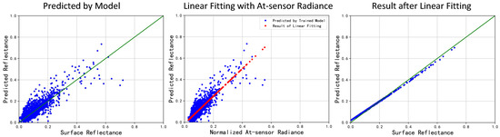
Figure 6.
The reflectance predicted by trained model (left), the linear fitting process (middle) and the predicted result after linear fitting (right).
3. Experiment
3.1. Dataset
We use the AVIRIS surface reflectance product as the ground truth reflectance image for training and the orthorectified product without atmospheric correction is considered to be the input at-sensor radiance image. All these products are provided on the website of NASA (National Aeronautics and Space Administration) JPL (Jet Propulsion Laboratory) for free. Their spatial resolution is around 17 m and most of them are acquired in the western United States. We use totally 530 cropped scenes for training and 80 cropped scenes for validation. When training SVM, the training set contains 10,600 pixels selected from the training cropped scenes by Algorithm 1. This amount of training data is big enough for learning from the high-dimensional spatial feature. After training, MLAC is validated on the test set containing 1600 pixels from the test cropped scenes. All scenes for validation are cropped from the same large image, which is acquired at totally different spatial position and atmospheric conditions from the training cropped scenes. The MODIS [29] land cover type product is used for counting 17 different types of cropped scenes in our dataset. Since the spatial resolution of MODIS data is around 500 m, there are approximately 36 MODIS pixels in each cropped AVIRIS scene. In Table 1, the numbers of MODIS pixels with respect to different land cover types in our dataset are listed and the six MODIS land cover types that are not present are excluded from the table. Since the performance of QUAC and MLAC is sensitive to the number of different materials within a cropped scene rather than the type of a cropped scene, in our experiments, all cropped scenes are further classified into three classes according to the number of different materials.

Table 1.
Numbers of MODIS pixels with different land cover types in our dataset.
3.2. Implementation
In this experiment, the open software named Libsvm [30] is used for implementing SVM and it makes parameter optimization very easy by the cross validation interface (randomly selecting 33% of the training set for cross validation). In addition, the CNN-based hypercolumn is implemented on a deep learning framework called Caffe [25]. Training one model takes approximately 5 min on Intel Core i7-4790 CPU and predicting with the trained model for one cropped scene can be finished in less than half a minute. In addition, the speed of pixel selection can be further improved by parallel computing. QUAC is implemented with the existing function integrated in IDL/ENVI (Interactive Data Language/The Environment for Visualizing Images).
3.3. Result
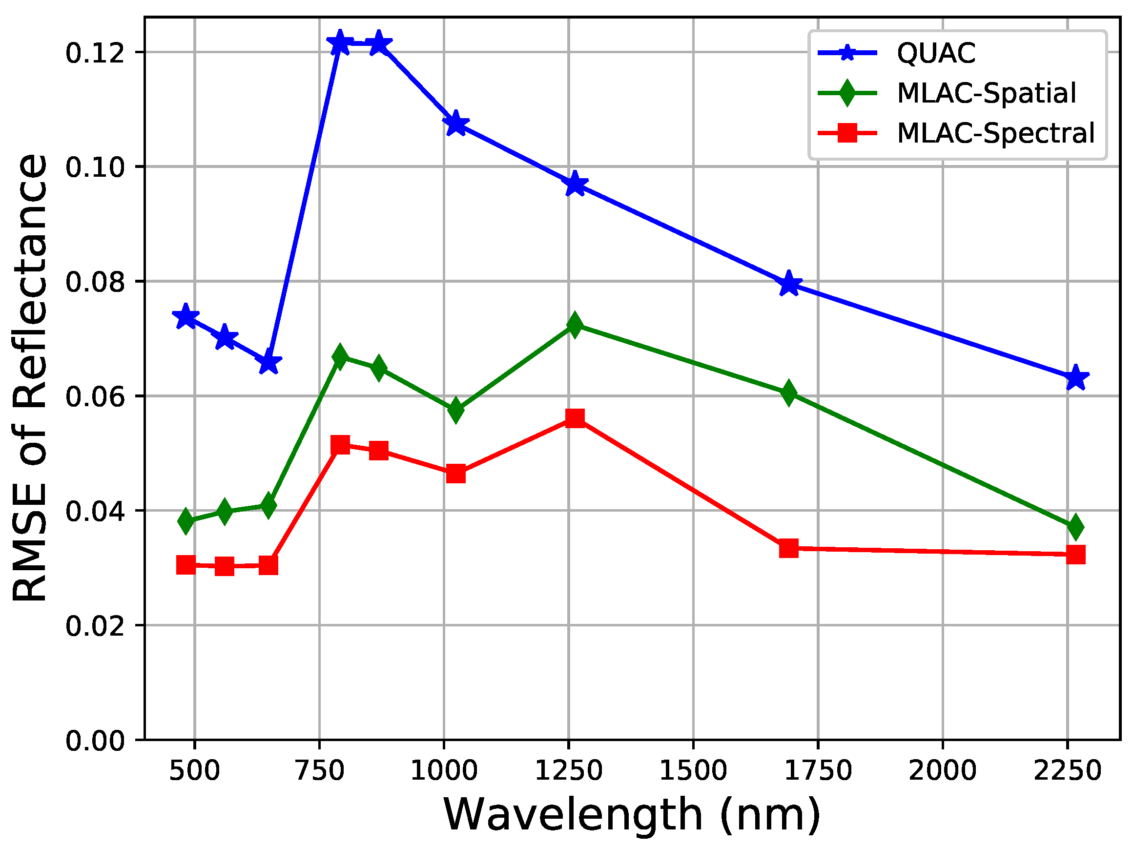
MLAC based on the spectral and spatial feature, respectively, is validated on the 80 test scenes separately and the RMSE (root-mean-square error) of the predicted reflectance on the 1600 pixels in the test set are calculated as the performance matrix. MLAC-Spectral and MLAC-Spatial respectively denote MLAC based on spectral and spatial feature. QUAC is implemented on the test scenes separately and its RMSE on the test set is also calculated for comparison. FLAASH is excluded for the inconvenience of setting parameters for 80 different cropped scenes.
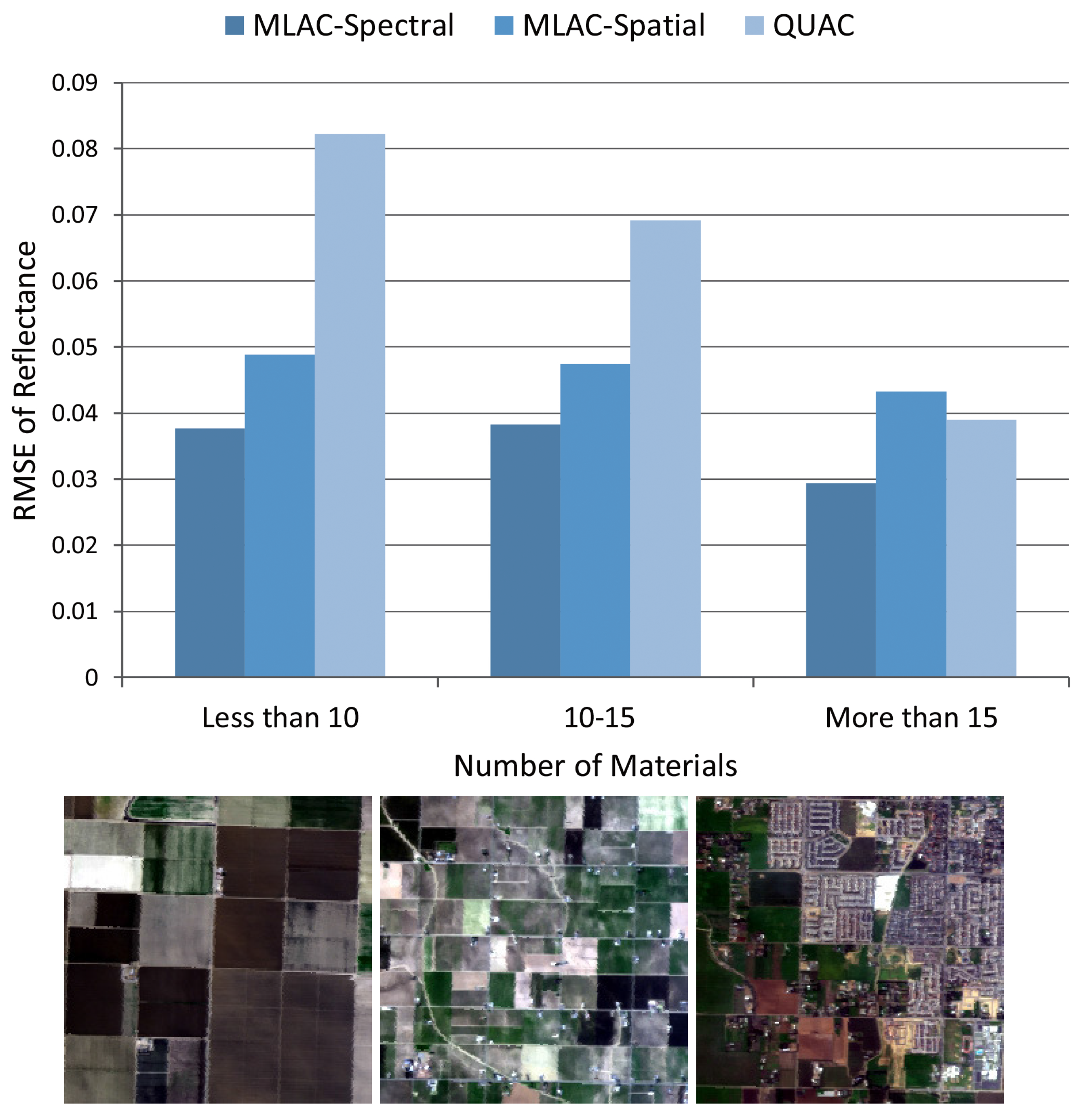
For convenience, the results of nine typical bands (482, 560, 647, 792, 870, 1024, 1263, 1691, and 2267 nm) which can well reflect the overall accuracy are illustrated in Figure 7 indicating that MLAC based on both spectral or spatial feature outperforms QUAC on a variety of scenes. To analyze the results on different scenes, the mean RMSE on all nine bands is calculated for each cropped scene. The result in Figure 8 shows that QUAC performs well on most scenes while being extremely bad on several specific scenes, which usually contain limited materials. To further understand the result, the test scenes are divided into three sets according to the number of materials (less than 10, 10–15, and more than 15) and the mean RMSE of nine bands is calculated on these sets, respectively. In addition, Figure 9 indicates that the performance of QUAC declines as the number of materials decrease in a scene. For scenes containing more than 15 materials, QUAC and MLAC have similar performance, but MLAC based on spectral feature is still the best of them. In a word, MLAC based on spectral and spatial features shows better robustness than QUAC on diverse scenes and the spectral-feature-based one still has better accuracy for scenes containing abundant materials. In addition, the ability to handle diverse scenes with different numbers of materials is very important for automatic retrieval of surface reflectance.
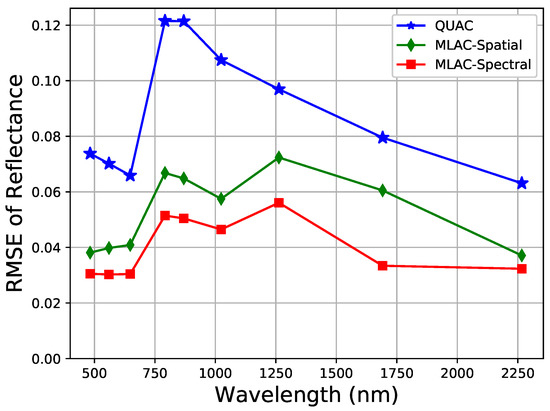
Figure 7.
RMSE of MLAC and QUAC. In the legends of the following figures, “MLAC-Spectral” and “MLAC-Spatial” represent MLAC based on the spectral feature descriptor and hypercolumn.
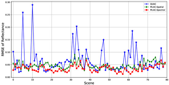
Figure 8.
Mean RMSE of nine typical bands on different scenes.
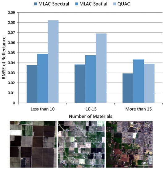
Figure 9.
Mean RMSE of nine typical bands on three classes of scenes and RGB images of typical scenes in each class.
Since the 80 test scenes are cropped from the same image, the post-processing of MLAC can be implemented on all cropped scenes together to improve the accuracy (see Figure 10). QUAC can also get a higher accuracy by implementing on the whole image. In addition, FLAASH is implemented on the whole image and the corresponding RMSE of the test set is calculated. The comparison of their RMSE is shown in Figure 11 indicating that MLAC still works well on handling large image. The spectral-feature-based MLAC outperforms QUAC on most bands and the spatial-feature-based MLAC is still comparable with QUAC. In addition, the result of MLAC-Spectral is comparable with FLAASH.
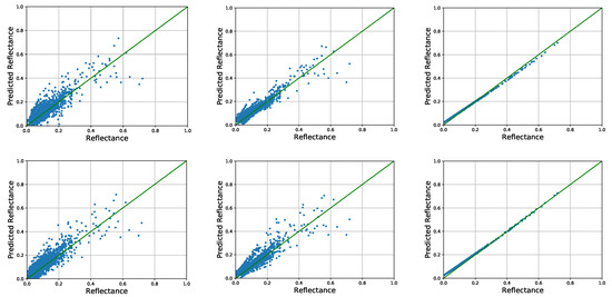
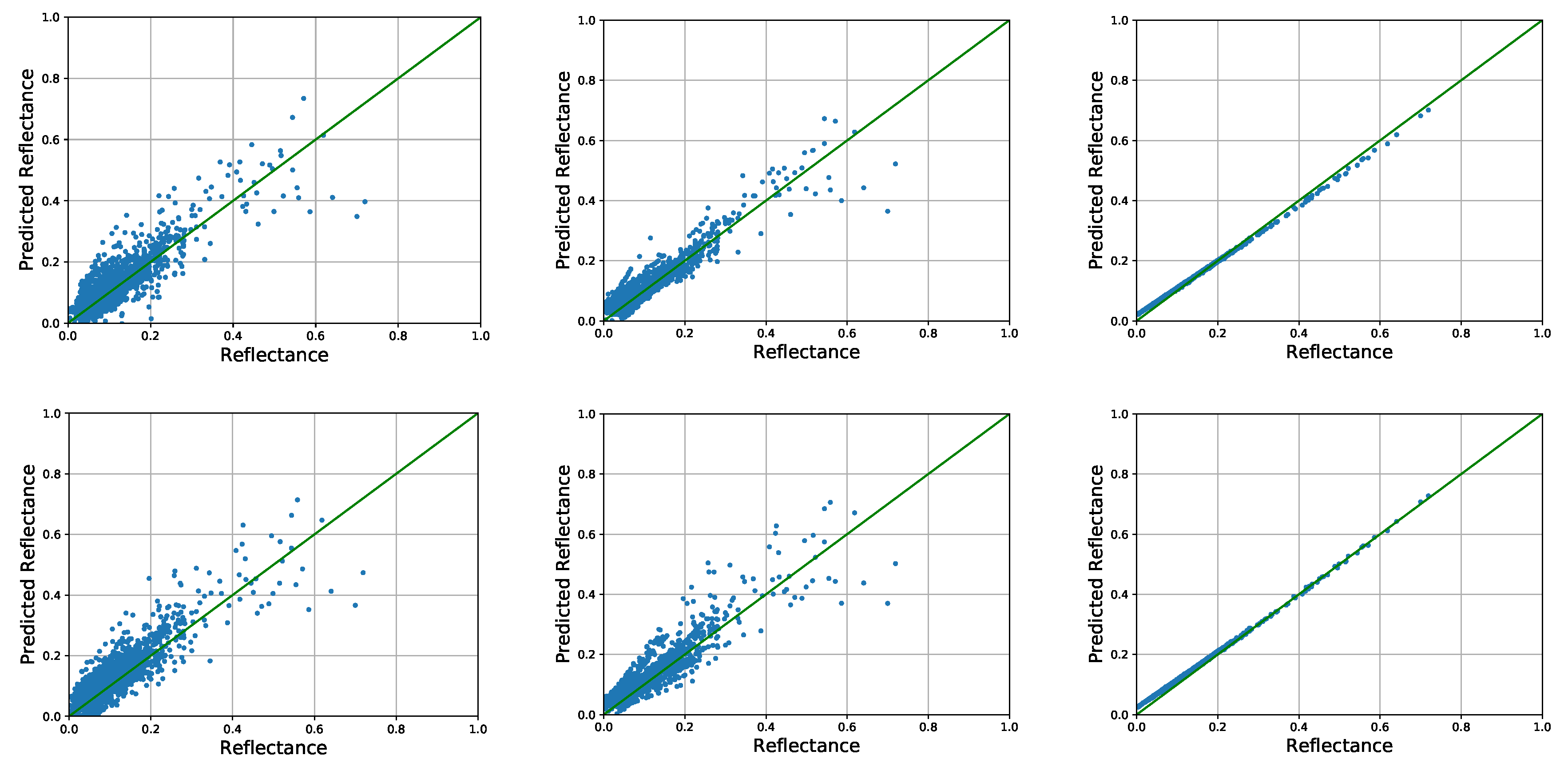
Figure 10.
The original predicted reflectance on 29th band (left), results after linear fitting on different scenes separately (middle), and results after linear fitting on all test scenes together (right). The first row is the result predicted from spectral feature and the second row is from spatial feature.
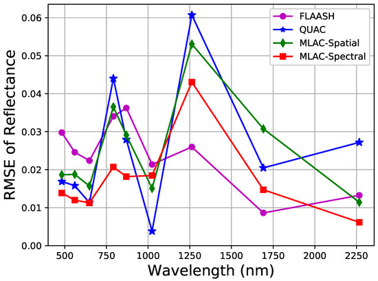
Figure 11.
RMSE of MLAC, FLAASH, and QUAC implemented on the whole test image.
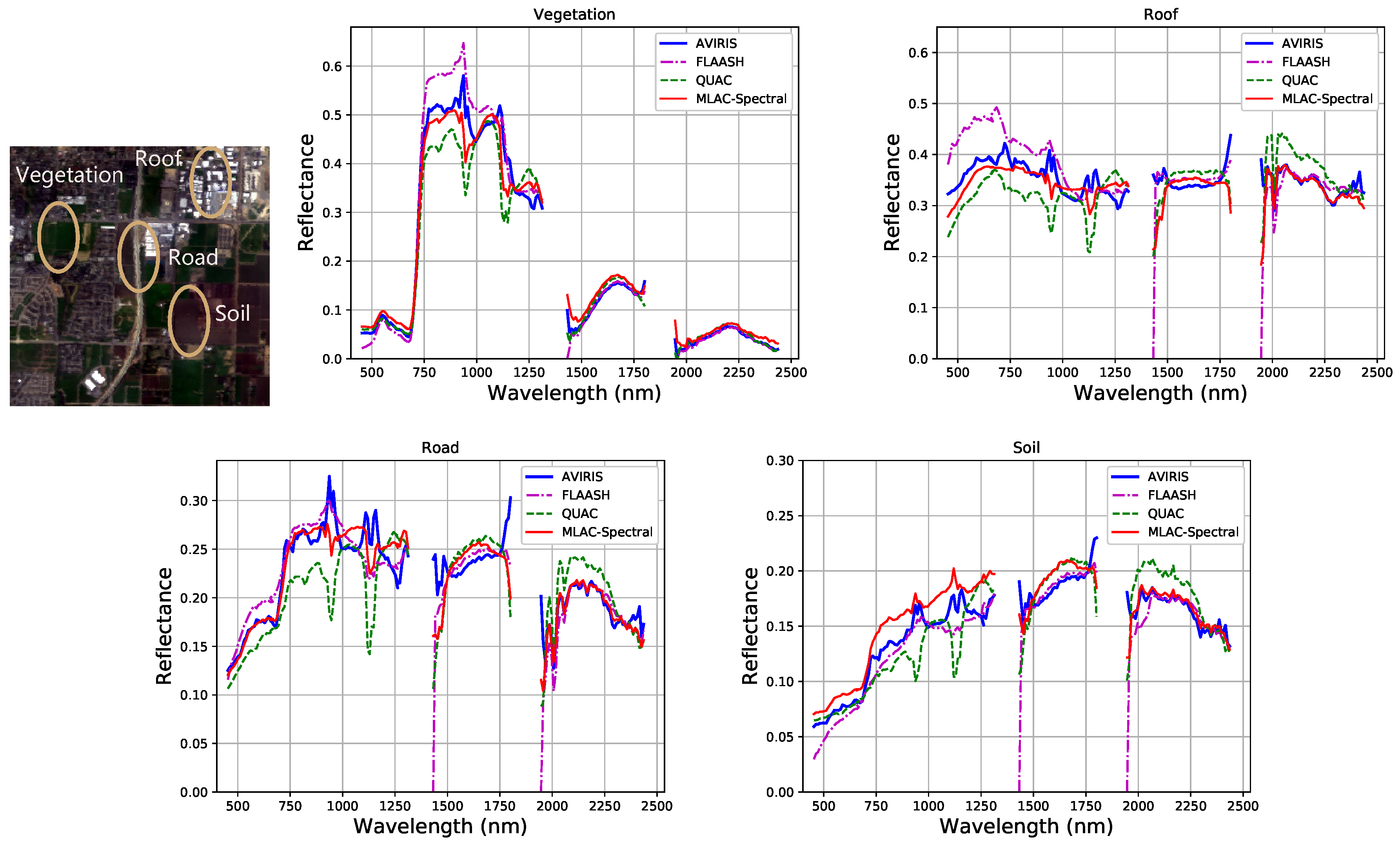
In test scene 52, we select four typical materials (vegetation, roof, road, and soil) and their spectra of all bands generated from MLAC based on spectral feature and QUAC are shown in Figure 12 for detailed comparison. The strong atmospheric absorption regions around 1400 and 1900 nm are excluded because the signal there is too weak. In Figure 12, the result of MLAC based on spectral feature surpasses QUAC on most spectra and the MLAC retrieved spectra have very good agreement with FLAASH and AVIRIS reflectance product. In addition, the result of FLAASH contains large error on some bands such as 780 nm compared with AVIRIS reflectance product. For MLAC, the relative accuracy of dark objects may seem bad, for the prediction offset may be comparable with the reflectance of dark objects. However, the post-processing can be specifically improved to further correct the prediction of dark objects in the future. Although there are also some bad predictions near the strong atmospheric absorption regions, on most bands, the predicted spectra of MLAC are close to the ground truth with absolute accuracy around 0.03 and practicable for further applications.
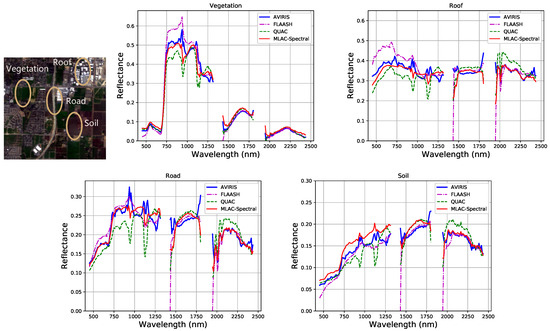
Figure 12.
Spectra generated from MLAC-Spectral, FLAASH, QUAC, and AVIRIS reflectance product on diverse materials.
3.4. Discussion
3.4.1. Our Method vs. Other Methods
The results indicate that MLAC has high accuracy and better robustness across variant scenes compared with QUAC, which is the most widely used method for automated atmospheric correction without setting atmospheric parameters. In addition, the trained model of our method can be theoretically transferred to correct data from brand new sensors, which work on a similar spatial resolution and wavelengths with training data, while QUAC needs a spectral library and cannot work on brand new sensors. Although the training is time-consuming, it only has to be implemented once for application and the time for pixel selection, prediction and linear fitting is comparable with QUAC.
The MLAC-Spectral retrieved spectra have good agreement with FLAASH. Though radiative-transfer model-based methods can achieve high accuracy with the atmospheric parameters precisely measured or estimated, the field measurements may cost a lot and the estimation from images are not stable enough across scenes in variant atmospheric conditions or containing different materials. In addition, some parameters in radiative-transfer model-based methods need manual intervention and depend on prior knowledge, e.g., the “atmospheric model” and “aerosol model” in FLAASH need to be set by human experience. Because of this weakness, radiative-transfer model-based methods are not practical for automated correction on images from totally different spatial positions and atmospheric conditions. In addition, the radiative-transfer model-based methods require accurate absolute radiometric calibration which does not apply in some circumstances. The empirical methods do not require absolute radiometric calibration, but they need prior knowledge thus not practical for automated correction and are not compared in our experiment.
3.4.2. Spectral Feature vs. Spatial Feature
Although the spectral-feature-based method performs better than the spatial-feature-based on accuracy and robustness for correcting hyperspectral images, the latter one still has some advantages for other applications. For example, noting that the spatial-feature-based method only needs data from one band; it can be implemented to images with fewer bands, such as multispectral, optical, and even SAR (Synthetic Aperture Radar) images which the spectral-feature-based method cannot handle. In addition, the spatial-feature-based method will perform better for images with higher spatial resolution. Although theoretically spectral and spatial can work well together, an effective approach to combine spectral and spatial features is yet to be designed for hyperspectral images. The simple connection of two features is confronted with the challenge of the imbalanced dimension and parameter optimization problems.
4. Conclusions
A machine-learning-based method (MLAC) is proposed for atmospheric correction on hyperspectral images and surpasses QUAC in AVIRIS dataset. The retrieved spectra have very good agreement with FLAASH and AVIRIS reflectance product. Several improvements can be implemented in the future for better performance. First, an effective approach to combine spectral and spatial features is yet to be designed for hyperspectral images. In addition, our method does not take into account the error of the AVIRIS reflectance product and cannot eliminate this systemic error. Better ground truth for training can further improve the performance of our methods. Moreover, more improvement can be achieved by increasing the number of diverse scenes in the training set. Although we focus on atmospheric correction in this paper, similar methods can be designed for other retrieval or correction problems.
Acknowledgments
This work was supported by the National Natural Science Foundation of China under Grant No. 61331017.
Author Contributions
Sijie Zhu, Bin Lei, and Yirong Wu conceived and designed the experiments; Sijie Zhu performed the experiments; Bin Lei and Sijie Zhu analyzed the data and result; Sijie Zhu wrote the paper.
Conflicts of Interest
The authors declare no conflict of interest.
References
- Green, R.O.; Eastwood, M.L.; Sarture, C.M.; Chrine, T.G.; Aronsson, M.; Chippendale, B.J.; Faust, J.A.; Pavri, B.E.; Chovit, C.J.; Solis, M. Imaging spectroscopy and the airborne visible/infrared imaging spectrometer (AVIRIS). Remote Sens. Environ. 1998, 65, 227–248. [Google Scholar] [CrossRef]
- Gao, B.C.; Heidebrecht, K.B.; Goetz, A.F. Derivation of scaled surface reflectances from AVIRIS data. Remote Sens. Environ. 1993, 44, 165–178. [Google Scholar] [CrossRef]
- Qu, Z.; Kindel, B.C.; Goetz, A.F. The high accuracy atmospheric correction for hyperspectral data (HATCH) model. IEEE Trans. Geosci. Remote Sens. 2003, 41, 1223–1231. [Google Scholar]
- Kruse, F. Comparison of ATREM, ACORN, and FLAASH atmospheric corrections using low-altitude AVIRIS data of Boulder, CO. In Proceedings of the 13th JPL Airborne Geoscience Workshop, Jet Propulsion Lab, Pasadena, CA, USA, 31 March–2 April 2004. [Google Scholar]
- Cooley, T.; Anderson, G.P.; Felde, G.W.; Hoke, M.L.; Ratkowski, A.J.; Chetwynd, J.H.; Gardner, J.A.; Adler-Golden, S.M.; Matthew, M.W.; Berk, A. FLAASH, a MODTRAN4-based atmospheric correction algorithm, its application and validation. In Proceedings of the IEEE International Geoscience and Remote Sensing Symposium, Toronto, ON, Canada, 24–28 June 2002; Volume 3, pp. 1414–1418. [Google Scholar]
- Adlergolden, S.M.; Matthew, M.W.; Bernstein, L.S.; Levine, R.Y.; Berk, A.; Richtsmeier, S.C.; Acharya, P.K.; Anderson, G.P.; Felde, J.W.; Gardner, J.A. Atmospheric correction for shortwave spectral imagery based on MODTRAN4. Proc SPIE 1999, 3753, 61–69. [Google Scholar]
- Kruse, F.; Kierein-Young, K.; Boardman, J. Mineral mapping at Cuprite, Nevada with a 63-channel imaging spectrometer. Photogramm. Eng. Remote Sens. 1990, 56, 83–92. [Google Scholar]
- Bernstein, L.S.; Adler-Golden, S.M.; Sundberg, R.L.; Levine, R.Y.; Perkins, T.C.; Berk, A.; Ratkowski, A.J.; Felde, G.; Hoke, M.L. A new method for atmospheric correction and aerosol optical property retrieval for VIS-SWIR multi- and hyperspectral imaging sensors: QUAC (QUick atmospheric correction). In Proceedings of the 2005 IEEE International Geoscience and Remote Sensing Symposium, Seoul, Korea, 29 July 2005; Volume 5, pp. 3549–3552. [Google Scholar]
- Bernstein, L.S.; Jin, X.; Gregor, B.; Adler-Golden, S.M. Quick atmospheric correction code: Algorithm description and recent upgrades. Opt. Eng. 2012, 51, 1719. [Google Scholar] [CrossRef]
- Plaza, A.; Martinez, P.; Perez, R.; Plaza, J. A quantitative and comparative analysis of endmember extraction algorithms from hyperspectral data. IEEE Trans. Geosci. Remote Sens. 2004, 42, 650–663. [Google Scholar] [CrossRef]
- Cortes, C.; Vapnik, V. Support-vector networks. Mach. Learn. 1995, 20, 273–297. [Google Scholar] [CrossRef]
- LeCun, Y.; Kavukcuoglu, K.; Farabet, C. Convolutional networks and applications in vision. In Proceedings of the 2010 IEEE International Symposium on Circuits and Systems, Paris, France, 30 May–2 June 2010; pp. 253–256. [Google Scholar]
- Simonyan, K.; Zisserman, A. Very deep convolutional networks for large-scale image recognition. arXiv, 2015; arXiv:1409.1556. [Google Scholar]
- Lecun, Y.; Bottou, L.; Bengio, Y.; Haffner, P. Gradient-based learning applied to document recognition. Proc. IEEE 1998, 86, 2278–2324. [Google Scholar] [CrossRef]
- Russakovsky, O.; Deng, J.; Su, H.; Krause, J.; Satheesh, S.; Ma, S.; Huang, Z.; Karpathy, A.; Khosla, A.; Bernstein, M.; et al. Imagenet large scale visual recognition challenge. Int. J. Comput. Vis. 2015, 115, 211–252. [Google Scholar] [CrossRef]
- Lehtomäki, M.; Jaakkola, A.; Hyyppä, J.; Lampinen, J.; Kaartinen, H.; Kukko, A.; Puttonen, E.; Hyyppä, H. Object Classification and Recognition From Mobile Laser Scanning Point Clouds in a Road Environment. IEEE Trans. Geosci. Remote Sens. 2016, 54, 1226–1239. [Google Scholar] [CrossRef]
- Chen, S.; Wang, H.; Xu, F.; Jin, Y.Q. Target Classification Using the Deep Convolutional Networks for SAR Images. IEEE Trans. Geosci. Remote Sens. 2016, 54, 4806–4817. [Google Scholar] [CrossRef]
- Pasolli, E.; Melgani, F.; Tuia, D.; Pacifici, F.; Emery, W.J. SVM Active Learning Approach for Image Classification Using Spatial Information. IEEE Trans. Geosci. Remote Sens. 2014, 52, 2217–2233. [Google Scholar] [CrossRef]
- Zhang, F.; Du, B.; Zhang, L. Saliency-Guided Unsupervised Feature Learning for Scene Classification. IEEE Trans. Geosci. Remote Sens. 2015, 53, 2175–2184. [Google Scholar] [CrossRef]
- Lary, D.; Remer, L.; MacNeill, D.; Roscoe, B.; Paradise, S. Machine learning and bias correction of MODIS aerosol optical depth. IEEE Geosci. Remote Sens. 2009, 6, 694–698. [Google Scholar] [CrossRef]
- Ali, I.; Greifeneder, F.; Stamenkovic, J.; Neumann, M.; Notarnicola, C. Review of machine learning approaches for biomass and soil moisture retrievals from remote sensing data. Remote Sens. 2015, 7, 16398–16421. [Google Scholar] [CrossRef]
- Hariharan, B.; Arbeláez, P.; Girshick, R.; Malik, J. Hypercolumns for object segmentation and fine-grained localization. In Proceedings of the IEEE Conference on Computer Vision and Pattern Recognition, Boston, MA, USA, 7–12 June 2015; pp. 447–456. [Google Scholar]
- Long, J.; Shelhamer, E.; Darrell, T. Fully convolutional networks for semantic segmentation. In Proceedings of the IEEE Conference on Computer Vision and Pattern Recognition, Boston, MA, USA, 7–12 June 2015; pp. 3431–3440. [Google Scholar]
- Larsson, G.; Maire, M.; Shakhnarovich, G. Learning representations for automatic colorization. In Proceedings of the European Conference on Computer Vision, Amsterdam, The Netherlands, 11–14 October 2016; pp. 577–593. [Google Scholar]
- Jia, Y.; Shelhamer, E.; Donahue, J.; Karayev, S.; Long, J.; Girshick, R.; Guadarrama, S.; Darrell, T. Caffe: Convolutional architecture for fast feature embedding. In Proceedings of the 22nd ACM international conference on Multimedia, Orlando, FL, USA, 3–7 November 2014; pp. 675–678. [Google Scholar]
- Penatti, O.A.; Nogueira, K.; dos Santos, J.A. Do deep features generalize from everyday objects to remote sensing and aerial scenes domains? In Proceedings of the IEEE Conference on Computer Vision and Pattern Recognition Workshops, Boston, MA, USA, 7–12 June 2015; pp. 44–51. [Google Scholar]
- Krizhevsky, A.; Sutskever, I.; Hinton, G.E. ImageNet Classification with Deep Convolutional Neural Networks. In Proceedings of the 25th International Conference on Neural Information Processing Systems, Lake Tahoe, Nevada, 3–6 December 2012; pp. 1097–1105. [Google Scholar]
- Schölkopf, B.; Smola, A.J.; Williamson, R.C.; Bartlett, P.L. New Support Vector Algorithms. Neural Comput. 2000, 12, 1207. [Google Scholar] [CrossRef] [PubMed]
- Salomonson, V.V.; Barnes, W.L.; Maymon, P.W.; Montgomery, H.E.; Ostrow, H. MODIS: Advanced facility instrument for studies of the Earth as a system. IEEE Trans. Geosci. Remote Sens. 1989, 27, 145–153. [Google Scholar] [CrossRef]
- Chang, C.C.; Lin, C.J. LIBSVM: A library for support vector machines. ACM Trans. Intell. Syst. Technol. 2011, 2, 27. [Google Scholar] [CrossRef]


© 2018 by the authors. Licensee MDPI, Basel, Switzerland. This article is an open access article distributed under the terms and conditions of the Creative Commons Attribution (CC BY) license (http://creativecommons.org/licenses/by/4.0/).