Monitoring Sea Level and Topography of Coastal Lagoons Using Satellite Radar Altimetry: The Example of the Arcachon Bay in the Bay of Biscay

 , , ,
, , ,
Abstract

1. Introduction
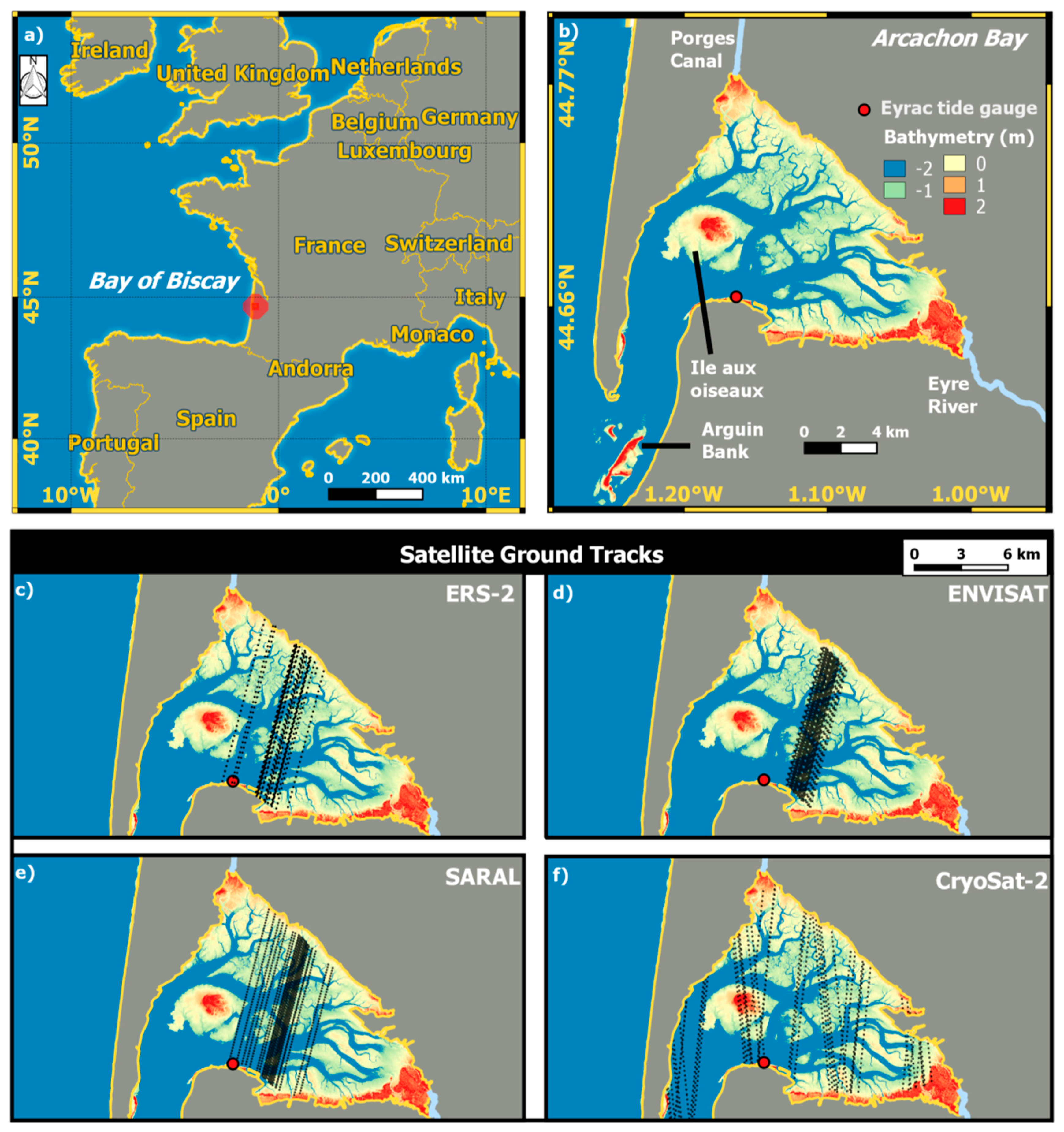
2. Study Area
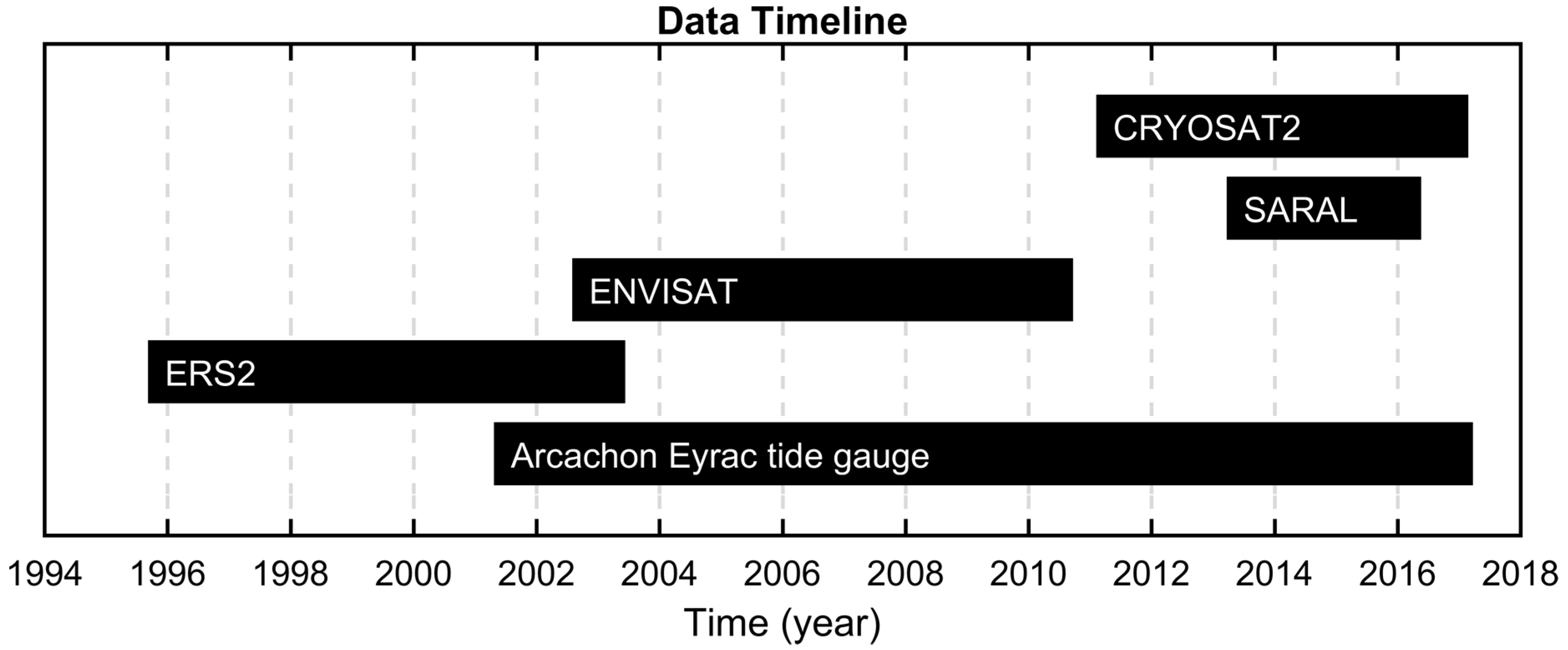
3. Datasets
3.1. Altimetry Data
3.1.1. ERS-2
3.1.2. ENVISAT
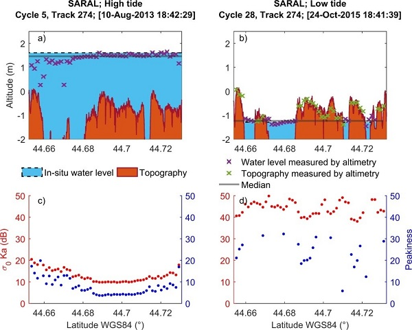
3.1.3. SARAL
3.1.4. CryoSat-2
3.2. Ancillary Data
3.2.1. Arcachon-Eyrac Tide Gauge
3.2.2. Lidar-Derived Topography of the Intertidal Zone
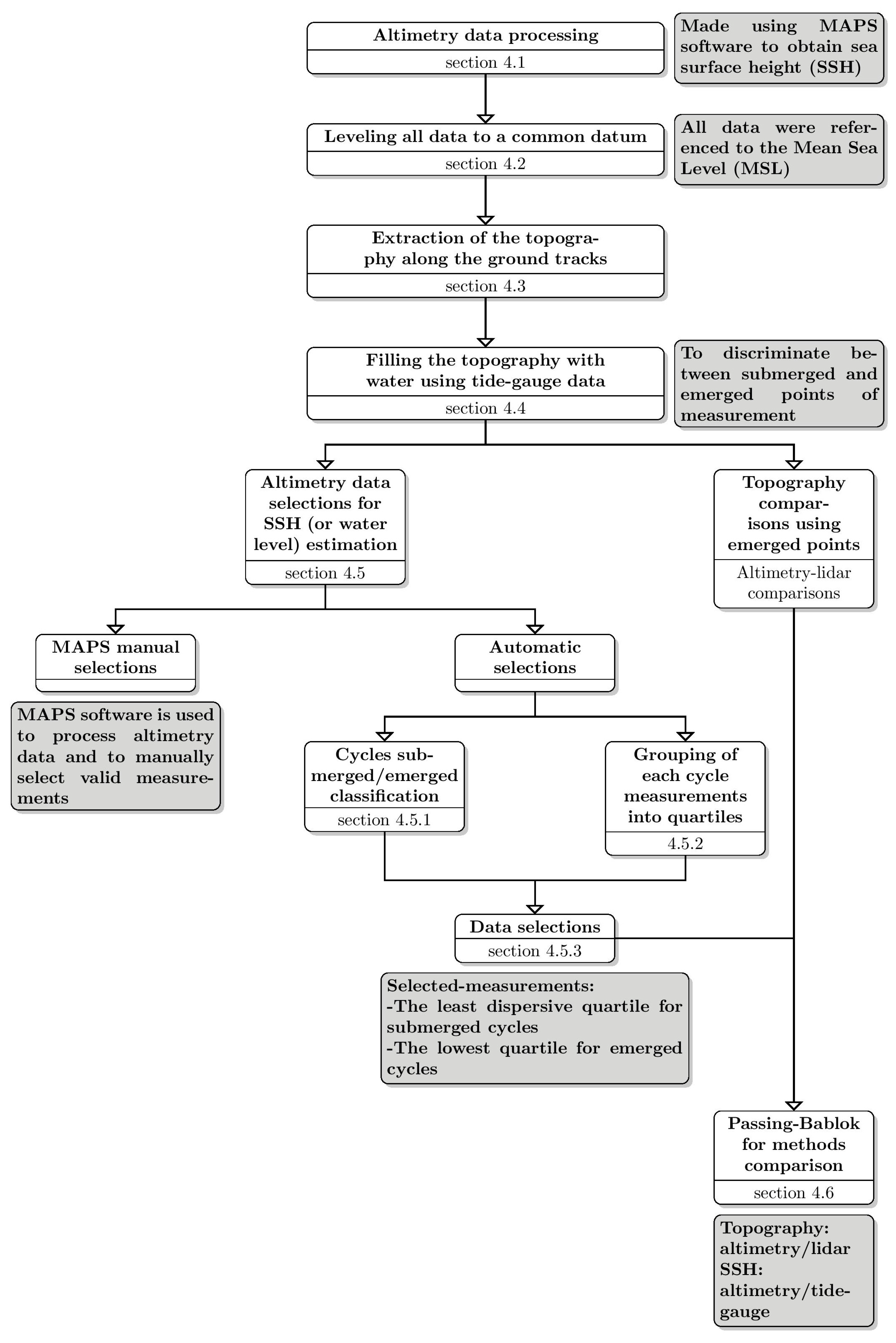
4. Methods
4.1. Altimetry Data Processing
4.2. Leveling to a Common Datum
4.3. Extraction of the Topography of the Intertidal Zone under the Altimeter Tracks
4.4. Manual Classifications of Altimetry Measurements and Cycles
4.5. Automatic Selections of Valid Altimetry Measurements
4.5.1. Classification of Cycles between Submerged and Emerged Cycles
4.5.2. Grouping of Cycle’s Measurements into Four Equal Parts
4.5.3. Data Automatic Selections
4.6. Passing-Bablok Regression for Method Comparisons
4.7. Absolute Calibration of Altimetry Missions over the Intertidal Zone
5. Results
5.1. Auto-Classification Using the k-Means Algorithm
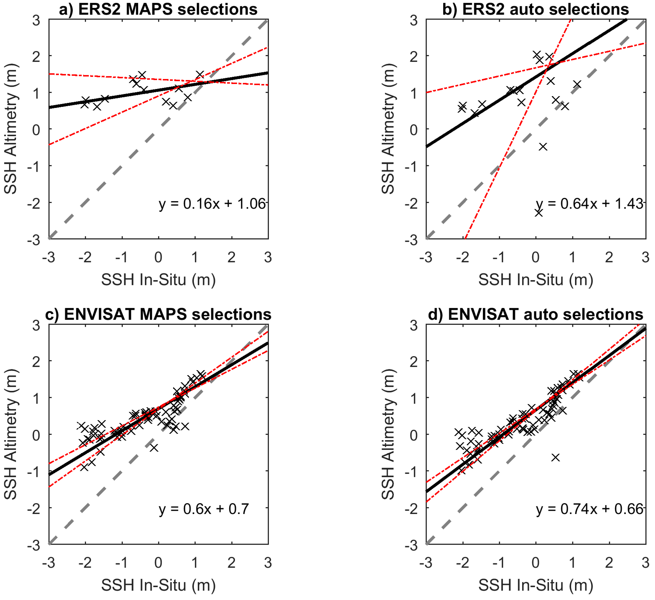
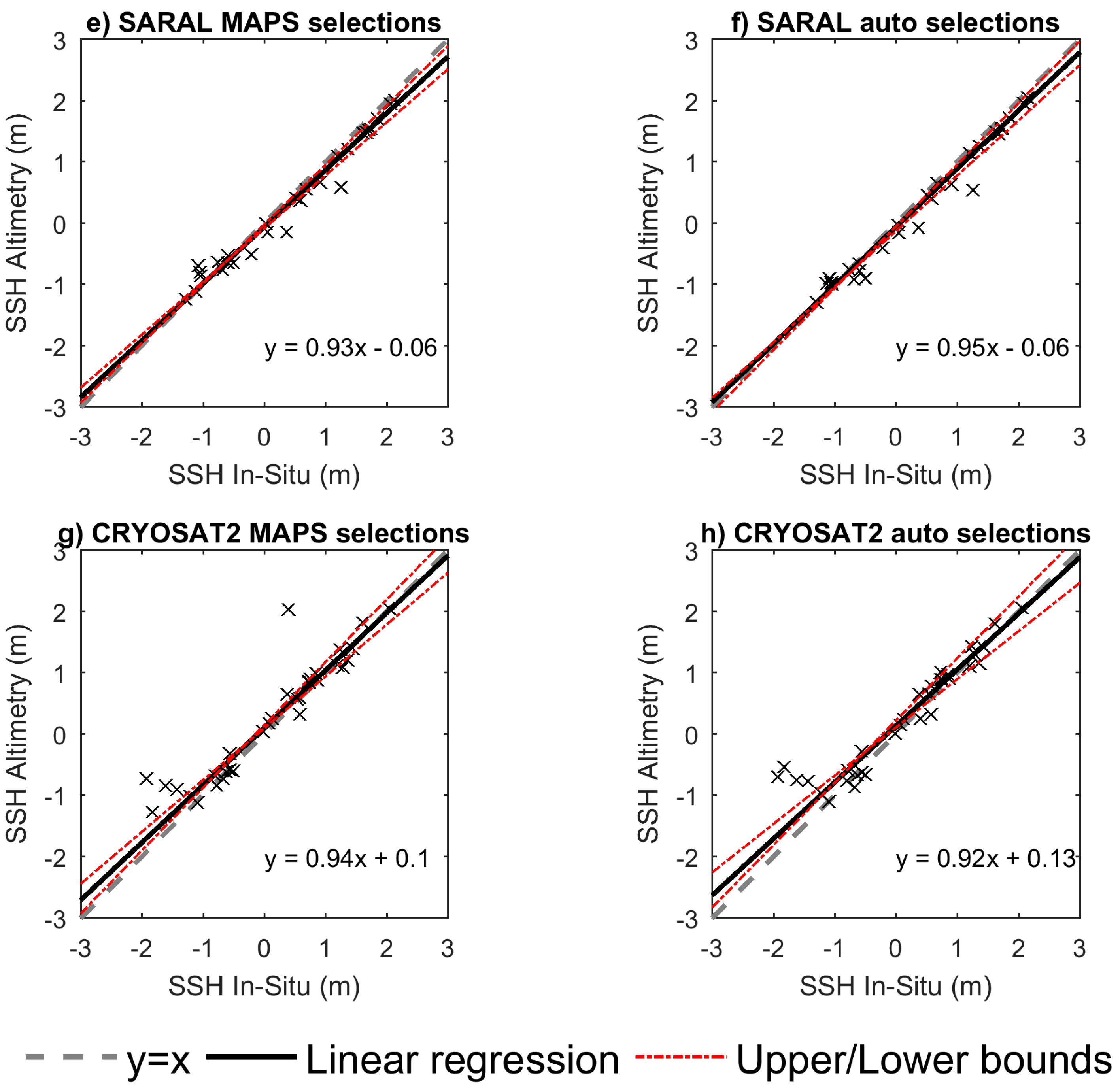
5.2. Water Levels Comparison
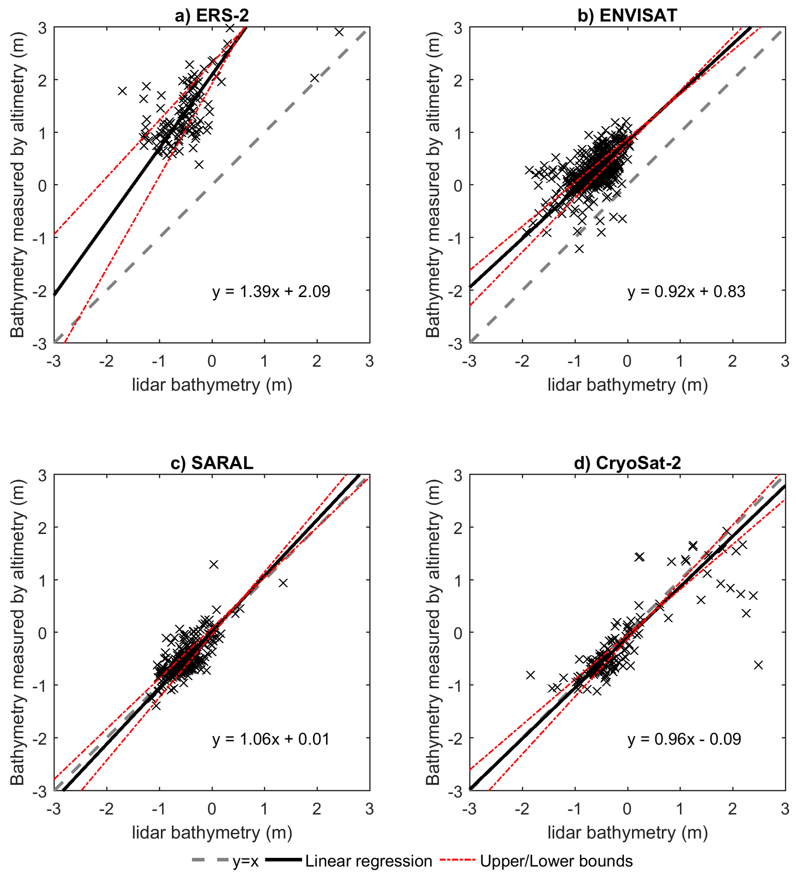
5.3. Topography Comparison
6. Discussion
7. Conclusions
Supplementary Materials
Acknowledgments
Author Contributions
Conflicts of Interest
Appendix A
Appendix B
References
- Agardy, T.; Alder, J. Coastal Systems. In Ecosystems and Human Well-Being: Current State and Trends; Hassan, R., Scholes, R., Ash, N., Eds.; Island Press: Washington, DC, USA, 2005; pp. 513–550. [Google Scholar]
- CIESIN—Center for International Earth Science Information Network. Gridded Population of the World (GPW) Version 3 Beta. Available online: http://sedac.ciesin.columbia.edu (accessed on 20 September 2017).
- Barnes, R.S.K. Coastal Lagoons (Cambridge Studies in Modern Biology 1); Cambridge University Press: Cambridge, UK, 1980. [Google Scholar]
- Kjerfve, B.; Magill, K.E.; Baruch, B.W. Geographic and hydrodynamic characteristics of shallow coastal lagoons. Mar. Geol. 1989, 88, 187–199. [Google Scholar] [CrossRef]
- Chapman, P.M. Management of coastal lagoons under climate change. Estuar. Coast. Shelf Sci. 2012, 110, 32–35. [Google Scholar] [CrossRef]
- Vignudelli, S.; Kostianoy, A.G.; Cipollini, P.; Benveniste, J. (Eds.) Coastal Altimetry; Springer: Berlin/Heidelberg, Germany, 2011. [Google Scholar]
- Cipollini, P.; Calafat, F.M.; Jevrejeva, S.; Melet, A.; Prandi, P. Monitoring Sea Level in the Coastal Zone with Satellite Altimetry and Tide Gauges. Surv. Geophys. 2017, 38, 33–57. [Google Scholar] [CrossRef]
- Deborde, J.; Anschutz, P.; Auby, I.; Glé, C.; Commarieu, M.-V.; Maurer, D.; Lecroart, P.; Abril, G. Role of tidal pumping on nutrient cycling in a temperate lagoon (Arcachon Bay, France). Mar. Chem. 2008, 109, 98–114. [Google Scholar] [CrossRef]
- Plus, M.; Dumas, F.; Stanisiè Re, J.-Y.; Maurer, D. Hydrodynamic characterization of the Arcachon Bay, using model-derived descriptors. Cont. Shelf Res. 2009, 29, 1008–1013. [Google Scholar] [CrossRef]
- Rimmelin, P.; Dumon, J.-C.; Maneux, E.; Gonçalves, A. Study of Annual and Seasonal Dissolved Inorganic Nitrogen Inputs into the Arcachon Lagoon, Atlantic Coast (France). Estuar. Coast. Shelf Sci. 1998, 47, 649–659. [Google Scholar] [CrossRef]
- Blanchet, H.; De Montaudouin, X.; Chardy, P.; Bachelet, G. Structuring factors and recent changes in subtidal macrozoobenthic communities of a coastal lagoon, Arcachon Bay (France). Estuar. Coast. Shelf Sci. 2005, 64, 561–576. [Google Scholar] [CrossRef]
- Envisat, C.Z. RA-2 Advanced Radar Altimeter: Instrument Design and Pre-Launch Performance Assessment Review. Acta Astronaut. 1999, 44, 323–333. [Google Scholar]
- Verron, J.; Sengenes, P.; Lambin, J.; Noubel, J.; Steunou, N.; Guillot, A.; Picot, N.; Coutin-Faye, S.; Sharma, R.; Gairola, R.M.; et al. The SARAL/AltiKa Altimetry Satellite Mission. Mar. Geodesy 2015, 38, 2–21. [Google Scholar] [CrossRef]
- Nielsen, K.; Stenseng, L.; Andersen, O.; Knudsen, P. The Performance and Potentials of the CryoSat-2 SAR and SARIn Modes for Lake Level Estimation. Water 2017, 9, 374. [Google Scholar] [CrossRef]
- Wingham, D.J.; Francis, C.R.; Baker, S.; Bouzinac, C.; Brockley, D.; Cullen, R.; de Chateau-Thierry, P.; Laxon, S.W.; Mallow, U.; Mavrocordatos, C.; et al. CryoSat: A mission to determine the fluctuations in Earth’s land and marine ice fields. Adv. Space Res. 2006, 37, 841–871. [Google Scholar] [CrossRef]
- Frappart, F.; Blumstein, D.; Cazenave, A.; Ramillien, G.; Birol, F.; Morrow, R.; Rémy, F. Satellite Altimetry: Principles and Applications in Earth Sciences. In Wiley Encyclopedia of Electrical and Electronics Engineering; John Wiley & Sons, Inc.: Hoboken, NJ, USA, 2017; pp. 1–25. [Google Scholar]
- Chelton, D.B.; Ries, J.C.; Haines, B.J.; Fu, L.L.; Callahan, P.S. Satellite Altimetry. In Satellite Altimetry and the Earth Sciences: A Handbook of Techniques and Applications; Fu, L.L., Cazenave, A., Eds.; Academic Press: San Diego, CA, USA, 2001; pp. 1–131. [Google Scholar]
- Frappart, F.; Fatras, C.; Mougin, E.; Marieu, V.; Diepkilé, A.T.; Blarel, F.; Borderies, P. Radar altimetry backscattering signatures at Ka, Ku, C, and S bands over West Africa. Phys. Chem. Earth 2015, 83–84, 96–110. [Google Scholar] [CrossRef]
- Frappart, F.; Roussel, N.; Biancale, R.; Martinez Benjamin, J.J.; Mercier, F.; Perosanz, F.; Garate Pasquin, J.; Martin Davila, J.; Perez Gomez, B.; Gracia Gomez, C.; et al. The 2013 Ibiza Calibration Campaign of Jason-2 and SARAL Altimeters. Mar. Geodesy 2015, 38, 219–232. [Google Scholar] [CrossRef]
- Biancamaria, S.; Frappart, F.; Leleu, A.-S.; Marieu, V.; Blumstein, D.; Desjonquères, J.-D.; Boy, F.; Sottolichio, A.; Valle-Levinson, A. Satellite radar altimetry water elevations performance over a 200 m wide river: Evaluation over the Garonne River. Adv. Space Res. 2017, 59, 128–146. [Google Scholar] [CrossRef]
- Frappart, F.; Papa, F.; Marieu, V.; Malbeteau, Y.; Jordy, F.; Calmant, S.; Durand, F.; Bala, S. Preliminary Assessment of SARAL/AltiKa Observations over the Ganges-Brahmaputra and Irrawaddy Rivers. Mar. Geodesy 2015, 38, 568–580. [Google Scholar] [CrossRef]
- Gaspar, P.; Ogor, F.; Le Traon, P.-Y.; Zanife, O.-Z. Estimating the sea state bias of the TOPEX and POSEIDON altimeters from crossover differences. J. Geophys. Res. 1994, 99, 24981–24994. [Google Scholar] [CrossRef]
- Parisot, J.-P.; Diet-Davancens, J.; Sottolichio, A.; Crosland, E.; Drillon, C.; Verney, R. Modélisation des agitations dans le bassin d’Arcachon. Xèmes Journées Sophia Antip. 2008, 435–444. [Google Scholar] [CrossRef]
- Cartwright, D.E.; Edden, A.C. Corrected Tables of Tidal Harmonics. Geophys. J. R. Astron. Soc. 1973, 33, 253–264. [Google Scholar] [CrossRef]
- Wahr, J.M. Deformation induced by polar motion. J. Geophys. Res. Solid Earth 1985, 90, 9363–9368. [Google Scholar] [CrossRef]
- Wingham, D.J.; Rapley, C.G.; Griffiths, H. New Techniques in Satellite Altimeter Tracking Systems. In Proceedings of the IGARSS 86 Symposium, Zurich, Switzerland, 8–11 September 1986; pp. 1339–1344. [Google Scholar]
- Bamber, J.L. Ice sheet altimeter processing sheme. Int. J. Remote Sens. 1994, 15, 925–938. [Google Scholar] [CrossRef]
- Frappart, F.; Minh, K.D.; L’hermitte, J.; Cazenave, A.; Ramillien, G.; Le Toan, T.; Mognard-Campbell, N. Water volume change in the lower Mekong from satellite altimetry and imagery data. Geophys. J. Int. 2006, 167, 570–584. [Google Scholar] [CrossRef]
- Frappart, F.; Calmant, S.; Cauhopé, M.; Seyler, F.; Cazenave, A. Preliminary results of ENVISAT RA-2-derived water levels validation over the Amazon basin. Remote Sens. Environ. 2006, 100, 252–264. [Google Scholar] [CrossRef]
- Laxon, S. Sea ice altimeter processing scheme at the EODC. Int. J. Remote Sens. 1994, 15, 915–924. [Google Scholar] [CrossRef]
- Jekeli, C. Geometric Reference System in Geodesy; Division of Geodesy and Geospatial Science School of Earth Sciences, Ohio State University: Columbus, OH, USA, 2006. [Google Scholar]
- SHOM. Références Altimétriques Maritimes (RAM). Available online: http://diffusion.shom.fr/ (accessed on 10 February 2018).
- Hartigan, J.A.; Wong, M.A. A K-Means Clustering Algorithm. J. R. Stat. Soc. 1979, 28, 100–108. [Google Scholar]
- Craw, S. Manhattan Distance. In Encyclopedia of Machine Learning; Sammut, C., Webb, G.I., Eds.; Springer Science & Business Media: Boston, MA, USA, 2011. [Google Scholar]
- Passing, H.; Bablok, W. A new biometrical procedure for testing the equality of measurements from two different analytical methods. J. Clin. Chem. Clin. Biochem. 1983, 21, 709–720. [Google Scholar] [PubMed]
- Cancet, M.; Bijac, S.; Chimot, J.; Bonnefond, P.; Jeansou, E.; Laurain, O.; Lyard, F.; Bronner, E.; Féménias, P. Regional in situ validation of satellite altimeters: Calibration and cross-calibration results at the Corsican sites. Adv. Space Res. 2013, 51, 1400–1417. [Google Scholar] [CrossRef]
- Ménard, Y.; Jeansou, E.; Vincent, P. Calibration of the TOPEX/POSEIDON altimeters at Lampedusa: Additional results at Harvest. J. Geophys. Res. 1994, 99, 24487. [Google Scholar] [CrossRef]
- Vu, P.; Frappart, F.; Darrozes, J.; Marieu, V.; Blarel, F.; Ramillien, G.; Bonnefond, P.; Birol, F.; Blarel, F. Multi-Satellite Altimeter Validation along the French Atlantic Coast in the Southern Bay of Biscay from ERS-2 to SARAL. Remote Sens. 2018, 10, 93. [Google Scholar] [CrossRef]
- Bonnefond, P.; Verron, J.; Aublanc, J.; Babu, K.; Bergé-Nguyen, M.; Cancet, M.; Chaudhary, A.; Crétaux, J.-F.; Frappart, F.; Haines, B.; et al. The Benefits of the Ka-Band as Evidenced from the SARAL/AltiKa Altimetric Mission: Quality Assessment and Unique Characteristics of AltiKa Data. Remote Sens. 2018, 10, 83. [Google Scholar] [CrossRef]
- Liu, Y.; Kerkering, H.; Weisberg, R.H. Coastal Ocean Observing Systems; Elsevier (Academic Press): London, UK, 2015. [Google Scholar]
- Ulaby, F.; Moore, R.; Fung, A. Microwave Remote Sensing: Active and Passive. Volume 2, Radar Remote Sensing and Surface Scattering and Emission Theory; Addison-Wesley: Boston, MA, USA, 1982. [Google Scholar]
- Hallikainen, M.; Ulaby, F.; Dobson, M.; El-rayes, M.; Wu, L. Microwave Dielectric Behavior of Wet Soil-Part 1: Empirical Models and Experimental Observations. IEEE Trans. Geosci. Remote Sens. 1985, GE-23, 25–34. [Google Scholar] [CrossRef]


| Mission | ERS-2 | ENVISAT | SARAL | CryoSat-2 |
|---|---|---|---|---|
| Agency | ESA | ESA | CNES/ISRO | ESA |
| Launch on | 21/04/1995 | 01/03/2002 | 25/02/2013 | 08/04/2010 |
| End date | 06/07/2011 | 08/06/2012 | Present | Present |
| Altimeter name | RA | RA-2 | AltiKa | SIRAL |
| Radar frequency | Ku-band | Ku and S-bands | Ka-band | Ku-band |
| Altitude | 785 km | 790 km | 790 km | 717 km |
| Orbit inclination | 98.52° | 98.54° | 98.54° | 92° |
| Repetitivity | 35 days | 35 days | 35 days | 369 days |
| Ground-track spacing at the equator | 85 km | 85 km | 85 km | 7.5 km |
| Along track sampling | 20 Hz (350 m) | 18 Hz (~400 m) | 40 Hz (175 m) | 20 Hz (350 m) |
| Mission | MAPS | Auto | ||||||
|---|---|---|---|---|---|---|---|---|
| ERS-2 | ENVISAT | SARAL | CryoSat-2 | ERS-2 | ENVISAT | SARAL | CryoSat-2 | |
| Linearity 3 | 1 | 0 | 1 | 1 | 1 | 1 | 1 | 1 |
| Slope | 0.16 | 0.60 | 0.93 | 0.94 | 0.64 | 0.74 | 0.95 | 0.92 |
| Slope LB 1 | −0.05 | 0.51 | 0.87 | 0.85 | 0.23 | 0.67 | 0.91 | 0.79 |
| Slope UB 2 | 0.44 | 0.71 | 0.97 | 1.02 | 2.07 | 0.83 | 1.01 | 1.01 |
| Intercept | 1.06 | 0.70 | −0.06 | 0.10 | 1.43 | 0.66 | −0.06 | 0.13 |
| Intercept LB | 1.36 | 0.74 | −0.09 | 0.10 | 1.68 | 0.69 | −0.13 | 0.11 |
| Intercept UB | 0.91 | 0.69 | −0.02 | 0.15 | 1.02 | 0.65 | −0.05 | 0.22 |
| R | 0.39 | 0.82 | 0.99 | 0.93 | 0.11 | 0.86 | 0.99 | 0.95 |
| RMSE (m) | 1.75 | 1.04 | 0.23 | 0.42 | 1.70 | 0.92 | 0.22 | 0.39 |
| Mean Bias (m) | 1.47 | 0.88 | 0.18 | 0.23 | 1.50 | 0.79 | 0.17 | 0.24 |
| Mission | ERS-2 | ENVISAT | SARAL | CryoSat-2 |
|---|---|---|---|---|
| Linearity Test 3 | 1 | 0 | 1 | 1 |
| Slope | 1.39 | 0.92 | 1.06 | 0.96 |
| Slope LB 1 | 1.08 | 0.84 | 0.96 | 0.86 |
| Slope UB 2 | 1.75 | 1.02 | 1.19 | 1.09 |
| Intercept | 2.09 | 0.83 | 0.01 | −0.09 |
| Intercept LB | 2.31 | 0.89 | 0.08 | −0.04 |
| Intercept UB | 1.92 | 0.77 | −0.04 | −0.13 |
| R | 0.17 | 0.54 | 0.71 | 0.79 |
| RMSE (m) | 2.01 | 0.95 | 0.23 | 0.44 |
| Mean Bias (m) | 1.93 | 0.90 | 0.17 | 0.25 |
© 2018 by the authors. Licensee MDPI, Basel, Switzerland. This article is an open access article distributed under the terms and conditions of the Creative Commons Attribution (CC BY) license (http://creativecommons.org/licenses/by/4.0/).
Share and Cite
Salameh, E.; Frappart, F.; Marieu, V.; Spodar, A.; Parisot, J.-P.; Hanquiez, V.; Turki, I.; Laignel, B. Monitoring Sea Level and Topography of Coastal Lagoons Using Satellite Radar Altimetry: The Example of the Arcachon Bay in the Bay of Biscay. Remote Sens. 2018, 10, 297. https://doi.org/10.3390/rs10020297
Salameh E, Frappart F, Marieu V, Spodar A, Parisot J-P, Hanquiez V, Turki I, Laignel B. Monitoring Sea Level and Topography of Coastal Lagoons Using Satellite Radar Altimetry: The Example of the Arcachon Bay in the Bay of Biscay. Remote Sensing. 2018; 10(2):297. https://doi.org/10.3390/rs10020297
Chicago/Turabian StyleSalameh, Edward, Frédéric Frappart, Vincent Marieu, Alexandra Spodar, Jean-Paul Parisot, Vincent Hanquiez, Imen Turki, and Benoit Laignel. 2018. "Monitoring Sea Level and Topography of Coastal Lagoons Using Satellite Radar Altimetry: The Example of the Arcachon Bay in the Bay of Biscay" Remote Sensing 10, no. 2: 297. https://doi.org/10.3390/rs10020297
APA StyleSalameh, E., Frappart, F., Marieu, V., Spodar, A., Parisot, J.-P., Hanquiez, V., Turki, I., & Laignel, B. (2018). Monitoring Sea Level and Topography of Coastal Lagoons Using Satellite Radar Altimetry: The Example of the Arcachon Bay in the Bay of Biscay. Remote Sensing, 10(2), 297. https://doi.org/10.3390/rs10020297