An Information Entropy-Based Sensitivity Analysis of Radar Sensing of Rough Surface


Abstract
1. Introduction
2. Materials and Methods
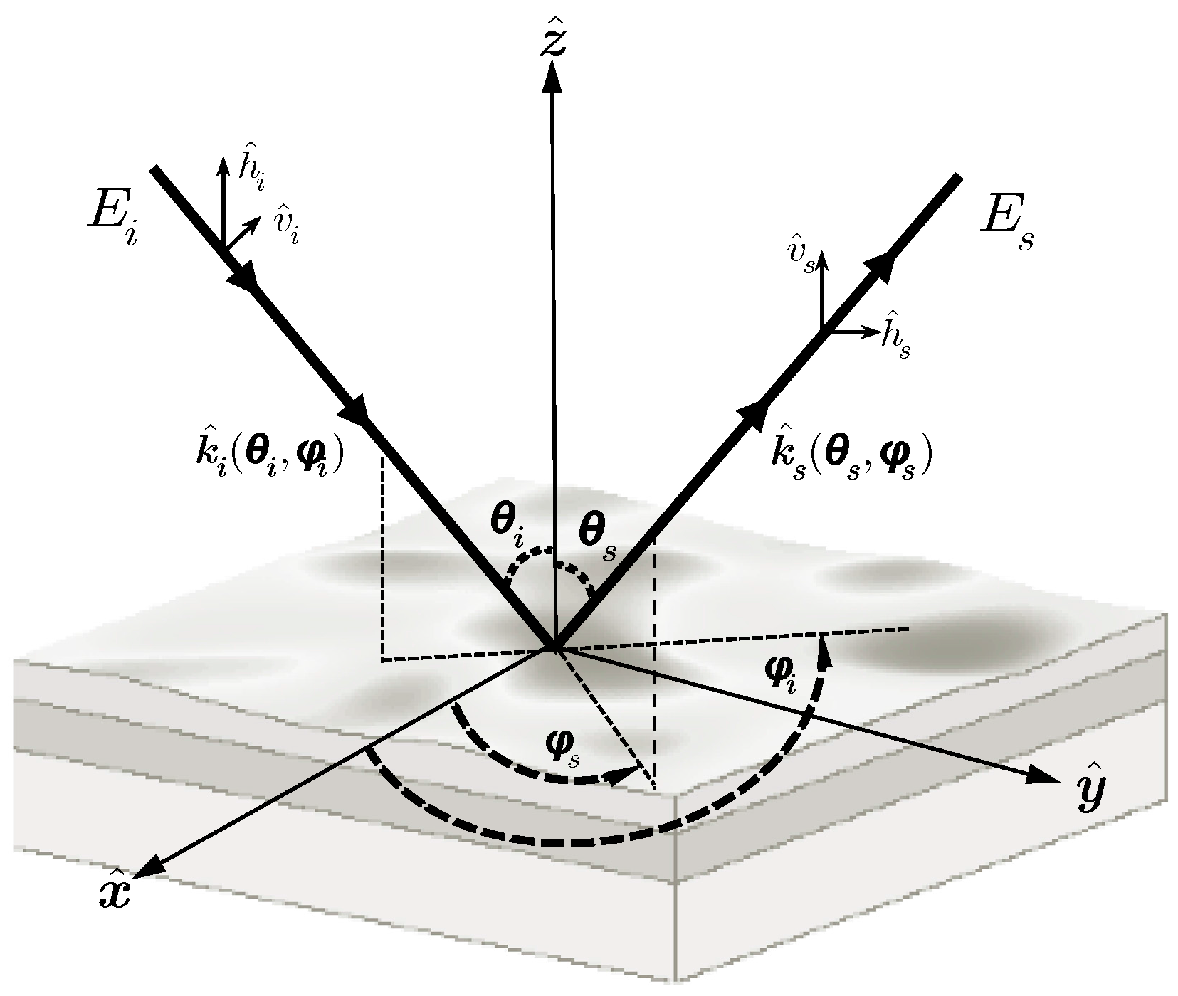
2.1. Surface Scattering Model
2.2. Information Theoretic Criteria
3. Results
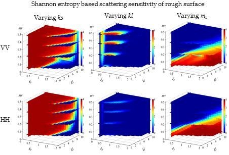
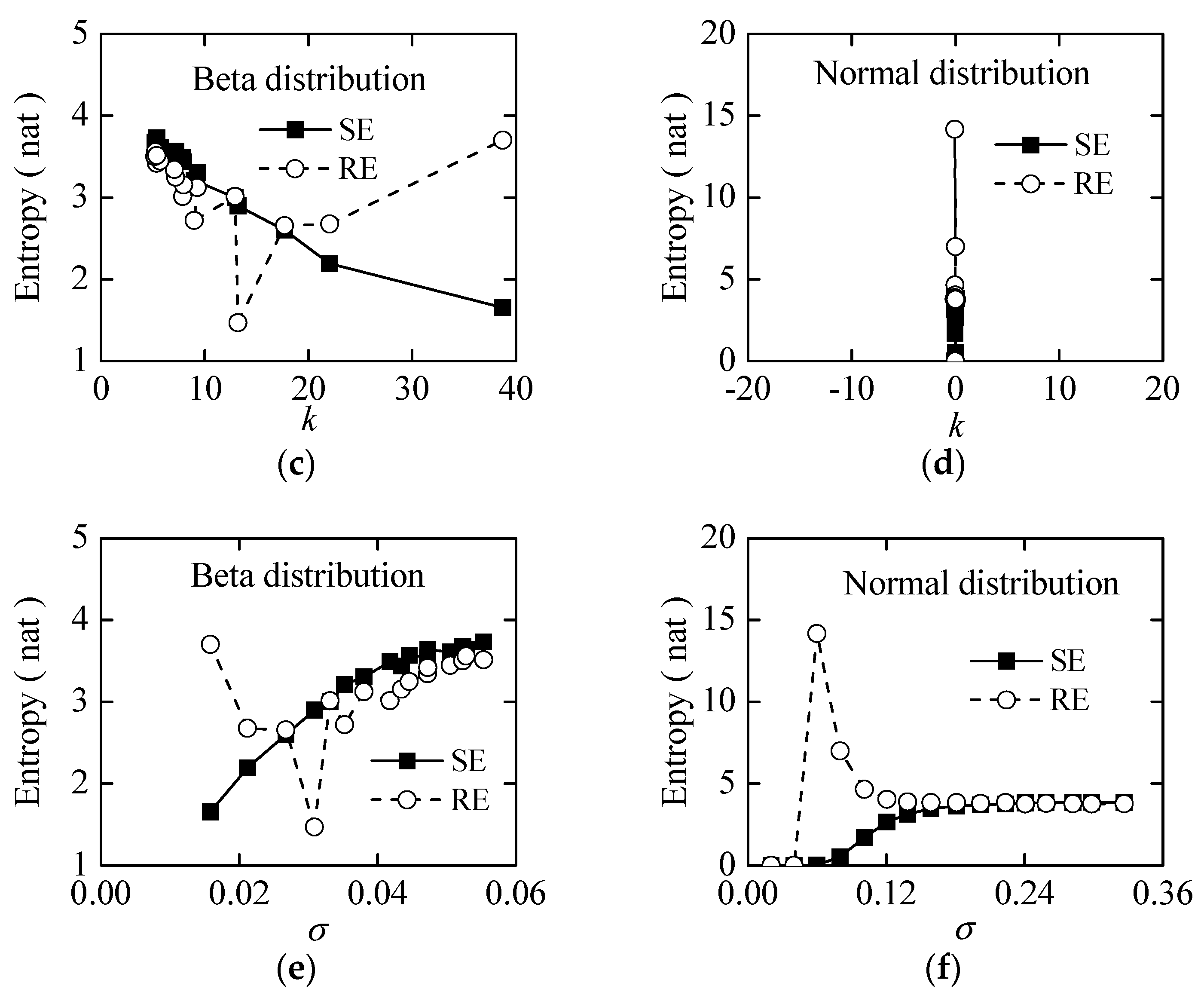
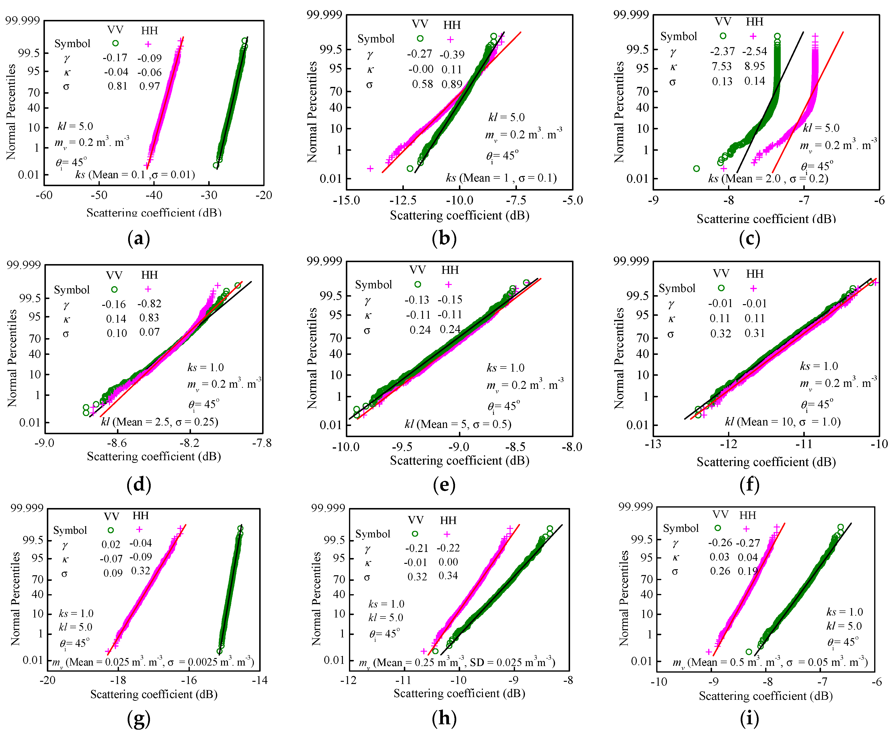
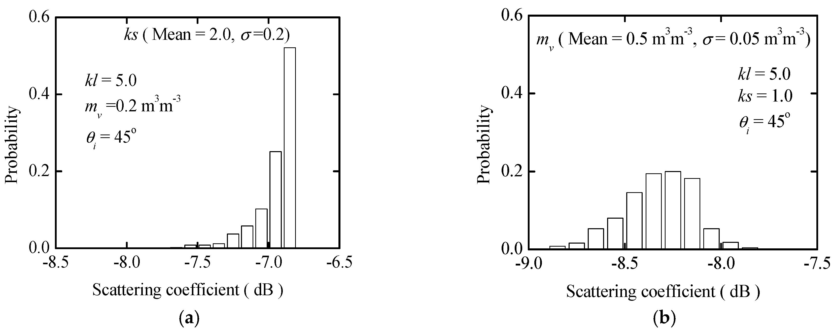
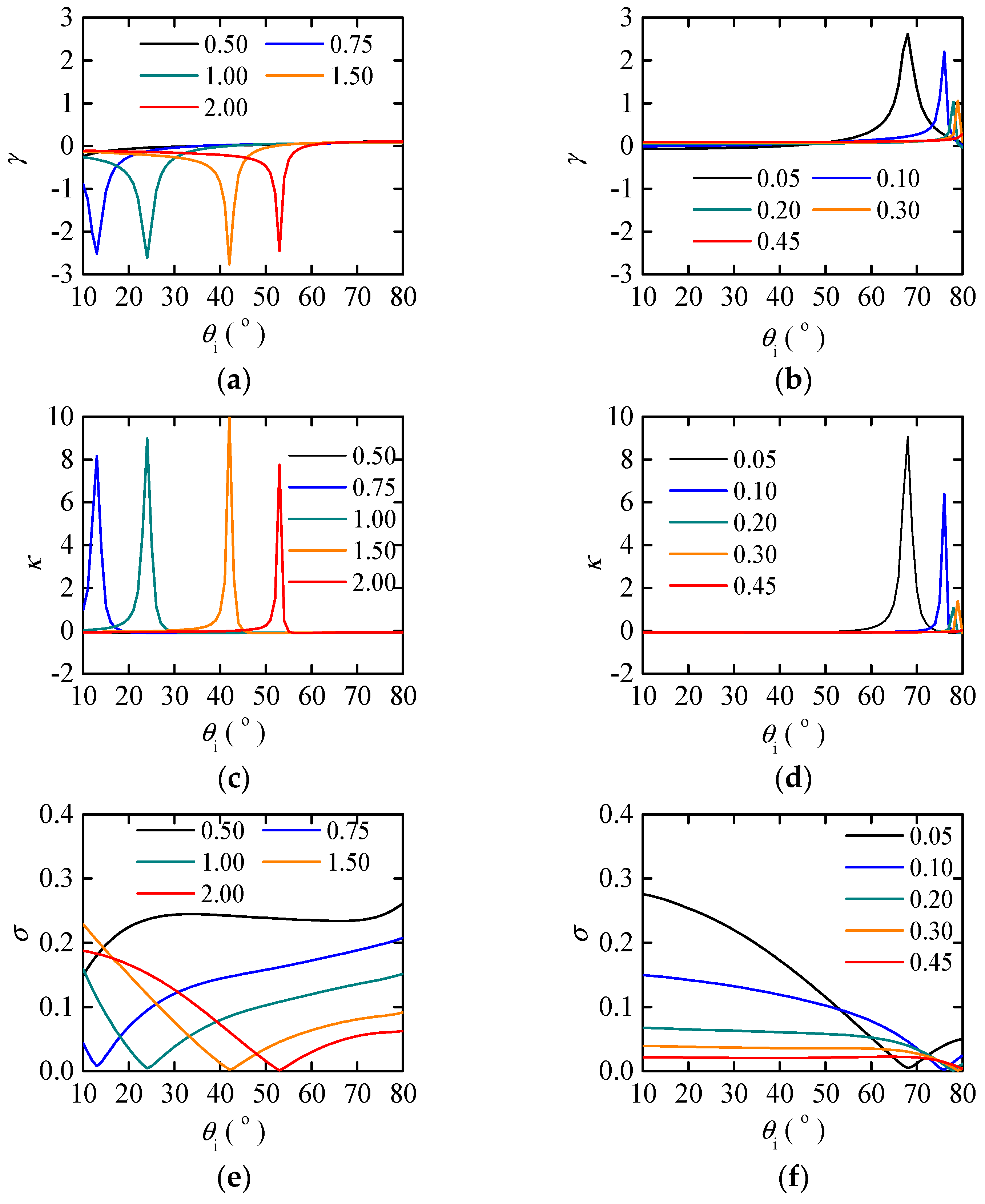
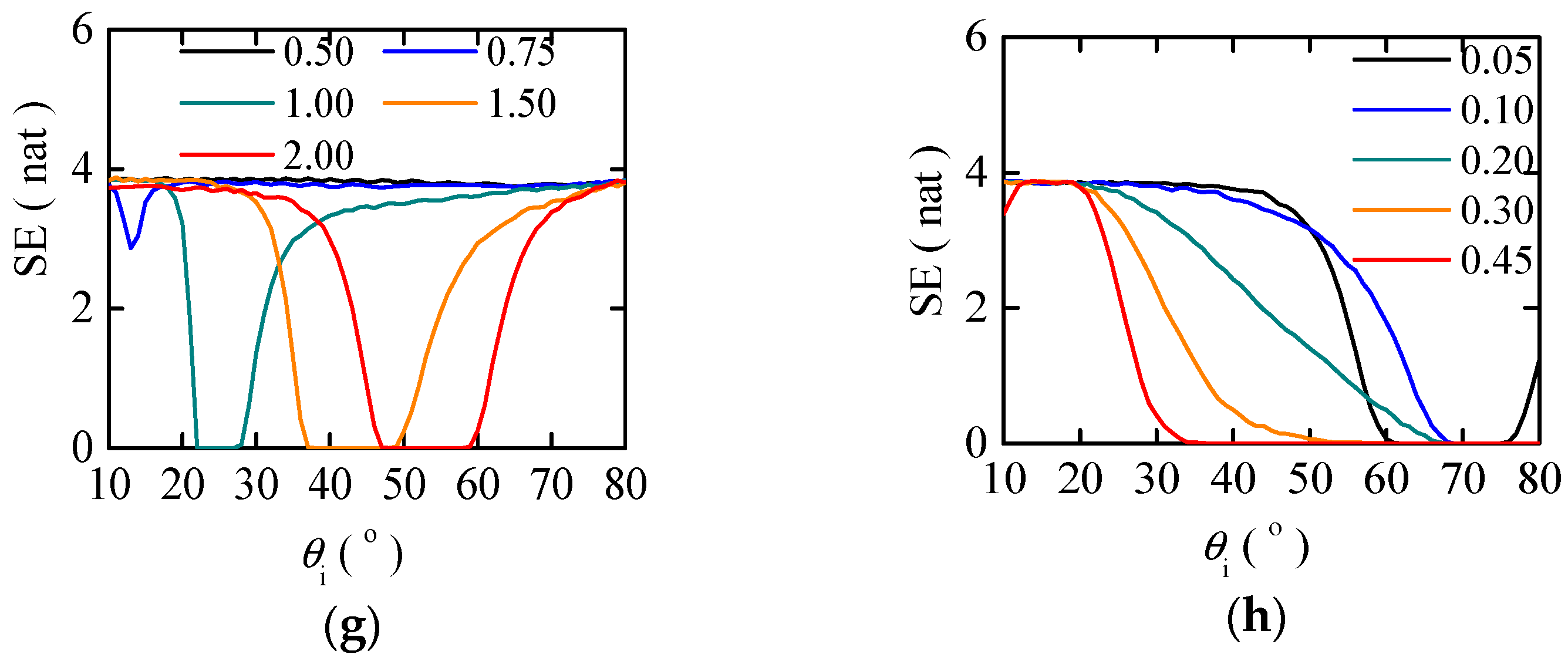
3.1. SA of Surface Condition
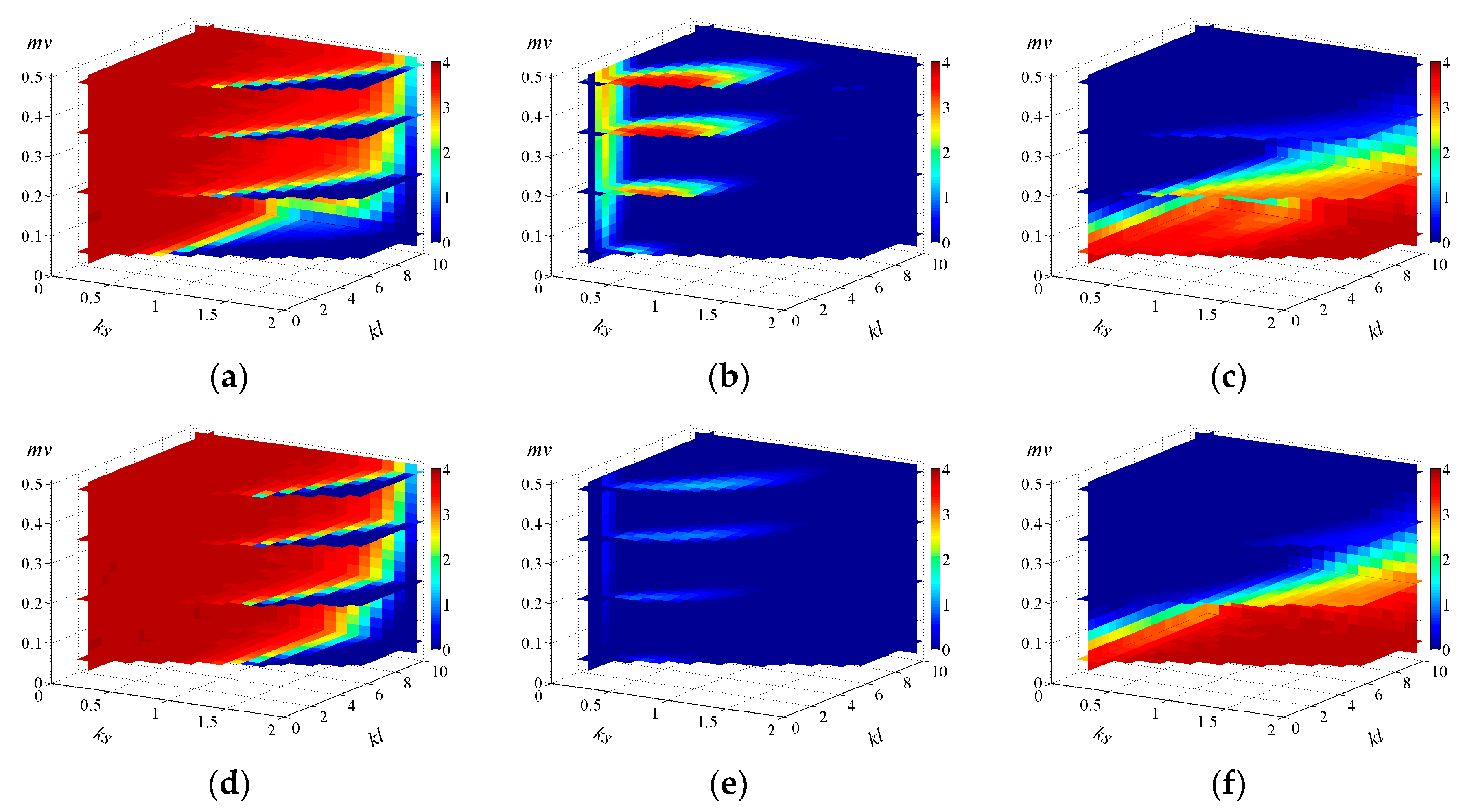
3.2. Sensitivity of Observation Configuration
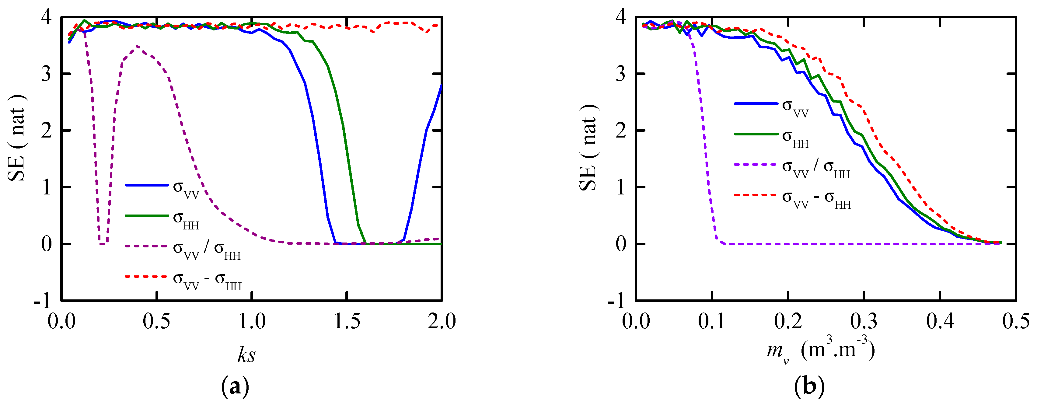
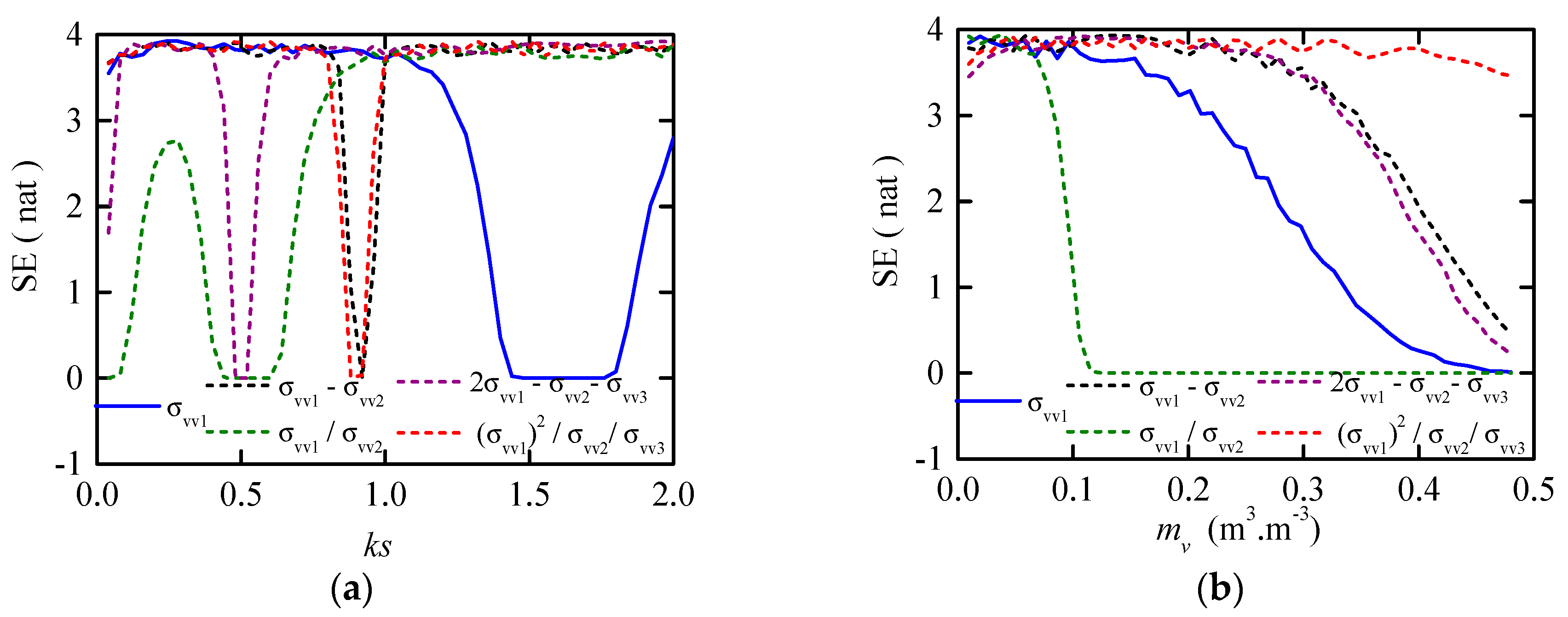
3.3. SA of Dual-Polarization and Multi-Angle
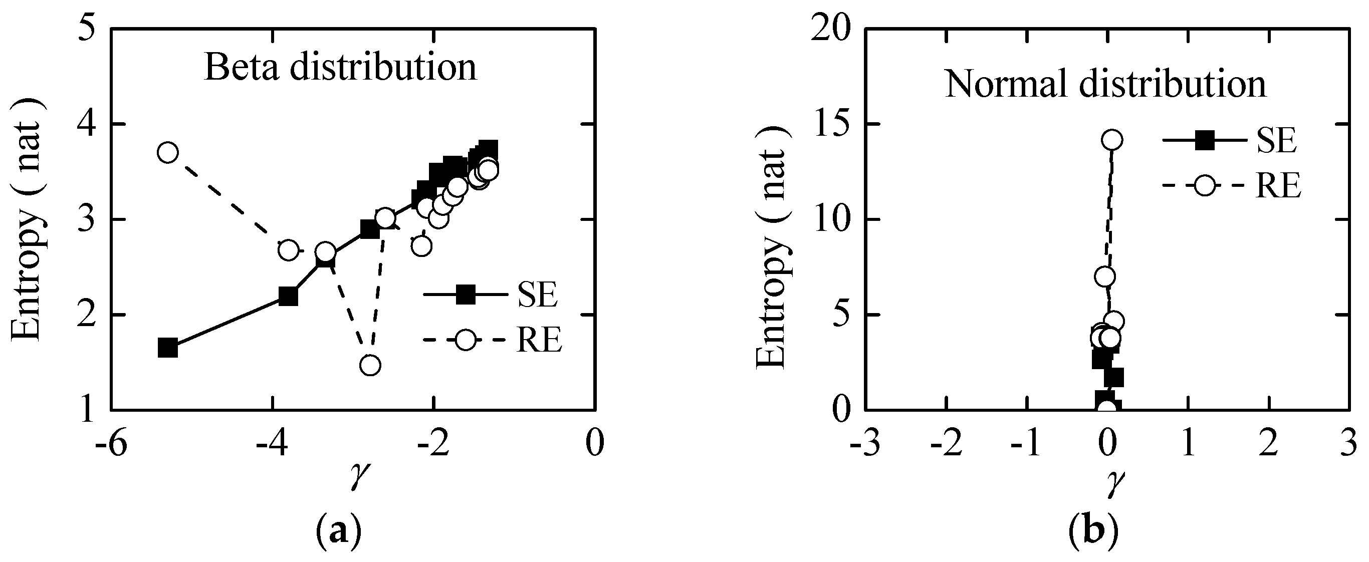
4. Discussion
5. Conclusions
Acknowledgments
Author Contributions
Conflicts of Interest
References
- Ulaby, F.T.; Long, D.G. Microwave Radar and Radiometric Remote Sensing; University of Michigan Press: Ann Arbor, MI, USA, 2014. [Google Scholar]
- Crosson, W.L.; Limaye, A.S.; Laymon, C.A. Parameter sensitivity of soil moisture retrievals from airborne L-band radiometer measurements in SMEX02. IEEE Trans. Geosci. Remote Sens. 2005, 43, 1517–1528. [Google Scholar] [CrossRef]
- Du, Y.; Ulaby, F.T.; Dobson, M.C. Sensitivity to soil moisture by active and passive microwave sensors. IEEE Trans. Geosci. Remote Sens. 2000, 38, 105–114. [Google Scholar] [CrossRef]
- Zribi, M.; Dechambre, M. A new empirical model to retrieve soil moisture and roughness from C-band radar data. Remote Sens. Environ. 2003, 84, 42–52. [Google Scholar] [CrossRef]
- Verhoest, N.E.; Lievens, H.; Wagner, W.; Álvarez-Mozos, J.; Moran, M.S.; Mattia, F. On the soil roughness parameterization problem in soil moisture retrieval of bare surfaces from synthetic aperture radar. Sensors 2008, 8, 4213–4248. [Google Scholar] [CrossRef] [PubMed]
- Lievens, H.; Verhoest, N.E.; De Keyser, E.; Vernieuwe, H.; Matgen, P.; Álvarez-Mozos, J.; De Baets, B. Effective roughness modeling as a tool for soil moisture retrieval from C-and L-band SAR. Hydrol. Earth Syst. Sci. 2011, 15, 151–162. [Google Scholar] [CrossRef]
- Zribi, M.; Gorrab, A.; Baghdadi, N. A new soil roughness parameter for the modelling of radar backscattering over bare soil. Remote Sens. Environ. 2014, 152, 62–73. [Google Scholar] [CrossRef]
- Bindlish, R.; Jackson, T.J.; Wood, E.; Gao, H.; Starks, P.; Bosch, D.; Lakshmi, V. Soil moisture estimates from TRMM Microwave Imager observations over the Southern United States. Remote Sens. Environ. 2003, 85, 507–515. [Google Scholar] [CrossRef]
- Chen, K.S.; Yen, S.K.; Huang, W.P. A simple-model for retrieving bare soil-moisture from radar-scattering coefficients. Remote Sens. Environ. 1995, 54, 121–126. [Google Scholar] [CrossRef]
- Mao, K.B.; Tang, H.J.; Zhang, L.X.; Li, M.C.; Guo, Y.; Zhao, D.Z. A method for retrieving soil moisture in Tibet region by utilizing microwave index from TRMM/TMI data. Int. J. Remote Sens. 2008, 29, 2903–2923. [Google Scholar] [CrossRef]
- Brogioni, M.; Pettinato, S.; Macelloni, G.; Paloscia, S.; Pampaloni, P.; Pierdicca, N.; Ticconi, F. Sensitivity of bistatic scattering to soil moisture and surface roughness of bare soils. Int. J. Remote Sens. 2010, 31, 4227–4255. [Google Scholar] [CrossRef]
- Saltelli, A.; Ratto, M.; Andres, T.; Campolongo, F.; Cariboni, J.; Gatelli, D.; Saisana, M.; Tarantola, S. Global Sensitivity Analysis: The Primer; John Wiley & Sons: West Sussex, UK, 2008. [Google Scholar]
- Wagner, S. Global sensitivity analysis of predictor models in soft- ware engineering. In Proceedings of the International Workshop on Predictor Models in Software Engineering, Minneapolis, MN, USA, 20–26 May 2007; p. 3. [Google Scholar]
- Petropoulos, G.; Srivastava, P.K. (Eds.) Sensitivity Analysis in Earth Observation Modelling; Elsevier: Oxford, UK, 2016. [Google Scholar]
- Ma, C.F.; Li, X.; Wang, S.G. A global sensitivity analysis of soil parameters associated with backscattering using the advanced integral equation model. IEEE Trans. Geosci. Remote Sens. 2015, 53, 5613–5623. [Google Scholar]
- McNairn, H.; Jackson, T.J.; Wiseman, G.; Belair, S.; Berg, A.; Bullock, P.; Colliander, A.; Cosh, M.H.; Kim, S.B.; Magagi, R.; et al. The soil moisture active passive validation experiment 2012 (SMAPVEX12): Prelaunch calibration and validation of the SMAP soil moisture algorithms. IEEE Trans. Geosci. Remote Sens. 2015, 53, 2784–2801. [Google Scholar] [CrossRef]
- Wang, J.; Li, X.; Lu, L.; Fang, F. Parameter sensitivity analysis of crop growth models based on the extended Fourier amplitude sensitivity test method. Environ. Model. Softw. 2013, 48, 171–182. [Google Scholar] [CrossRef]
- Estrada, V.; Diaz, M.S. Global sensitivity analysis in the development of first principle-based eutrophication models. Environ. Model. Softw. 2010, 25, 1539–1551. [Google Scholar] [CrossRef]
- Li, D.; Jin, R.; Zhou, J.; Kang, J. Analysis and reduction of the uncertainties in soil moisture estimation with the L-MEB model using EFAST and ensemble retrieval. IEEE Geosci. Remote Sens. Lett. 2015, 12, 1337–1341. [Google Scholar]
- Lentini, N.E.; Hackett, E.E. Global sensitivity of parabolic equation radar wave propagation simulation to sea state and atmospheric refractivity structure. Radio Sci. 2015, 50, 1027–1049. [Google Scholar] [CrossRef]
- Neelam, M.; Mohanty, B.P. Global sensitivity analysis of the radiative transfer model. Water Resour. Res. 2015, 51, 2428–2443. [Google Scholar] [CrossRef]
- Sobol, I.M. Sensitivity estimates for nonlinear mathematical models. Math. Model. Comput. Exp. 1993, 1, 407–414. [Google Scholar]
- Sudret, B. Global sensitivity analysis using polynomial chaos expansions. Reliab. Eng. Syst. Saf. 2008, 93, 964–979. [Google Scholar] [CrossRef]
- Saltelli, A.; Sobol, I.M. About the use of rank transformation in sensitivity of model output. Reliab. Eng. Syst. Saf. 1995, 50, 225–239. [Google Scholar]
- Saltelli, A.; Annoni, P. How to avoid a perfunctory sensitivity analysis. Environ. Model. Softw. 2010, 25, 1508–1517. [Google Scholar] [CrossRef]
- Shannon, C.E. A mathematical theory of communication. In ACM SIGMOBILE Mobile Computing and Communications Review; ACM: New York, NY, USA, 2001; Volume 5, pp. 3–55. [Google Scholar]
- Chen, K.S.; Wu, T.D.; Tsang, L.; Li, Q.; Shi, J.C.; Fung, A.K. Emission of rough surfaces calculated by the integral equation method with comparison to three-dimensional moment method simulations. IEEE Trans. Geosci. Remote Sens. 2003, 41, 90–101. [Google Scholar] [CrossRef]
- Wu, T.D.; Chen, K.S.; Shi, J.C.; Lee, H.W.; Fung, A.K. A study of AIEM Model for Bistatic Scattering from Randomly Surfaces. IEEE Trans. Geosci. Remote Sens. 2008, 46, 2584–2598. [Google Scholar]
- Chen, K.L.; Chen, K.S.; Li, Z.L.; Liu, Y. Extension and validation of an advanced integral equation model for bistatic scattering from rough surfaces. Prog. Electromagn. Res. 2015, 152, 59–76. [Google Scholar] [CrossRef]
- Dobson, M.C.; Ulaby, F.T.; Hallikainen, M.T.; El-Rayes, M.A. Microwave dielectric behavior of wet soil—Part II. Dielectric mixing models. IEEE Trans. Geosci. Remote Sens. 1985, 1, 35–46. [Google Scholar] [CrossRef]
- Peplinski, N.R.; Ulaby, F.T.; Dobson, M.C. Dielectric-properties of soils in the 0.3–1.3-GHz range. IEEE Trans. Geosci. Remote Sens. 1995, 33, 803–807. [Google Scholar] [CrossRef]
- Chen, K.S.; Wu, T.D.; Shi, J.C. A model- based inversion of rough surface parameters from radar measurements. J. Electromagn. Waves Appl. 2001, 15, 173–200. [Google Scholar] [CrossRef]
- Rényi, A. On measures of entropy and information. In Proceedings of the Fourth Berkeley Symposium on Mathematical Statistics and Probability, Berkeley, CA, USA, 20 June–30 July 1960; Volume 1, pp. 547–561. [Google Scholar]
- Liu, H.; Chen, W.; Sudjianto, A. Relative entropy based method for probabilistic sensitivity analysis in engineering design. J. Mech. Des. 2006, 128, 326–336. [Google Scholar] [CrossRef]
- Ziviani, A.; Gomes, A.T.A.; Monsores, M.L.; Rodrigues, P.S. Network anomaly detection using nonextensive entropy. IEEE Commun. Lett. 2007, 11, 1034–1036. [Google Scholar] [CrossRef]
- Phillips, S.J.; Dudík, M.; Schapire, R.E. A maximum entropy approach to species distribution modeling. In Proceedings of the Twenty-First International Conference on Machine Learning, Banff, AB, Canada, 4–8 July 2004; ACM: New York, NY, USA, 2004; p. 83. [Google Scholar]
- Parzen, E. On the estimation of a probability density function and the mode. Ann. Math. Stat. 1962, 33, 1065–1076. [Google Scholar] [CrossRef]


| Parameters | Range | ||
|---|---|---|---|
| Surface Parameter | ks | Normalized root mean surfaces height | 0.01~2 |
| kl | Normalized correlation length | 0.01~10 | |
| mv | Moisture content (m3m−3) | 0.01~0.45 | |
| Radar Parameter | θi | Incident angle | 10°~70° |
| θs | Scattering angle | =θi | |
| φs | Scattering azimuthal angle | 180° | |
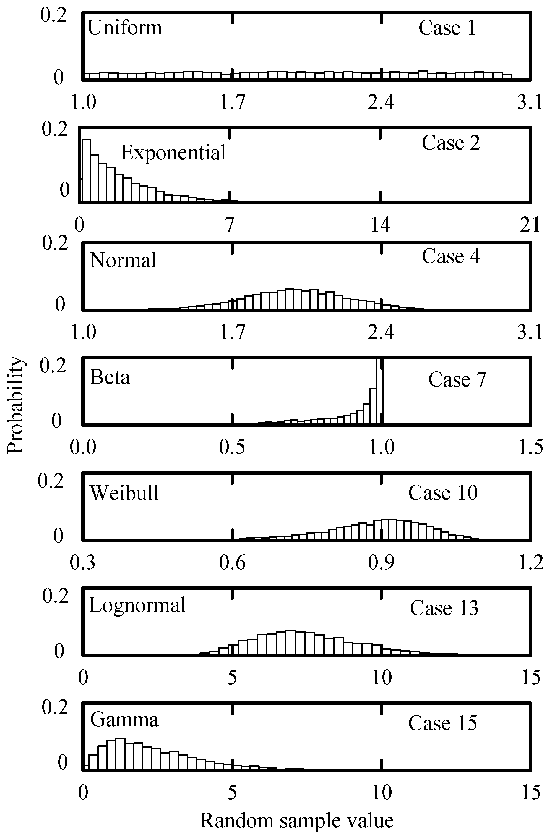
| Distribution | Equation 1 | Number | Parameters | SE (nat) | RE (nat) | |||
|---|---|---|---|---|---|---|---|---|
| Uniform | Case 1 | 0.01 | −1.18 | 0.57 | 3.75 | 3.76 | ||
| Exponential | Case 2 | 1.90 | 5.59 | 1.99 | 3.42 | 3.28 | ||
| Normal | Case 3 | −0.01 | 0 | 0.13 | 3.88 | 3.78 | ||
| Case 4 | −0.02 | 0.17 | 0.25 | 3.90 | 3.76 | |||
| Case 5 | 0.00 | −0.03 | 1.25 | 3.88 | 3.77 | |||
| Beta | 2 | Case 6 | −3.30 | 11.86 | 0.14 | 1.47 | −0.23 | |
| Case 7 | −2.03 | 3.8 | 0.18 | 2.66 | 1.77 | |||
| Case 8 | −0.59 | −0.55 | 0.23 | 3.77 | 3.67 | |||
| Weibull | Case 9 | 0.61 | 0.21 | 0.33 | 3.90 | 3.74 | ||
| Case 10 | −0.61 | 0.45 | 0.11 | 3.90 | 3.72 | |||
| Case 11 | −0.84 | 1.14 | 0.06 | 3.84 | 3.73 | |||
| Lognormal | Case 12 | 0.18 | 0.08 | 0.47 | 3.88 | 3.78 | ||
| Case 13 | 0.86 | 1.33 | 1.96 | 3.86 | 3.72 | |||
| Case 14 | 1.56 | 3.45 | 4.38 | 3.63 | 3.56 | |||
| Gamma | Case 15 | 1.33 | 2.47 | 0.35 | 3.69 | 3.58 | ||
| Case 16 | 1.36 | 2.7 | 1.76 | 3.64 | 3.61 |
© 2018 by the authors. Licensee MDPI, Basel, Switzerland. This article is an open access article distributed under the terms and conditions of the Creative Commons Attribution (CC BY) license (http://creativecommons.org/licenses/by/4.0/).
Share and Cite
Liu, Y.; Chen, K.-S. An Information Entropy-Based Sensitivity Analysis of Radar Sensing of Rough Surface. Remote Sens. 2018, 10, 286. https://doi.org/10.3390/rs10020286
Liu Y, Chen K-S. An Information Entropy-Based Sensitivity Analysis of Radar Sensing of Rough Surface. Remote Sensing. 2018; 10(2):286. https://doi.org/10.3390/rs10020286
Chicago/Turabian StyleLiu, Yu, and Kun-Shan Chen. 2018. "An Information Entropy-Based Sensitivity Analysis of Radar Sensing of Rough Surface" Remote Sensing 10, no. 2: 286. https://doi.org/10.3390/rs10020286
APA StyleLiu, Y., & Chen, K.-S. (2018). An Information Entropy-Based Sensitivity Analysis of Radar Sensing of Rough Surface. Remote Sensing, 10(2), 286. https://doi.org/10.3390/rs10020286