The Influence of Sub-Block Position on Performing Integrated Sensor Orientation Using In Situ Camera Calibration and Lidar Control Points

Abstract

The accuracy of photogrammetric and Lidar dataset integration is dependent on the quality of a group of parameters that models accurately the conditions of the system at the moment of the survey. In this sense, this paper aims to study the effect of the sub-block position in the entire image block to estimate the interior orientation parameters (IOP) in flight conditions to be used in integrated sensor orientation (ISO). For this purpose, five sub-blocks were extracted in different regions of the entire block. Then, in situ camera calibrations were performed using sub-blocks and sets of Lidar control points (LCPs), computed by a three planes’ intersection extracted from the Lidar point cloud on building roofs. The ISO experiments were performed using IOPs from in situ calibrations, the entire image block, and the exterior orientation parameters (EOP) from the direct sensor orientation (DSO). Analysis of the results obtained from the ISO experiments performed show that the IOP from the sub-block positioned at the center of the entire image block can be recommended.

1. Introduction

The integration of Lidar and photogrammetric datasets has been an important research subject aiming to increase the automation of geoinformation extraction in photogrammetric mapping procedures. According to Rönnholm [1], it is expected that the integration of such technologies will become a simple and common procedure applied in automatic object recognition, vegetation classification, land use and 3D modeling. Traditionally, indirect and direct georeferencing have been the procedures used to perform this integration by the estimation of the exterior orientation parameters (EOP) of the imagery photogrammetric block.

Indirect georeferencing requires geometric primitives on the ground to define the mapping frame and fix the 3D photogrammetric intersection. Using Lidar data as a source of positional information, methods to extract geometric primitives (points, lines and areas) are required, since the Lidar dataset does not show, directly, such primitives. Several studies have been conducted on this thematic. Delara et al. [2] performed research to extract Lidar control points (LCPs) from Lidar intensity images for application in aerial triangulation using a low-cost digital camera. Habib et al. [3] and Habib et al. [4] implemented registration methods between Lidar and photogrammetric data using liner features and 3D similarity transformation. Csanyi and Toth [5] conducted research to develop an optimal ground-control target to improve the accuracy of Lidar data in mapping projects. Mitishita et al. [6] proposed an approach to extract the centroid of building roofs from Lidar point clouds. In [7], LCPs were used in the aerial triangulation process of a large photogrammetric block of analog aerial photographs. According to the authors, the mapping achieved national standard cartographic accuracy for the 1:50,000 scale mapping. Ju et al. [8] developed a hybrid two-step method for robust Lidar/optical imagery registration, taking advantage of feature, intensity, and frequency-based methods. Gneeniss [9] conducted research to integrate photogrammetric dense tie points and Lidar cloud using a robust 3D least-squares surface-matching algorithm. Li et al. [10] proposed an approach using sand ridges as primitives to solve the registration problem between Lidar and imagery in regions where ground-control points (GCPs) are not available, for instance, desert areas.

Direct sensor orientation is another approach used in simultaneous photogrammetric and Lidar surveys. This procedure can automatically acquire the Lidar and imagery datasets in the same mapping frame by global navigation satellite system and inertial measurement unit (GNSS/IMU) systems. However, the accuracies of the integration of the photogrammetric and Lidar datasets are dependent on the quality of parameters that models accurately the systems at the same time as the survey. Gneeniss et al. [11] proposed a methodology to perform camera self-calibration using LCPs in the bundle-block adjustment (BBA). The approach provided an efficient and cost-effective alternative for in-flight camera calibration. Scott et al. [12] developed a generic calibration algorithm to calibrate a sensor system consisting of 2D Lidars and cameras, where the sensor fields-of-view (FoVs) are not required to overlap. According to the authors, it is impossible to overstate the importance of good calibration in Lidar–camera systems. Dhall et al. [13] presented an approach to find accurate 3D rigid-body transformation for the calibration of low-density Lidar and photogrammetry datasets. The main advantage of the method is estimating the transformation parameters with a smaller number of points and correct correspondences.

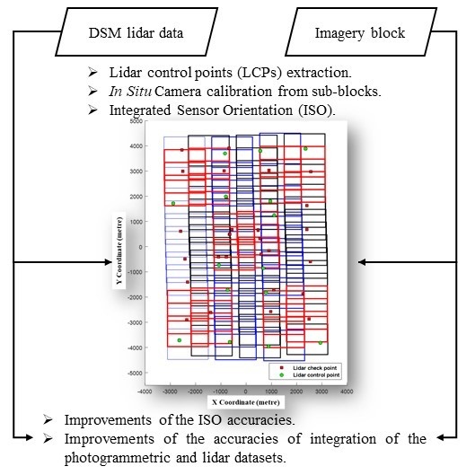
In this sense, using Lidar control points in integrated sensor orientation (ISO) can improve the quality of the integration of the photogrammetric and Lidar datasets by the refinement of the EOP. However, to perform the ISO over the entire photogrammetric block, some requirements must be considered. Firstly, the block configuration should have enough forward and side overlap areas with a minimum number of tie points located in the overlapping areas of the stereo pairs (Von Gruber positions); accurate interior orientation parameters (IOP) values; and finally, the standard deviations of the direct EOP values [14].

The use of a sub-block of images to perform the in situ camera calibration was proposed by [15] for improving the performance of ISO, using three signalized control points (2 horizontal/vertical and 1 vertical) from a GNSS survey. The results showed an increase in the horizontal and vertical accuracies when compared to the use of an IOP provided by the company. Mitishita et al. [16] performed an empirical study of the importance of the in situ camera calibration in ISO to increase the accuracies of the photogrammetric and Lidar datasets’ integration when it was compared with ISO using IOP from the manufacturer.

In practical mapping flight missions with large photogrammetric blocks, conducting a GNSS survey in the entire block is very expensive. In addition, the distribution of GCPs is a key element for achieving high ISO accuracy. Besides, access in conflict areas is not possible or is restricted. So, this paper proposes an alternative approach to estimate the IOP values derived from the sub-block, using the benefit of the complementarity of Lidar and photogrammetry datasets in order to avoid a GNSS survey.

The main points to be investigated in this study are: (i) the position of a small sub-block of images on the entire image block is important for estimating IOP values by in situ camera calibration using LCPs; and (ii) the result obtained from the in situ camera calibration using a sub-block can be used to improve the accuracies of the ISO using the entire block. Additionally, this study can contribute to improving the accuracy of integration of the photogrammetric and Lidar datasets by in situ camera calibration and ISO. Moreover, additional effort in-flight and data processing can be reduced.

The sections are organised as follows: first, materials and methodology are shown and discussed. This section gives detailed descriptions of imagery and Lidar datasets used to perform the experiments. Then, the proposed methodology is explained in three main steps. The subsequent section shows the results and discusses the experiments. Finally, conclusions and recommendations for future work are given.

2. Materials and Methods

The TRIMBLE digital aerial camera AIC PRO +65, mounted with HR Digaron-W 50 f/1.4 lens was used in this study. The camera CCD sensor has 60 million effective pixels (8984 × 6732 pixels), dimension of 53.9 mm × 40.4 mm, and the pixel size is 6 µm. The TRIMBLE camera was connected to the Optech Airborne Laser Scanner ALTM Pegasus HD500 to perform airborne Lidar and imagery surveys simultaneously. The camera was installed on the same platform as the Lidar system. It was connected to the Lidar system through an RS232 serial cable to record the images taken along the Lidar GNSS/INS trajectory in order to compute the position and orientation of the camera. The Optech Airborne Laser Scanner Pegasus_HD500 has an applanix inertial measurement unit (IMU) POS AV 510. The IMU absolute accuracies (RMS)—position <0.1 m; roll and pitch <0.005 deg; yaw <0.008 deg.

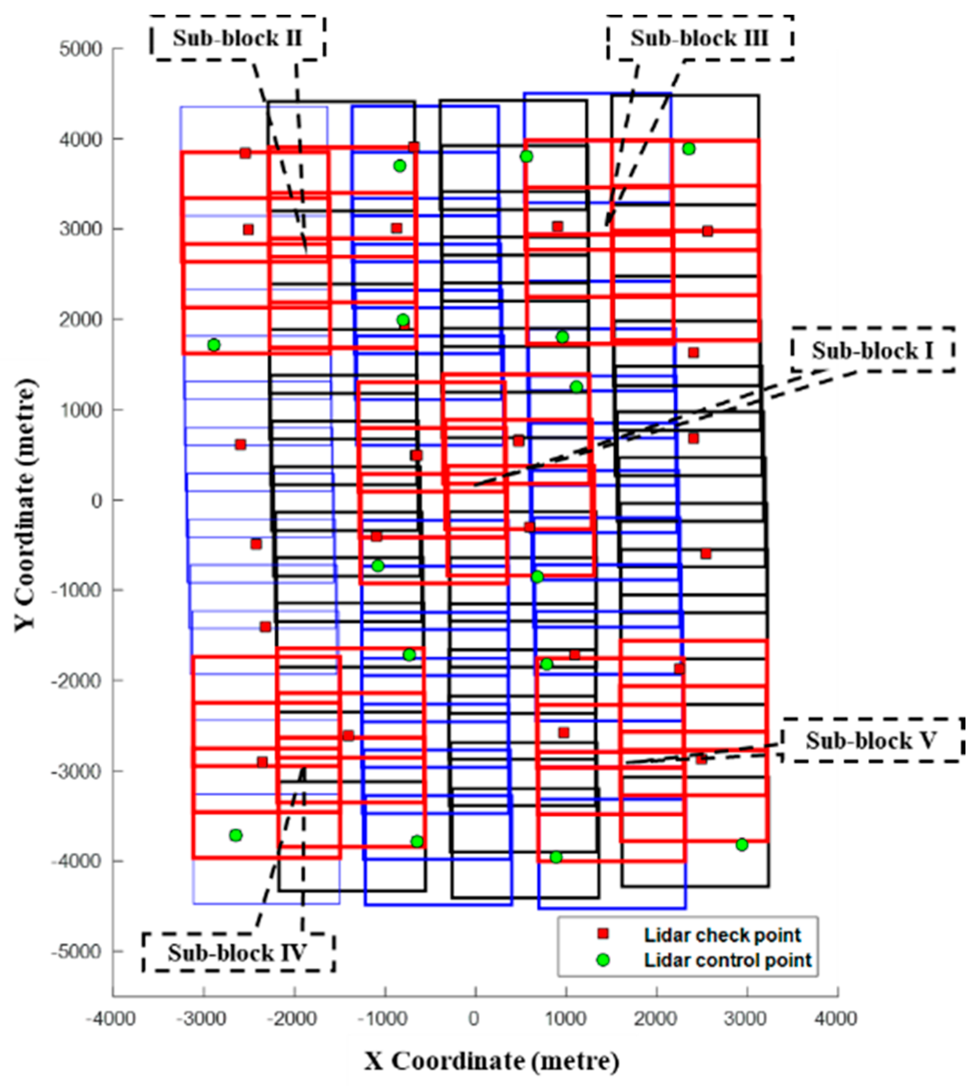
A photogrammetric image block was acquired on August 2012. The block has six strips, taken in opposite directions (approximately north-to-south and south-to-north) with around 45% of lateral overlap. Each strip has 16 images, acquired with nearly 60% forward overlap. Figure 1 shows the layout of the imagery block and the five sub-blocks labelled from I to V. For the applied flight height of approximately 1600 m, the image pixel resolution on the ground (GSD) resulted close to 0.18 m. A suburban area of approximately 57 km² in size, of the city Curitiba (state of Paraná, Brazil) was covered by the images. Simultaneous to the photogrammetric survey, the individual Lidar strips were collected with a mean point density of 5 points/m² (nearly 0.25 m point spacing). According to the sensor and flight specifications, 0.18 m horizontal and 0.15 m vertical accuracies are expected for the acquired Lidar data.

2.1. Lidar Control Point (LCP) Extraction

LCPs are considered in this study as the ground reference to fix the Lidar and photogrammetric datasets on the same mapping frame. They are used as control or check points to perform the experiments of the in situ camera calibration and integrated sensor orientation.

Many approaches have been developed to extract image point features from Lidar point cloud or Lidar intensity images. Usually, point features are extracted after defining existing geometric shapes such as buildings’ corners or ridge roof corners. Gneeniss [9] presented a complete background about different methods to extract specific features. The approach performed in this research was focused on point-feature extraction by the intersection of three building roof planes. According to Costa et al. [17], the method is composed of four main steps: filtering Lidar points on the building of roofs; roof building planes’ extraction; roof building planes’ modelling; intersection of three planes (LCP characterization). The first step is undertaken by identification of the residential areas, which must contain one or more buildings with roofs defined by three or more planes. Then, Lidar points are classified on the building roofs and are divided into specific planes. Finally, the 3D coordinates of the LCP is calculated by the intersection of three roof planes of one building.

The modeling of the building roof planes was based on the least squares adjustment using the context of normal vectors of the surrounding points. Outliers were detected by the analysis of residuals in the three components (X, Y, Z) simultaneously. To perform this study, 37 Lidar-derived points (LCPs) were extracted along the entire block to be used as control or check points.

2.2. In Situ Camera Calibration

The in situ calibration process aims to estimate the IOP of the TRIMBLE camera in the conditions of the aerial survey. In contrast to current techniques, the new method focuses on using Lidar-derived control points and small sub-blocks of images extracted from the entire block. Besides this, it is not necessary to undertake a calibration test field. The calibration experiments were performed using five small sub-blocks labelled I to V. Each sub-block had six images distributed in two strips (three images in each strip).

Using the collinearity equations Equations (1) to (5) from the Brown–Conrady model [18] and least-squares bundle block adjustment (BBA) [19], the theoretical collinearity condition among image point, the position of the camera station and object point can be in practice recovered by additional parameters related to lens distortions, coordinates of principal point (i.e., the point in image plane closest to the projection center) and the sensor distortions. Mitishita et al. [19], Gneeniss [9] and Gneeniss et al. [11] gave details about the main steps used to perform the in situ calibration using different digital cameras.

The aforementioned dependencies can be described as follows:

$$x -x_o=-f·\frac{m_{11}\left(X-X_o\right)+m_{12}\left(Y-Y_o\right)+m_{13}\left(Z-Z_o\right)}{m_{31}\left(X-X_o\right)+m_{32}\left(Y-Y_o\right)+m_{33}\left(Z-Z_o\right)}+\Delta x,$$

(1)

$$y-y_o=-f·\frac{m_{21}\left(X-X_o\right)+m_{22}\left(Y-Y_o\right)+m_{23}\left(Z-Z_o\right)}{m_{31}\left(X-X_o\right)+m_{32}\left(Y-Y_o\right)+m_{33}\left(Z-Z_o\right)}+\Delta y,$$

(2)

$$\begin{gathered} \Delta x=\left(K_1{r}^2+K_2{r}^4+K_3{r}^6\right)\left(x-x_o\right)+P_1[r^2+2{\left(x-x_o\right)}^2] \\ +2P_2\left(x-x_o\right)\left(y-y_o\right)+b_1\left(x-x_o\right)+b_2\left(y-y_o\right), \end{gathered}$$

(3)

$$\begin{gathered} \Delta y=\left(K_1{r}^2+K_2{r}^4+K_3{r}^6\right)\left(y-y_o\right)+2P_1\left(x-x_o\right)\left(y-y_o\right) \\ +P_2[r^2+2{\left(y-y_o\right)}^2]+b_1\left(y-y_o\right), \end{gathered}$$

(4)

with

$$r^2={\left(x-x_o\right)}^2+{\left(y-y_o\right)}^2,$$

(5)

where ($x,y$) are the image coordinates in millimeters; $f$ is the focal length in millimeters; ($X, Y, Z$) are the object point coordinates usually given in meters in the mapping reference system (i.e., Earth-fixed coordinate system, in the case UTM); ($X_o,Y_o,Z_o)$ are the coordinates of the camera station at the time of exposure, usually given in meters in the mapping reference system; ($x_o,y_o)$ are principal point coordinates of the camera in millimeters; ($\Delta x,\Delta y)$ are the correction terms due to lens and sensor frame systematic errors, radial symmetric ($K_1,K_2,K_3$), decentering distortion coefficients ($P_1,P_2$) and affinity parameters ($b_1,b_2$) of the camera; and m_ij are the rotation matrix elements of the camera orientation angles in the mapping-reference system.

According to Mitishita et al. [15], three LCPS that are not aligned are required to perform the in situ calibration process considering the sub-block dimension. They were extracted from the Lidar point cloud using the methodology described in [17]. Approximately 30 tie points, close to Von Gruber regions, were measured using the Leica Photogrammetry Suite application (LPS) 2011. Additionally, the direct measurement of the position and orientation of the camera by GNSS/IMU sensors were also used to perform the in situ self-calibration. The nominal standard deviations for the direct measurement were introduced in the bundle adjustment process by weight constraints (position <0.1 m; roll and pitch <0.005 deg; yaw <0.008 deg).

Reference values to analyze the obtained results from the sub-block calibration experiments were acquired by the in situ calibration using the entire block. It was expected that IOP values, obtained from the entire block, would achieve better results for object space coordinates. However, as remarked in [9], four full LCPs, positioned at the corner of block, were recommended to perform this calibration.

2.3. Integrated Sensor Orientation (ISO)

The ISO was performed to refine the values of the EOP from direct sensor orientation [20]. The assumption of this research is that ISO using IOP values, estimated by in situ sub-block calibration, can improve the accuracies of the integration of Lidar and photogrammetric datasets.

The entire photogrammetric block without control points was used to perform five ISO experiments using the IOPs from the in situ sub-block calibrations.

As already mentioned, reference values to verify the accuracies obtained from the five ISO experiments are acquired by an ISO experiment using the entire image block with four LCPs (positioned on the corners of the block). Together with this ISO experiment, a new set of IOP, considering the entire image block, was also estimated.

All experiments used 334 tie points over the overlap areas and the measurements performed by automatic procedures in LPS software. The direct EOP measured from GNSS/INS sensors were included in the BBA as additional observations by weight constraint.

The horizontal and vertical accuracies of the ISO experiments were assessed using the independent LCP check-point discrepancies. For the horizontal accuracy, two GSD (36 cm) were used as the limit value. The vertical accuracy considered the value of the 3D photogrammetric intersection based on the average flight height (1600 m), the average baseline (508 m), the image-measurement precision (0.003 m), and the mean focal length from the calibrations (51.7 mm). Then, using the mathematical equation shown in [21], the expected vertical accuracy is close to 41 cm.

3. Results and Discussion

3.1. Lidar Control Point (LCP) Extraction

Thirty-seven LCPs were extracted from the Lidar point cloud using the methodology described in Section 2.1. They were used as control or check points to perform the experiments of the in situ camera calibration and ISO.

The approach developed to extract the LCPs requires high-density Lidar point over the building roof regions. Additionally, the surface of the roofs should be smooth to obtain precision plane adjustments. However, if the conditions described are not fulfilled, the approach can still be applied but more iterations are required and lower accuracies of 3D coordinates of the LCPs are expected. In this study, the 37 LCPs were extracted from medium density-point cloud (close to 4 points/m²).

In this study, there was no ground truth used to check the horizontal and vertical accuracies of the LCPs’ 3D coordinates. According to [22], the horizontal position accuracy of the points extracted from the Lidar point cloud can vary from 0.1 m to 1.0 m. Considering the nominal Lidar 3D coordinates precision (18 cm for X and Y coordinates and 15 cm for Z coordinates), the value of 0.36 cm (two σ—Standard deviation) was empirically assumed for the LCP horizontal precision; and for the vertical precision, the value of 15 cm was assumed. The assessment of the 3D coordinates of some LCPs is done by the residual analyses from the in situ camera calibration experiments described in the next section.

3.2. In Situ Camera Calibration

The in-house bundle block adjustment program (calibration and aerial triangulation) was used to perform the in situ camera calibration experiments. Based on the variance-covariance matrix from the adjustment, a parameter was considered significant when its standard deviation was at least 10 times smaller than the parameter magnitude [23].

All in situ camera calibration experiments used the following measurement precisions: 0.003 mm (half of a pixel) for x and y image coordinates; 36 cm for X and Y coordinates; and 15 cm for Z coordinates for the LCPs (Lidar 3D coordinates accuracies). For the direct EOPs, nominal values were adopted of 10 cm for positions and 0.005 arc degrees for Omega and Phi, and 0.008 arc degrees for Kappa, considering the results of the trajectory accuracies in post-processing position and orientation systems (POS).

Table 1. Main results of the residual analysis performed from in situ camera calibrations.

In Situ Calibration Experiments	Residuals in Image Coordinates (µm)		Residuals in Lidar Control Points Coordinates (cm)			Residuals in Camera Stations Coordinates (cm)			Residuals in Camera Stations Orientation (arcsec)
	Root-Mean-Square Error (RMSE) in x/y		RMSE in X/Y/Z			RMSE in Xs/Ys/Zs			RMSE in ω/φ/κ
Sub-block I	2.0	1.0	8.7	17.1	2.8	1.6	2.3	3.6	7.2	3.6	7.2
Sub-block II	1.0	1.0	22.1	22.4	2.9	2.3	2.3	2.1	7.2	7.2	18
Sub-block III	1.0	1.0	29.8	23.4	2.9	2.0	2.9	2.9	7.2	3.6	18
Sub-block IV	1.0	1.0	6.0	2.3	1.0	1.0	1.0	1.0	3.6	3.6	7.2
Sub-block V	1.0	1.0	12.6	18.2	2.9	2.0	1.5	2.0	3.6	3.6	10.8
Entire block	1.0	2.0	7.7	1.8	1.8	1.8	1.5	3.6	3.6	3.6	10.8

shows the results of the precision analysis of the in situ camera calibration experiments. The root-mean-square errors (RMSEs) of the measurement residuals were used to verify the results obtained from the five in situ camera calibrations. In all calibrations, the RMSE of the residuals of the image coordinates were smaller than a priori precisions (0.003 mm). In addition, the RMSE residuals from the direct measurement positions (X_s, Y_s, Z_s) and orientations (ω, φ, κ) of the sensor were smaller than a priori precisions. The RMSE residuals of the camera stations positions varied from 1.0 to 3.6 cm and the orientations from 0.001–0.005 arc degrees. The RMSE of the X-Y components from the LCPs residuals in the sub-block II, III were slightly bigger than the expected values. However, the precisions obtained were acceptable considering they are close to 36 cm (two standard deviations).

The results of the IOP from the in situ camera calibration experiments can be seen in

Table 2. Estimated interior orientation parameters (IOP) by in situ camera calibrations.

IOP Values	Sub-Block I	Sub-Block II	Sub-Block III	Sub-Block IV	Sub-Block V	Entire Block
f (mm)	51.658	51.635	51.685	51.657	51.670	51.665
σf (mm)	0.008	0.013	0.012	0.010	0.014	0.005
xo (mm)	0.100	0.100	0.098	0.099	0.100	0.101
σxo (mm)	0.002	0.003	0.002	0.002	0.003	0.000
yo (mm)	0.130	0.132	0.131	0.132	0.130	0.130
σyo (mm)	0.002	0.002	0.002	0.001	0.002	0.000
k1 (mm−2)	−1.385 × 10−5	−1.417 × 10−5	−1.458 × 10−5	−1.487 × 10−5	−1.417 × 10−5	−1.489 × 10−5
σk1 (mm−2)	4.245 × 10−7	4.161 × 10−7	3.748 × 10−7	3.229 × 10−7	5.102 × 10−7	1.845 × 10−7
k2 (mm−4)	3.250 × 10−9	3.591 × 10−9	3.987 × 10−9	4.316 × 10−9	3.613 × 10−9	4.689 × 10−9
σk2 (mm−4)	4.087 × 10−10	3.714 × 10−10	3.765 × 10−10	3.166 × 10−10	4.246 × 10−10	3.669 × 10−10
P1 (mm−1)	2.692 × 10−6	3.918 × 10−6	1.851 × 10−6	6.188 × 10−6	4.565 × 10−6	3.410 × 10−6
σP1 (mm−1)	1.698 × 10−6	2.184 × 10−6	2.061 × 10−6	1.474 × 10−6	1.858 × 10−6	2.698 × 10−7
P2 (mm−1)	5.749 × 10−6	5.158 × 10−6	6.241 × 10−6	5.251 × 10−6	5.584 × 10−6	5.464 × 10−6
σP2 (mm−1)	7.480 × 10−7	6.841 × 10−7	6.967 × 10−7	6.284 × 10−7	7.716 × 10−7	1.167 × 10−7

f = focal length; (x_o, y_o) = coordinates of principal point; (k₁, k₂, k₃) = radial lens distortion; (P₁, P₂) = decentering lens distortion; (σ) = Standard deviation.

. The IOP values from the five calibrations are compared among the IOP obtained from all calibrations. The principal point coordinates are equal in every calibration. The maximum x coordinate difference is observed between sub-block III and the entire block (close to 3 µm). For the y coordinate, the maximum difference value was 2 µm. However, the values of focal length, obtained from in situ calibration of the sub-block II and III, are significantly different from the others’ calibration. These variations can be related to some inaccuracies in the LCPs 3D coordinates or in the direct measurement of the camera station. The radial symmetric distortions, modeled by the parameters K₁ and K₂, are nearly the same for all sub-block in situ calibrations. The values of parameter K₃ were not considered because their standard deviations from the variance covariance matrix were greater than the accepted values. Due to the misalignment of the lens elements, the decentering lens distortions are different in all sub-blocks’ in situ calibrations, as can be seen in the values of the P₁ parameters.

3.3. Integrated Sensor Orientation (ISO)

The importance of the IOP, estimated under in-flight conditions, for performing the ISO procedure is evaluated in this study. Additionally, the influence of the location of the small sub-block in the entire image block for estimating the IOP by in situ calibration is evaluated. Five ISO experiments without control points using the entire image block and the IOP from five in situ sub-blocks calibrations were carried out. The positions of the five small images sub-blocks at the entire block are shown in Figure 1.

Using the 37 check points, the horizontal and vertical discrepancies were computed by comparison of 3D coordinates, obtained by 3D-photogrammetric intersection and three Lidar planes’ intersection.

Additional two ISO experiments with four LCPs, positioned at the corners’ block, were performed in order to acquire reference values to support the performed analyses. In the first, the in situ calibration was performed together to estimate IOP considering the entire image block. The second ISO experiment was performed using the IOP from the manufacturer’s certificate.

The ISO experiments used the following measurement precisions: 0.003 mm (half of a pixel) for x and y image coordinates; 36 cm for X and Y coordinates; and 15 cm for Z coordinates for the LCPs. The direct measurements of the camera stations (EOP values) for the first five experiments were weighted according to the precisions estimated by in situ calibrations (showed in Table 1). The others two ISO experiments at the camera stations (EOP values) were weighted according to GNSS/INS nominal precisions. The main results obtained in all the ISO experiments are shown in

Table 3. Main results of the residuals analyses of the seven integrated sensor orientation (ISO) experiments.

ISO Experiments	Residuals in Image Coordinates (µm)		Residuals in Camera Stations’ Coordinates (cm)			Residuals in Camera Stations’ Orientation (arcsec)
	RMSE in x/y		RMSE in Xs/Ys/Zs			RMSE in ω/φ/κ
Sub-block I	1.6	1.8	0.4	0.3	1.0	3.6	0.0	3.6
Sub-block II	1.5	1.8	0.4	0.5	0.4	3.6	3.6	7.2
Sub-block III	1.6	2.0	1.5	0.8	0.7	3.6	3.6	10.8
Sub-block IV	1.6	1.9	0.1	0.3	0.1	3.6	0.0	3.6
Sub-block V	1.5	1.8	0.4	0.3	0.4	0.0	0.0	3.6
Entire block in situ calibration	1.0	2.0	1.8	1.5	3.6	3.6	3.6	10.8
Entire block IOP manufacturer	3.0	4.0	79.5	73.5	6.0	183.6	198.0	57.6

and

Table 4. Results of the check point discrepancies from the ISO experiments.

Check Point Discrepancies
		DX	DY	DH	DZ
ISO Sub-block I	µ	10.6	11.0	41.6	6.0
	RMSE	34.5	33.8	48.3	23.5
	Max	73.3	107.4	119.5	55.4
ISO Sub-block II	µ	10.9	10.2	41.9	−68.8
	RMSE	34.7	34.0	48.6	72.6
	Max	71.9	106.7	118.9	−29.7
ISO Sub-block III	µ	10.6	11.7	40.5	63.5
	RMSE	32.5	34.7	47.5	68.4
	Max	70.7	109.2	121.2	143.9
ISO Sub-block IV	µ	10.5	10.7	41.1	−15.1
	RMSE	33.8	34.1	48.0	28.2
	Max	67.9	105.2	117.9	23.3
ISO Sub-block V	µ	10.4	11.1	41.1	42.0
	RMSE	34.3	33.6	48.0	48.0
	Max	70.9	106.9	119.2	79.21
ISO Entire block in situ calibration	µ	11.3	11.9	41.0	7.2
	RMSE	34.0	33.9	48.0	21.4
	Max	68.9	107.3	120.4	−1.3
ISO Entire block IOP Manufacturer	µ	3.3	23.9	55.3	113.0
	RMSE	42.8	45.4	62.4	127.6
	Max	105.3	92.9	119.8	218.6

µ = mean values of the discrepancies (cm); RMSE = root mean square error of the discrepancies (cm); Max = maximum discrepancy (cm); DH = horizontal discrepancy (cm).

.

Table 3 shows RMSEs of the measurement residuals obtained from all ISO experiments. Except for the ISO experiment using IOP from the manufacturer, the RMSEs computed by the residuals of the image coordinates were smaller than a priori precisions (0.003 mm). Additionally, the RMSE residuals from the direct measurement positions (X_s, Ys, Z_s) and orientations (ω, φ, κ) of the sensor were smaller than a priori precisions. The RMSE residuals of the camera stations’ positions vary from 1.0 cm to 3.6 cm and the orientations from 0.001–0.005 arc degrees.

Non-acceptable residuals in the direct measurements of the positions and orientation of sensor were achieved when a set of IOPs from the manufacturer was used in the ISO experiment. These results indicate that the nominal IOP do not have the same accuracies as those estimated in flight conditions.

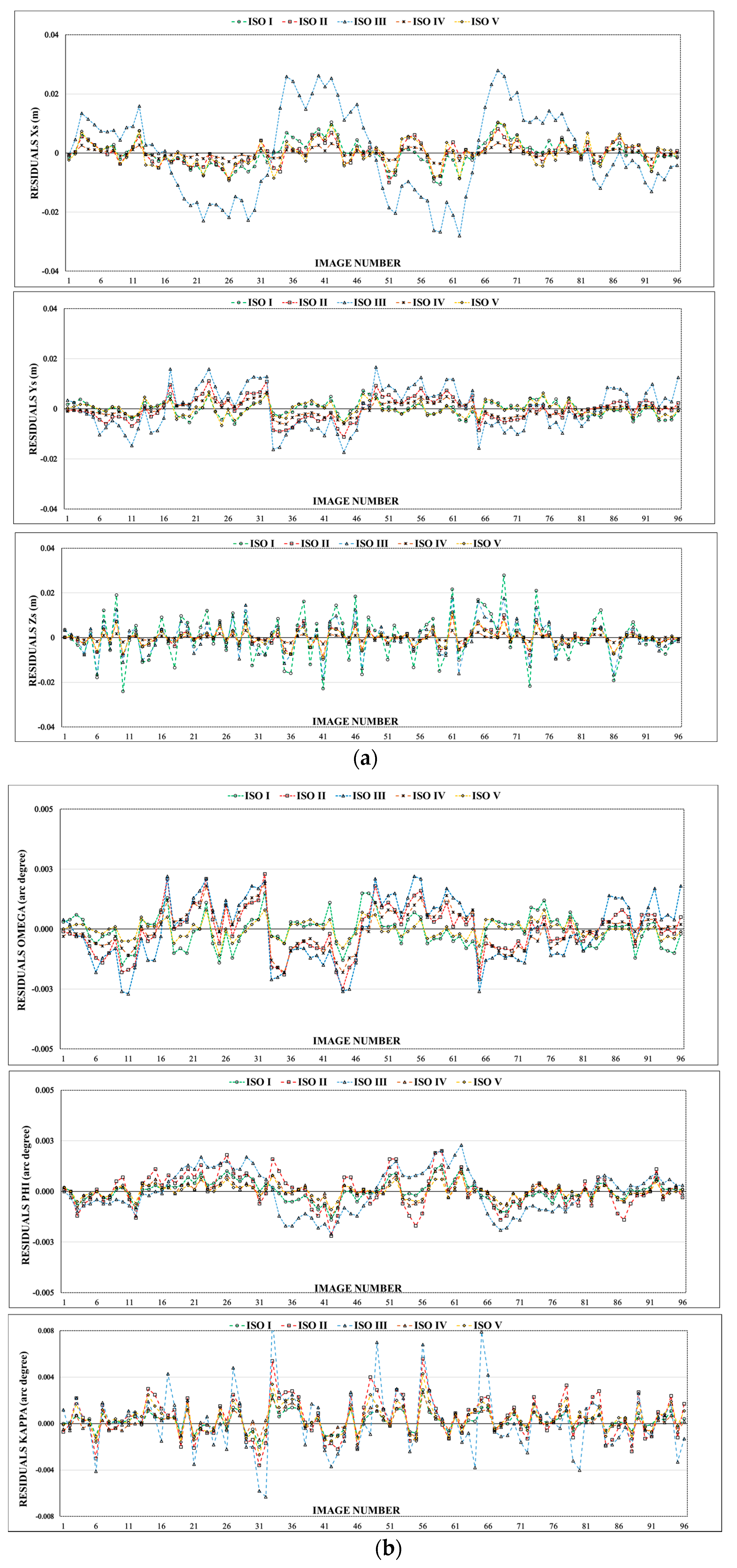
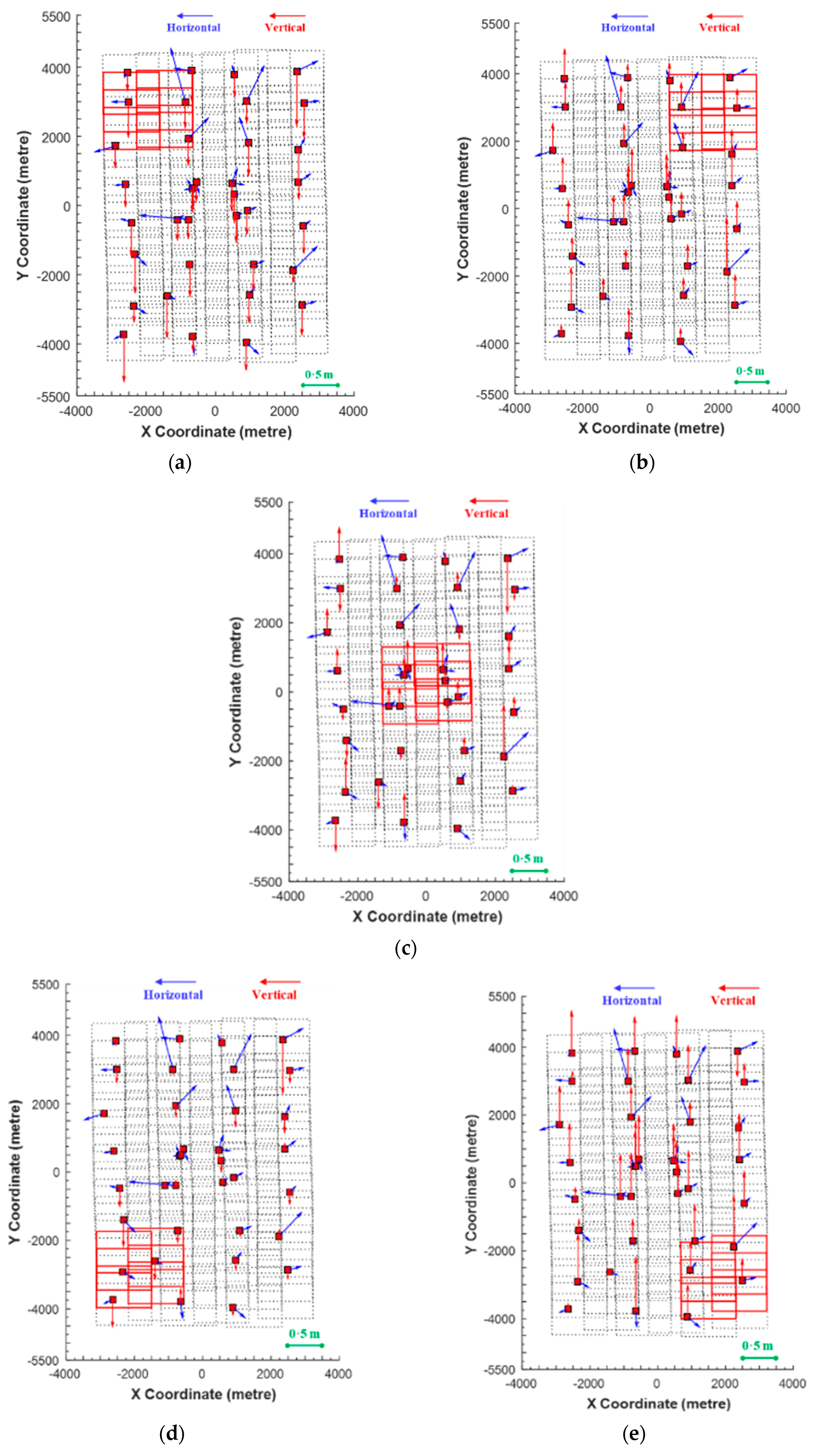
Figure 2 shows graphically the residuals of the direct measurement of the camera exposure stations from the five ISO sub-block experiments. Figure 2a shows the position residuals of the camera stations (X_s, Y_s, Z_s); despite the fact that all the ISO experiments have residuals values according to a priori adopted precisions, the ISO sub-block III has greater residuals in (X_s, Y_s) components than others ISO experiments and the ISO sub-block I has the largest value residuals in the Z_s component.

Figure 2b shows the orientation residuals of the camera stations (ω, φ, κ). All orientation residuals from the five ISO experiments have values according to a priori adopted values. However, the largest values of orientation residuals in ω, φ and κ components were connected to ISO sub-block II and III experiments.

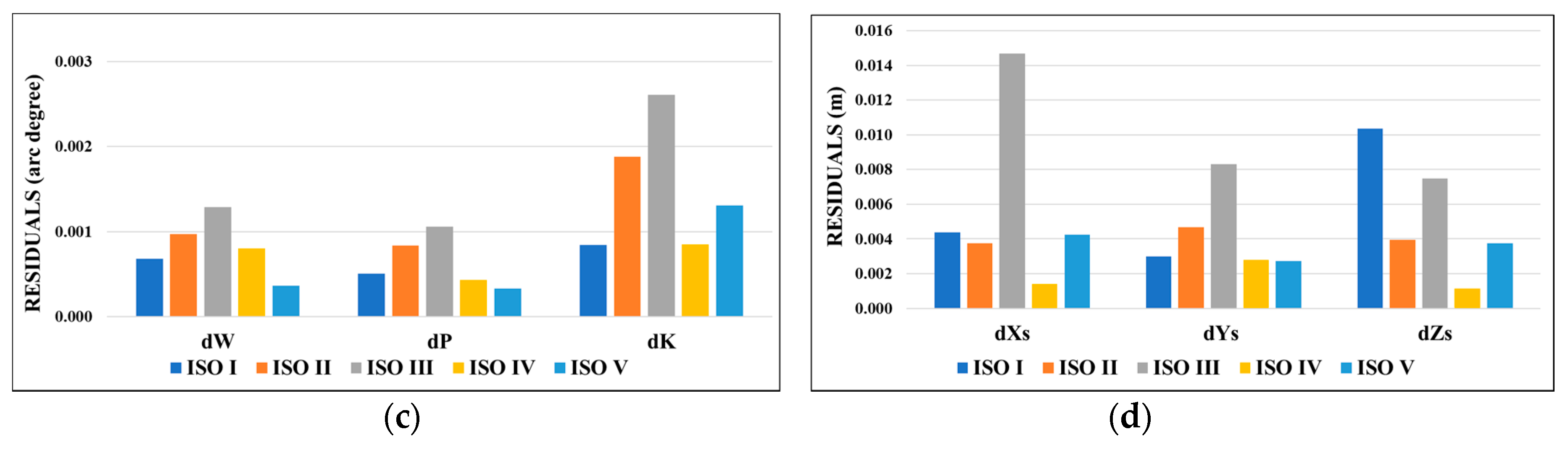
Considering the values of the RMSE of the measurement residuals obtained from the five ISO sub-block experiments (shown in Table 3 and Figure 2c,d), it can be concluded that the ISO sub-block II and III experiments have lower measurement precisions than the other ISO experiments. On the other hand, the ISO experiment sub-block IV has higher measurement precisions than others.

Table 4 shows the main results of the 3D LCP check point discrepancies, performed after the ISO experiments using different sets of IOP. A closer look at the horizontal (DH RMSE) from the five ISO sub-block experiments reveals that the obtained planimetric accuracies were nearly the same; despite significant differences in focal distances, found in sub-block II and III, the values of DH RMSE ranged from of 47.5 cm to 48.6 cm. However as expected, the vertical accuracy did not have the same behavior. Among the five ISO sub-block experiments, the values of DZ RMSE ranged from 23.5 cm to 72.6 cm. The lower value of vertical accuracy (DZ RMSE) was achieved in the ISO experiment using IOP from sub-block I; the vertical RMSE value (23.5 cm) was nearly half of the vertical ISO precision accepted for this study (41 cm). In addition, the mean of vertical discrepancies is nearly zero, showing an ISO experiment with insignificant systematic errors.

Figure 3 shows the vector graphs of the horizontal and vertical discrepancies computed from the five ISO sub-block experiments. It can be seen that the horizontal discrepancies do not have a significant systematic error. In general, the horizontal vectors have diffuse directions in the five ISO sub-block experiments. However, the LCPs (check points) positioned at the first right strip have their horizontal vectors pointed in the same direction. In addition, the LCPs (check points), positioned at the north region of the image block have larger horizontal discrepancies than other check points. These two characteristics can indicate some small systematic error not modelled in these regions of the image block.

In contrast to the horizontal discrepancies, the vertical discrepancies from the ISO sub-block II, III and V experiments have significant tendencies as can be seen in Figure 3a,b,e. In these vector graphs all vertical vectors are pointed to north or south directions indicating a small systematic error not modelled in these ISO sub-block experiments. On the other hand, the vertical discrepancies from the ISO sub-block I and IV experiments have insignificant tendencies as can be seen in Figure 3c,d.

As expected, the better vertical accuracy from the ISO experiments performed was achieved when IOP were estimated simultaneously using the entire image block with four LCPs positioned at the block’s corners. The value of vertical RMSE obtained in this experiment was equal to 21.4 cm and the mean value of the vertical discrepancies was also close to zero. Based on the results obtained from these experiments, the ISO sub-block I and IV achieved the best results. However, the vertical RMSE of ISO sub-block I was slightly smaller than ISO sub-block IV (about 5 cm), which indicates that a small sub-block positioned at the center of the entire image block can be recommended.

4. Conclusions

This paper presented a study of the influence of the sub-block position in the entire image block on the performance of integrated sensor orientation using in situ camera calibration and Lidar control points. Five sub-blocks were extracted from the entire image block to estimate IOP under in-flight conditions by in situ calibrations. Five ISO experiments, using the entire image block, were performed as the reference set. Another ISO experiment with in situ calibration was performed as the reference. The main conclusions are as follows:

(a)

In all sub-block in situ calibrations, the values of the principal point coordinates are nearly the same. This implies that the position of the sub-block at the entire image block is not significant for performing this estimation.

(b)

Considering only horizontal accuracy, the sub-block position at the entire image block was not important to estimating IOP under in-flight conditions in order to perform ISO experiments due to the horizontal RMSE of check point discrepancies, which were nearly the same for all ISO experiments.

(c)

As expected, the ISO experiment with simultaneous in situ calibration, using the entire block with four Lidar control points (LCPs) positioned at the corners, achieved the lowest horizontal and vertical RMSE from the check point discrepancies, confirming its application as the reference value in this study.

(d)

By contrast, with the principal point coordinates the focal length varied significantly in the three sub-blocks in situ calibrations; the maximum variation was 50 µm between sub-blocks II and III. This variation may be related to the inaccuracies of the LCPs or the camera station coordinates.

(e)

The ISO sub-block I and IV calibrations achieved nearly the same focal length; the vertical accuracies obtained from the ISO sub-blocks I and II were close to the vertical reference accuracy. Nevertheless, the RMSE of the vertical discrepancies in ISO sub-block I was slightly smaller than ISO sub-block IV. It can be empirically concluded that a small sub-block of images, positioned at the center of the entire image block, can be recommended.

(f)

The ISO experiments performed in this study highlight the importance of IOP, estimated in flight conditions, to improve the horizontal and vertical accuracies of Lidar and photogrammetric dataset integration. Although four LCPs were used to perform the ISO with the manufacturer’s IOP, the RMSE of the horizontal and vertical check point discrepancies did not achieve acceptable results.

(g)

The estimation of IOP in flight conditions using sub-block calibration inside the entire image block increased the accuracies in the ISO experiment without LCPs. Despite the fact that in situ calibration requires LCPs, the quantity of LCPS is small (two horizontal and vertical and only one vertical) inside a small image sub-block.

Future work will focus on the boresight refinement and IOP estimation in flight conditions through sub-block and LCPs approaches in order to increase the direct sensor orientation (DSO) for Lidar and photogrammetric dataset integration.