TS2uRF: A New Method for Sharpening Thermal Infrared Satellite Imagery

 ,
,  ,
, 

Abstract
:
1. Introduction
2. Materials and Methods
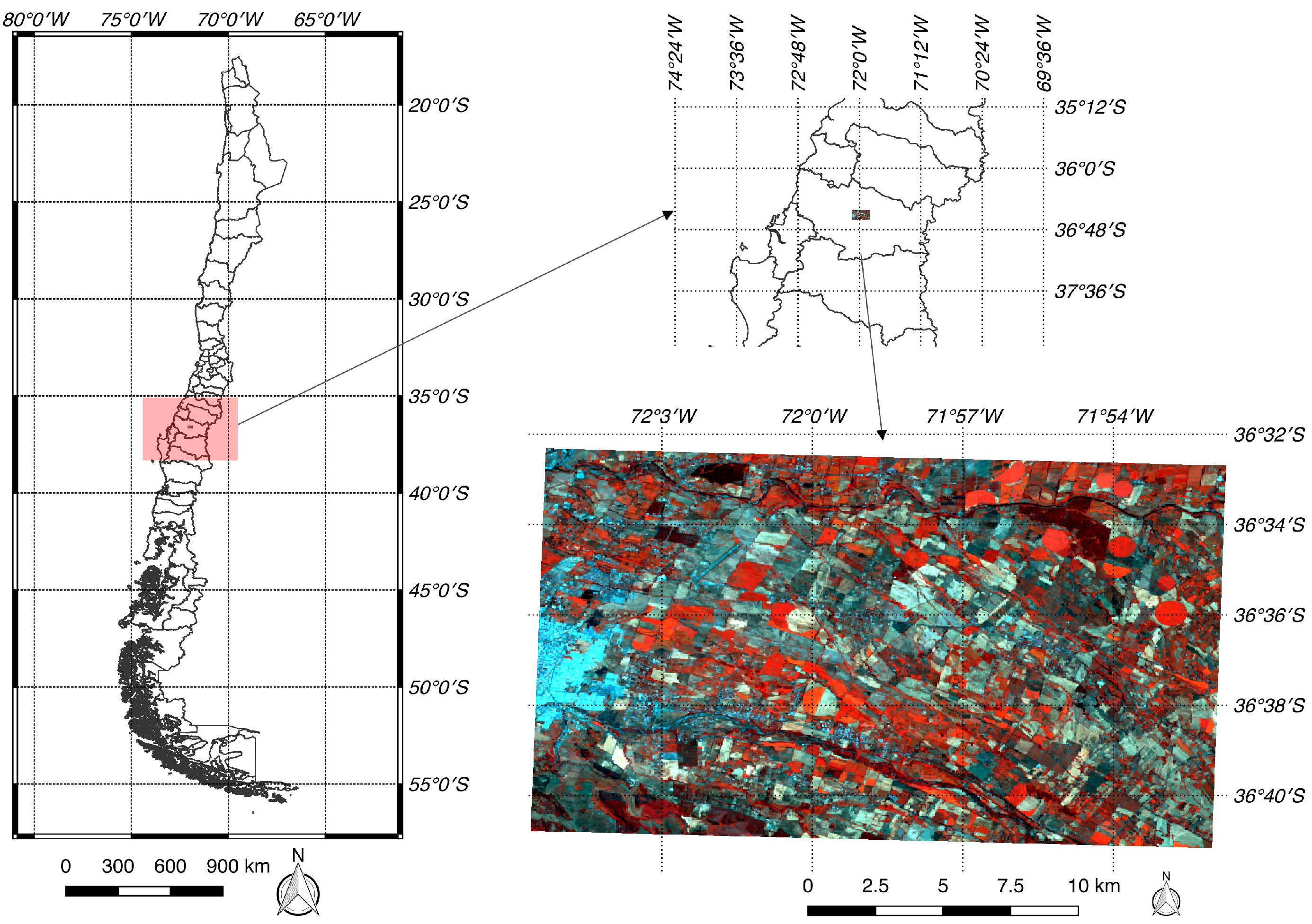
2.1. Study Site
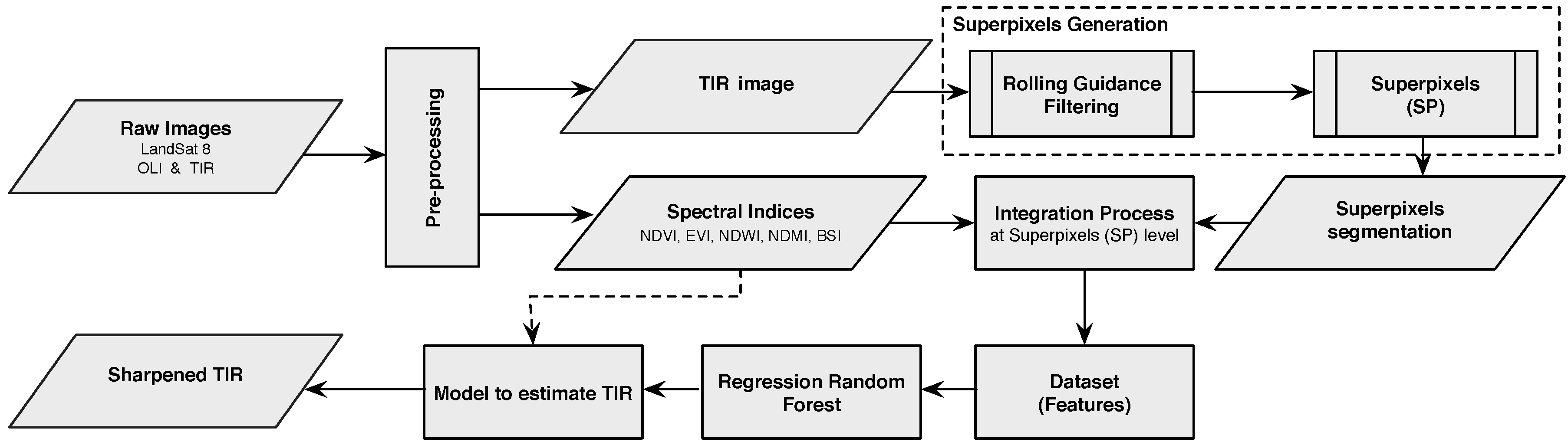
2.2. Methodology
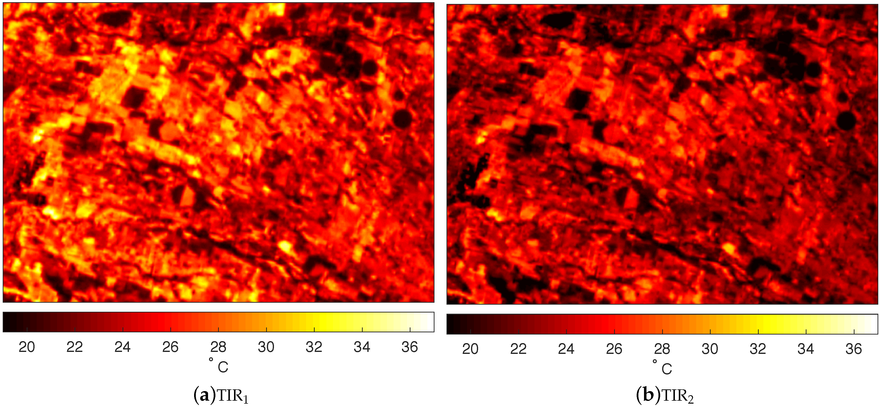
2.2.1. Preprocessing
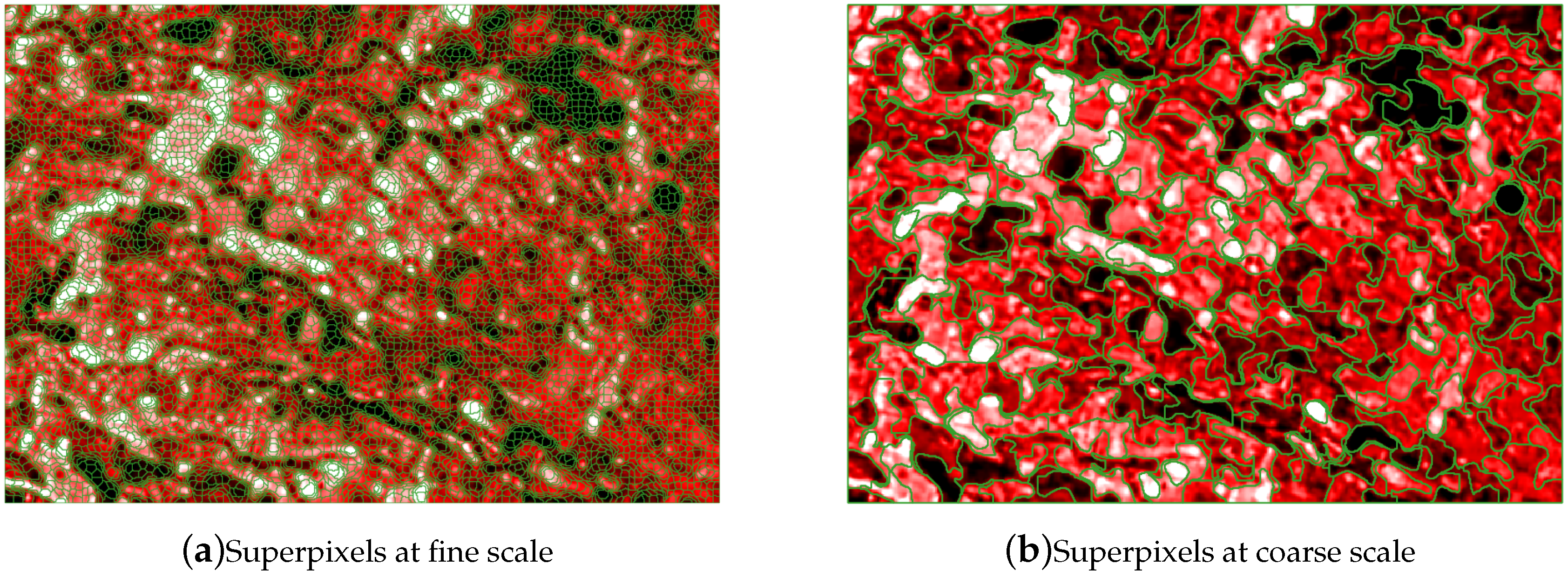
2.2.2. Superpixel Generation
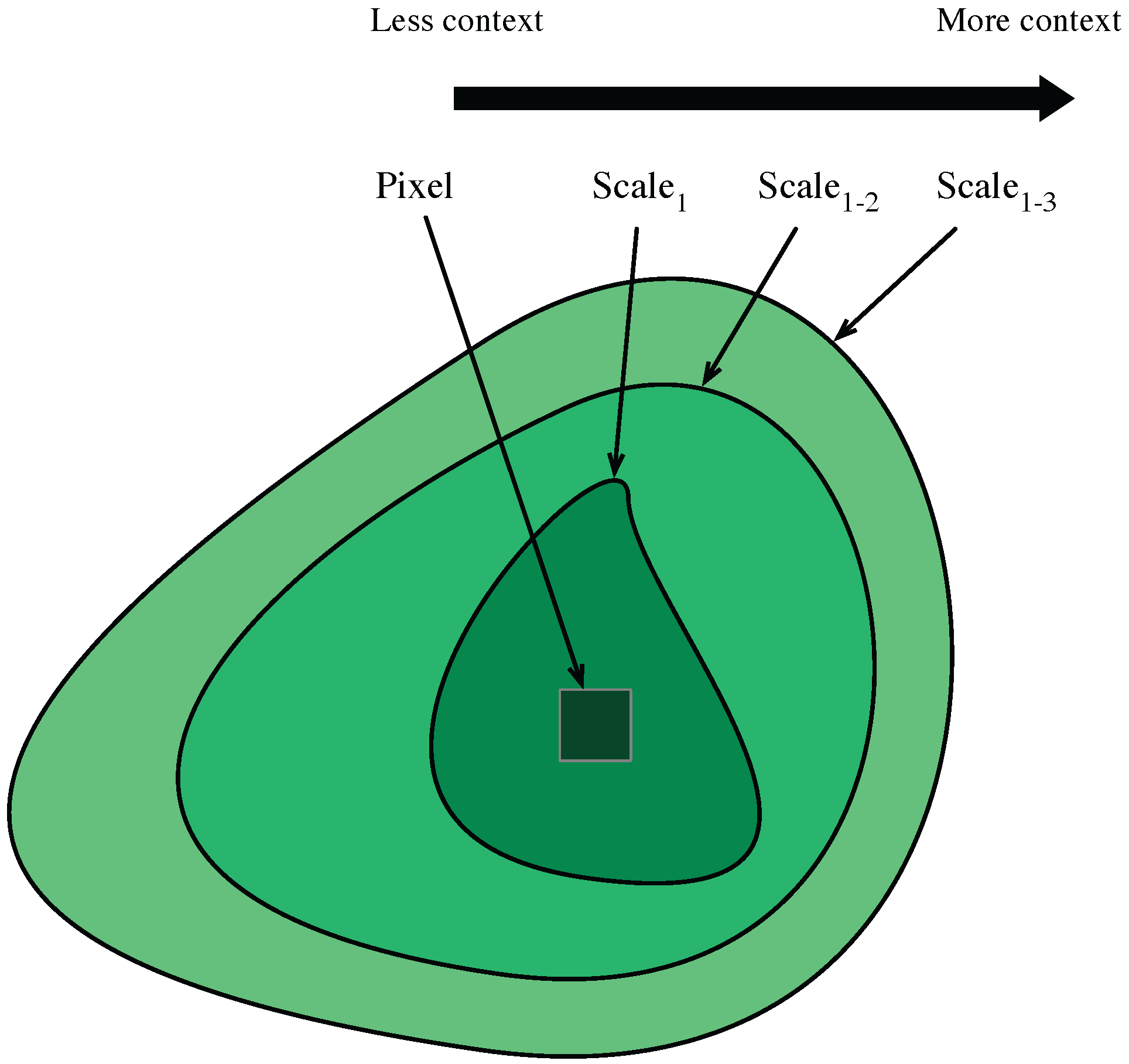
2.2.3. Integration Process
2.2.4. Regression Random Forest Model Generation
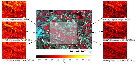
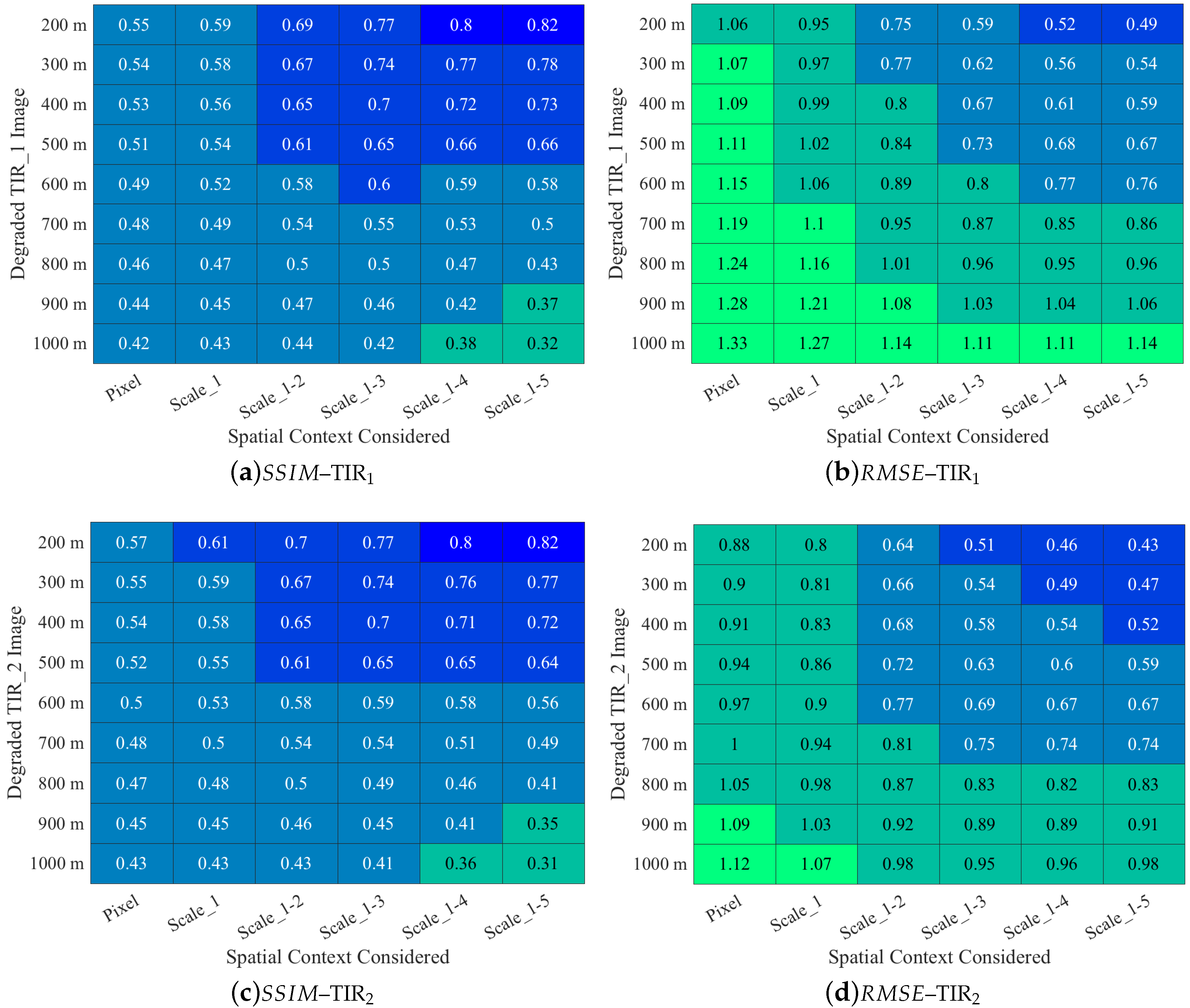
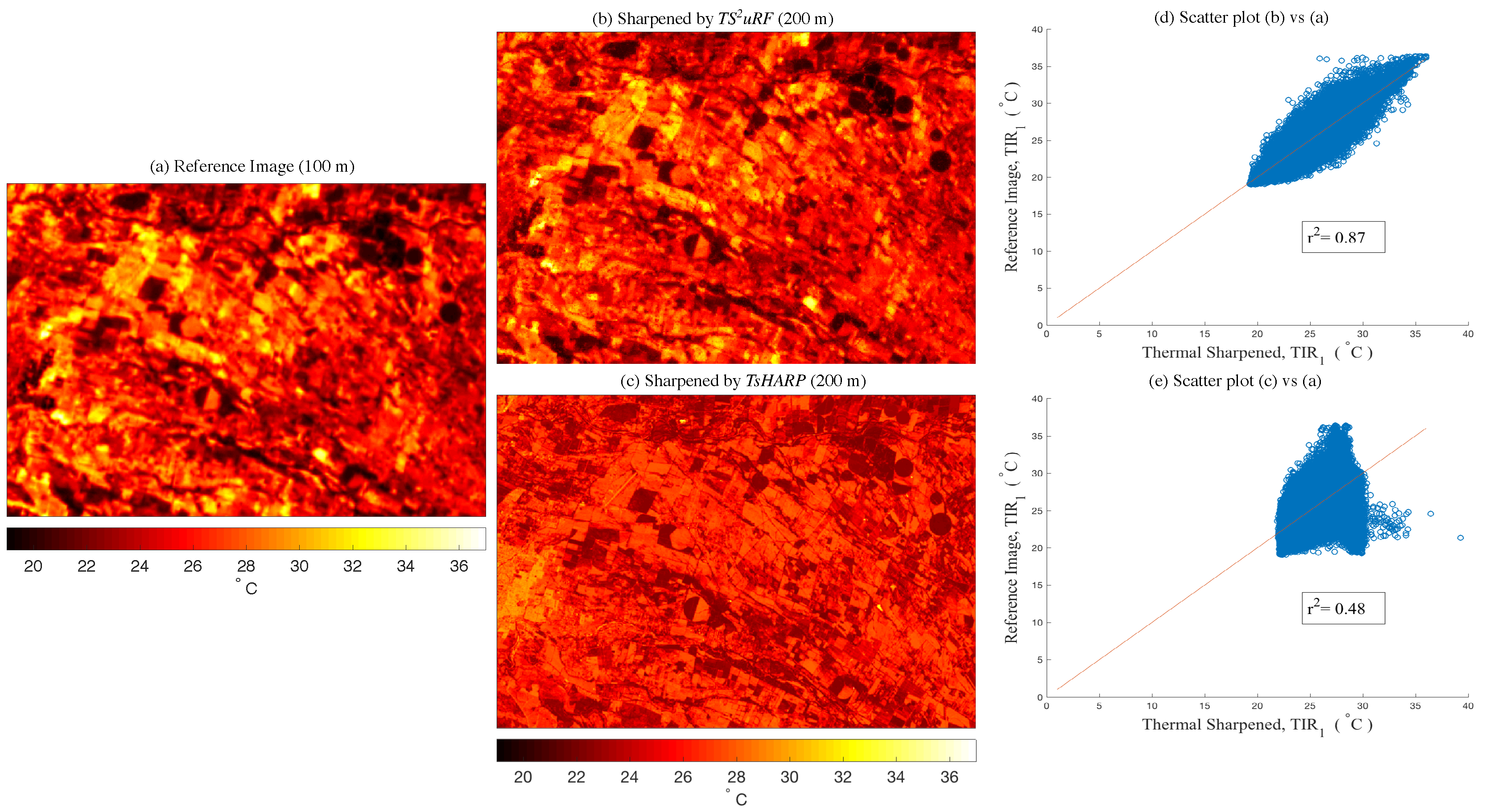
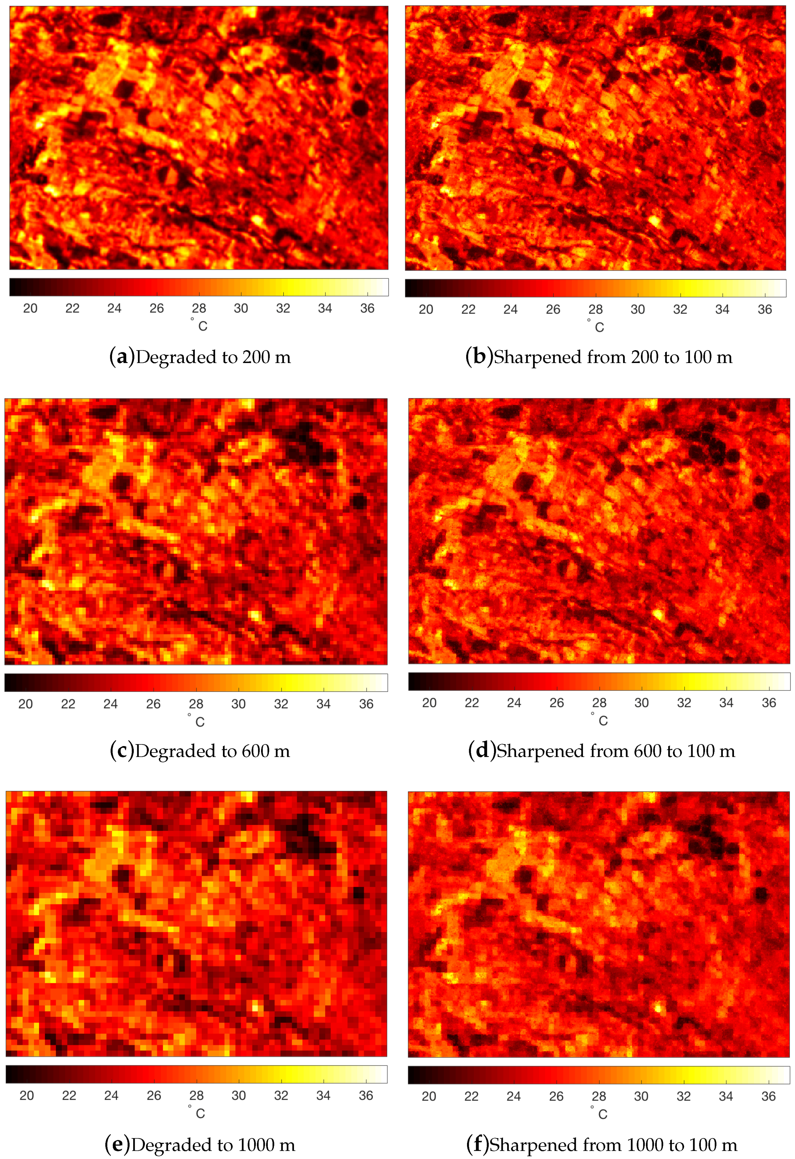
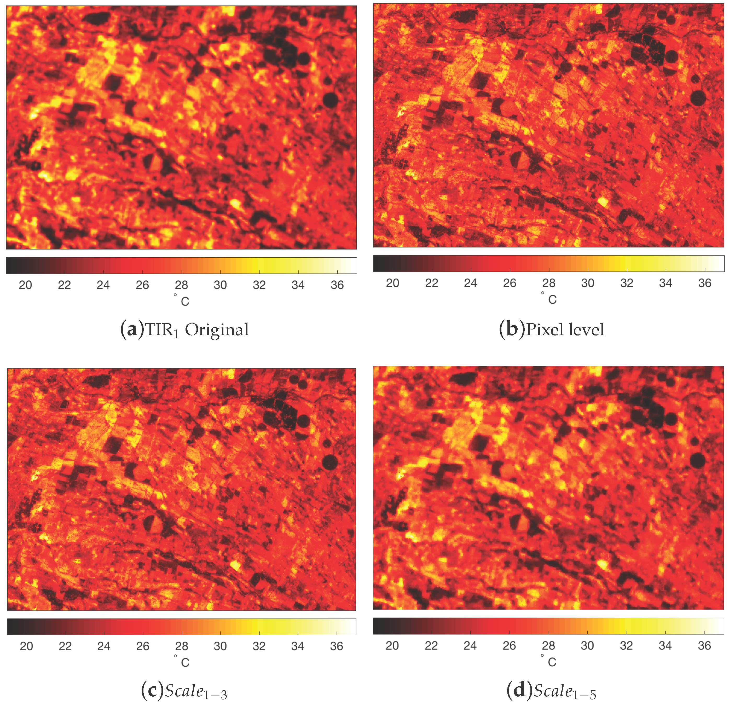
3. Results
4. Discussion
5. Conclusions
Acknowledgments
Author Contributions
Conflicts of Interest
References
- Seelan, S.K.; Laguette, S.; Casady, G.M.; Seielstad, G.A. Remote sensing applications for precision agriculture: A learning community approach. Remote Sens. Environ. 2003, 88, 157–169. [Google Scholar] [CrossRef]
- Meneti, M.; Choudhary, B. Parameterization of land surface evapotranspiration using a location dependent potential evapotranspiration and surface temperature range. In Exchange Processes at the Land Surface for a Range of Space and Time Scales; Bolle, H.J., Feddes, R.A., Kalma, J.D., Eds.; International Association of Hydrological Sciences Publication: London, UK, 1993; Volume 212, pp. 561–568. [Google Scholar]
- Kustas, W.; Norman, J. Evaluation of soil and vegetation heat flux predictions using a simple two-source model with radiometric temperatures for partial canopy cover. Agric. For. Meteorol. 1999, 94, 13–29. [Google Scholar] [CrossRef]
- Allen, R.; Tasumi, M.; Trezza, R. Satellite-based energy balance for mapping evapotranspiration with internalized calibration (METRIC)—Model. J. Irrig. Drain. Eng. 2007, 133, 380–394. [Google Scholar] [CrossRef]
- Bastiaanssen, W.; Meneti, M.; Feddes, R.; Holtslag, A. A remote sensing surface energy balance algorithm for land (SEBAL). Formulation. J. Hydrol. 1998, 212–213, 198–212. [Google Scholar] [CrossRef]
- Ishimwe, R.; Abutaleb, K.; Ahmed, F. Applications of thermal imaging in agriculture—A review. Adv. Remote Sens. 2014, 3, 128. [Google Scholar] [CrossRef]
- Cammalleri, C.; Ciraolo, G.; Minacapilli, M. Spatial sharpening of land surface temperature for daily energy balance applications. In Remote Sensing for Agriculture, Ecosystems, and Hydrology X; International Society for Optics and Photonics: Bellingham, WA, USA, 2008; Volume 7104, p. 71040J. [Google Scholar]
- Zhan, W.; Chen, Y.; Zhou, J.; Li, J.; Liu, W. Sharpening Thermal Imageries: A Generalized Theoretical Framework From an Assimilation Perspective. IEEE Trans. Geosci. Remote Sens. 2011, 49, 773–789. [Google Scholar] [CrossRef]
- Chen, Y.; Zhan, W.; Quan, J.; Zhou, J.; Zhu, X.; Sun, H. Disaggregation of Remotely Sensed Land Surface Temperature: A Generalized Paradigm. IEEE Trans. Geosci. Remote Sens. 2014, 52, 5952–5965. [Google Scholar] [CrossRef]
- Zhan, W.; Chen, Y.; Zhou, J.; Wang, J.; Liu, W.; Voogt, J.; Zhu, X.; Quan, J.; Li, J. Disaggregation of remotely sensed land surface temperature: Literature survey, taxonomy, issues, and caveats. Remote Sens. Environ. 2013, 131, 119–139. [Google Scholar] [CrossRef]
- Bai, Y.; Wong, M.S.; Shi, W.Z.; Wu, L.X.; Qin, K. Advancing of Land Surface Temperature Retrieval Using Extreme Learning Machine and Spatio-Temporal Adaptive Data Fusion Algorithm. Remote Sens. 2015, 7, 4424–4441. [Google Scholar] [CrossRef]
- Kustas, W.P.; Norman, J.M.; Anderson, M.C.; French, A.N. Estimating subpixel surface temperatures and energy fluxes from the vegetation index–radiometric temperature relationship. Remote Sens. Environ. 2003, 85, 429–440. [Google Scholar] [CrossRef]
- Agam, N.; Kustas, W.P.; Anderson, M.C.; Li, F.; Neale, C.M. A vegetation index based technique for spatial sharpening of thermal imagery. Remote Sens. Environ. 2007, 107, 545–558. [Google Scholar] [CrossRef]
- Agam, N.; Kustas, W.P.; Anderson, M.C.; Li, F.; Colaizzi, P.D. Utility of thermal sharpening over Texas high plains irrigated agricultural fields. J. Geophys. Res. Atmos. 2007, 112, D19110. [Google Scholar] [CrossRef]
- Chen, X.; Li, W.; Chen, J.; Rao, Y.; Yamaguchi, Y. A Combination of TsHARP and Thin Plate Spline Interpolation for Spatial Sharpening of Thermal Imagery. Remote Sens. 2014, 6, 2845–2863. [Google Scholar] [CrossRef]
- Dominguez, A.; Kleissl, J.; Luvall, J.C.; Rickman, D.L. High-resolution urban thermal sharpener (HUTS). Remote Sens. Environ. 2011, 115, 1772–1780. [Google Scholar] [CrossRef]
- Jeganathan, C.; Hamm, N.; Mukherjee, S.; Atkinson, P.M.; Raju, P.; Dadhwal, V. Evaluating a thermal image sharpening model over a mixed agricultural landscape in India. Int. J. Appl. Earth Obs. Geoinf. 2011, 13, 178–191. [Google Scholar] [CrossRef]
- Gao, F.; Kustas, W.P.; Anderson, M.C. A Data Mining Approach for Sharpening Thermal Satellite Imagery over Land. Remote Sens. 2012, 4, 3287–3319. [Google Scholar] [CrossRef]
- Huang, G.B.; Zhu, Q.Y.; Siew, C.K. Extreme learning machine: Theory and applications. Neurocomputing 2006, 70, 489–501. [Google Scholar] [CrossRef]
- Schöpfer, E.; Lang, S.; Strobl, J. Segmentation and object-based image analysis. In Remote Sensing of Urban and Suburban Areas; Springer: Berlin, Germany, 2010; pp. 181–192. [Google Scholar]
- Zhan, W.; Chen, Y.; Wang, J.; Zhou, J.; Quan, J.; Liu, W.; Li, J. Downscaling land surface temperatures with multi-spectral and multi-resolution images. Int. J. Appl. Earth Obs. Geoinf. 2012, 18, 23–36. [Google Scholar] [CrossRef]
- Garcia-Pedrero, A.; Gonzalo-Martin, C.; Fonseca-Luengo, D.; Lillo-Saavedra, M. A GEOBIA methodology for fragmented agricultural landscapes. Remote Sens. 2015, 7, 767–787. [Google Scholar] [CrossRef]
- Ortiz Toro, C.A.; Gonzalo Martin, C.; Garcia Pedrero, A.; Menasalvas Ruiz, E. Superpixel-Based Roughness Measure for Multispectral Satellite Image Segmentation. Remote Sens. 2015, 7, 14620–14645. [Google Scholar] [CrossRef]
- Blaschke, T.; Kelly, M.; Merschdorf, H. Object-Based Image Analysis: Evolution, History, State of the Art, and Future Vision. In Remotely Sensed Data Characterization, Classification, and Accuracies; CRC Press: Boca Raton, FL, USA, 2015; pp. 277–294. [Google Scholar]
- Huang, X.; Yang, W.; Xia, G.S.; Liao, M. Superpixel-based change detection in high resolution sar images using region covariance features. In Proceedings of the 8th International Workshop on the Analysis of Multitemporal Remote Sensing Images, Annecy, France, 22–24 July 2015; pp. 1–4. [Google Scholar]
- Priya, T.; Prasad, S.; Wu, H. Superpixels for spatially reinforced bayesian classification of hyperspectral images. IEEE Geosci. Remote Sens. Lett. 2015, 12, 1071–1075. [Google Scholar] [CrossRef]
- Vargas, J.; Falcao, A.; dos Santos, J.; Esquerdo, J.; Coutinho, A.; Antunes, J. Contextual superpixel description for remote sensing image classification. In Proceedings of the IEEE International Geoscience and Remote Sensing Symposium, Milan, Italy, 26–31 July 2015; pp. 1132–1135. [Google Scholar]
- Moran, M.S.; Jackson, R.D.; Slater, P.N.; Teillet, P.M. Evaluation of simplified procedures for retrieval of land surface reflectance factors from satellite sensor output. Remote Sens. Environ. 1992, 41, 169–184. [Google Scholar] [CrossRef]
- Congedo, L. Semi-automatic classification plugin documentation. Release 2016, 4, 29. [Google Scholar]
- QGIS Development Team. QGIS Geographic Information System; Open Source Geospatial Foundation Project. Available online: http://qgis.osgeo.org (accessed on 6 February 2018).
- Ren, X.; Malik, J. Learning a classification model for segmentation. In Proceedings of the Ninth IEEE International Conference on Computer Vision, Nice, France, 13–16 October 2003; Volume 1, pp. 10–17. [Google Scholar]
- Achanta, R.; Shaji, A.; Smith, K.; Lucchi, A.; Fua, P.; Süsstrunk, S. Slic Superpixels; Techque Report; École Polytechnique Fédéral de Lausssanne (EPFL): Lausanne, Switzerland, 2010; p. 149300. [Google Scholar]
- Gonzalo-Martín, C.; Lillo-Saavedra, M.; Menasalvas, E.; Fonseca-Luengo, D.; García-Pedrero, A.; Costumero, R. Local optimal scale in a hierarchical segmentation method for satellite images. J. Intell. Inf. Syst. 2016, 46, 517–529. [Google Scholar] [CrossRef]
- Zhang, Q.; Shen, X.; Xu, L.; Jia, J. Rolling guidance filter. In European Conference on Computer Vision; Springer: Cham, Switzerland, 2014; pp. 815–830. [Google Scholar]
- Li, P.; Jiang, L.; Feng, Z. Cross-comparison of vegetation indices derived from Landsat-7 enhanced thematic mapper plus (ETM+) and Landsat-8 operational land imager (OLI) sensors. Remote Sens. 2013, 6, 310–329. [Google Scholar] [CrossRef]
- Breiman, L.; Friedman, J.; Stone, C.J.; Olshen, R.A. Classification and Regression Trees; CRC Press: Boca Raton, DL, USA, 1984. [Google Scholar]
- Breiman, L. Random Forests. Mach. Learn. 2001, 45, 5–32. [Google Scholar] [CrossRef]


| # Band | Name Band | Bandwidth (μm) | Spatial Res. (m) |
|---|---|---|---|
| Band 1 | Coastal/Aerosol | 0.435–0.451 | 30 |
| Band 2 | Blue | 0.452–0.512 | 30 |
| Band 3 | Green | 0.533–0.590 | 30 |
| Band 4 | Red | 0.636–0.673 | 30 |
| Band 5 | NIR | 0.851–0.879 | 30 |
| Band 6 | SWIR | 1.566–1.651 | 30 |
| Band 7 | SWIR | 2.107–2.294 | 30 |
| Band 8 | PAN | 0.503–0.676 | 15 |
| Band 9 | Cirrus | 1.363–1.384 | 30 |
| Band10 | TIR | 10.60–11.90 | 100 |
| Band11 | TIR | 11.50–12.51 | 100 |
| Index | Equation Using Landsat 8 OLI [35] |
|---|---|
| Normalized Difference Vegetation Index (NDVI) | |
| Enhanced Vegetation Index (EVI) | |
| Normalized Difference Water Index (NDWI) | |
| Normalized Difference Moisture Index (NDMI) | |
| Bare Soil Index (BSI) |
| TIR | TSuRF ( TIR at 100 m) | TsHARP (TIR at 100 m) | ||||
|---|---|---|---|---|---|---|
| Degraded | Spatial Context | SSIM | RMSE (°C) | Spatial Context | SSIM | RMSE (°C) |
| 200 m | 0.824 | 0.490 | Pixel Level | 0.412 | 1.906 | |
| 300 m | 0.784 | 0.540 | 0.414 | 1.907 | ||
| 400 m | 0.730 | 0.592 | 0.415 | 1.910 | ||
| 500 m | 0.660 | 0.670 | 0.417 | 1.915 | ||
| 600 m | 0.654 | 0.765 | 0.419 | 1.924 | ||
| 700 m | 0.601 | 0.871 | 0.419 | 1.933 | ||
| 800 m | 0.550 | 0.960 | 0.420 | 1.945 | ||
| 900 m | 0.500 | 1.034 | 0.419 | 1.960 | ||
| 1000 m | 0.421 | 1.110 | 0.419 | 1.972 | ||
© 2018 by the authors. Licensee MDPI, Basel, Switzerland. This article is an open access article distributed under the terms and conditions of the Creative Commons Attribution (CC BY) license (http://creativecommons.org/licenses/by/4.0/).
Share and Cite
Lillo-Saavedra, M.; García-Pedrero, A.; Merino, G.; Gonzalo-Martín, C. TS2uRF: A New Method for Sharpening Thermal Infrared Satellite Imagery. Remote Sens. 2018, 10, 249. https://doi.org/10.3390/rs10020249
Lillo-Saavedra M, García-Pedrero A, Merino G, Gonzalo-Martín C. TS2uRF: A New Method for Sharpening Thermal Infrared Satellite Imagery. Remote Sensing. 2018; 10(2):249. https://doi.org/10.3390/rs10020249
Chicago/Turabian StyleLillo-Saavedra, Mario, Angel García-Pedrero, Gabriel Merino, and Consuelo Gonzalo-Martín. 2018. "TS2uRF: A New Method for Sharpening Thermal Infrared Satellite Imagery" Remote Sensing 10, no. 2: 249. https://doi.org/10.3390/rs10020249
APA StyleLillo-Saavedra, M., García-Pedrero, A., Merino, G., & Gonzalo-Martín, C. (2018). TS2uRF: A New Method for Sharpening Thermal Infrared Satellite Imagery. Remote Sensing, 10(2), 249. https://doi.org/10.3390/rs10020249