Hue-Angle Product for Low to Medium Spatial Resolution Optical Satellite Sensors


Abstract

1. Introduction
2. Materials and Methods
2.1. Satellite Colourimetry
2.2. Synthetic and Field Spectra
2.3. Satellite Simulated Spectra
3. Results
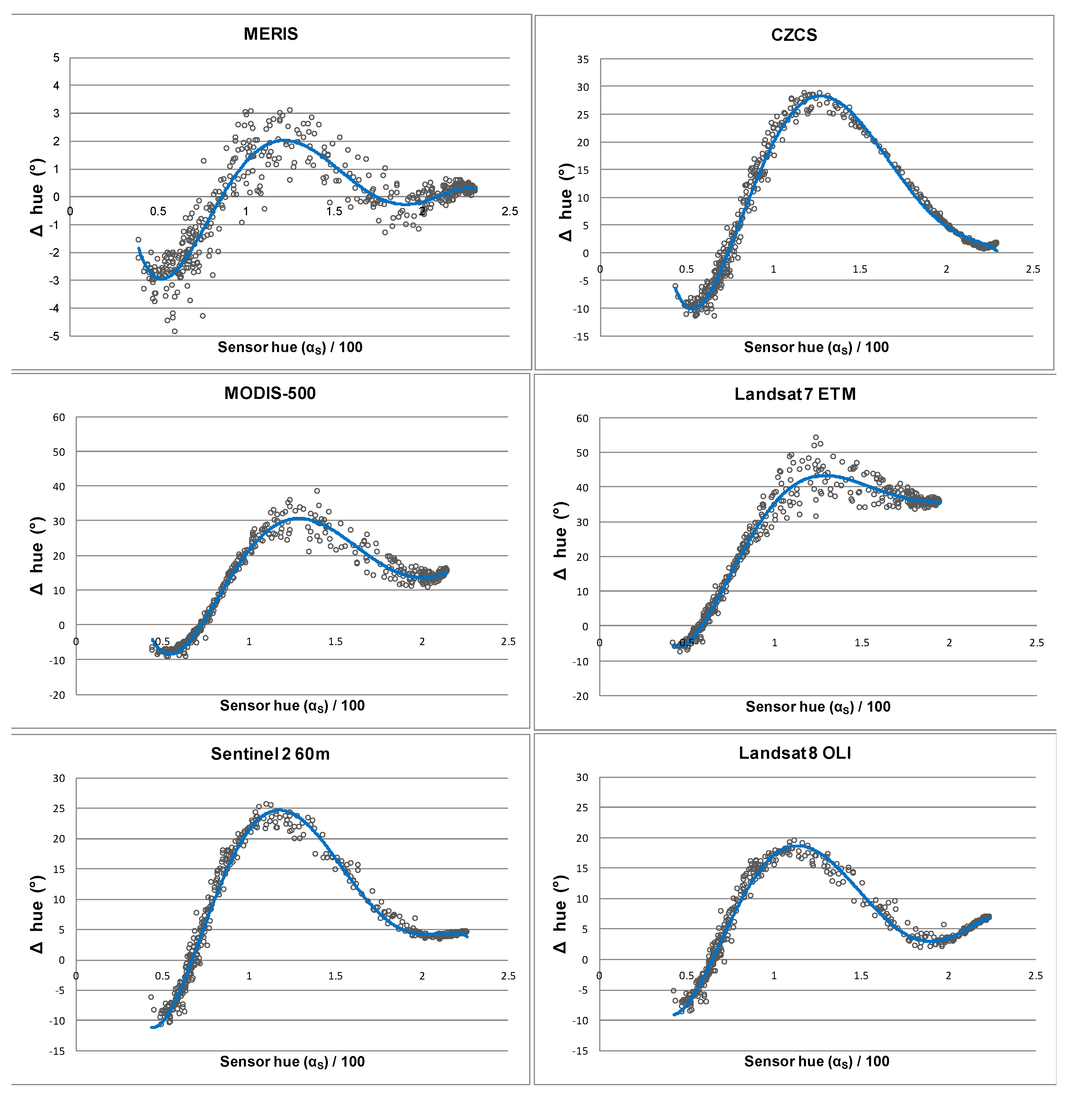
3.1. Sensor Algorithms
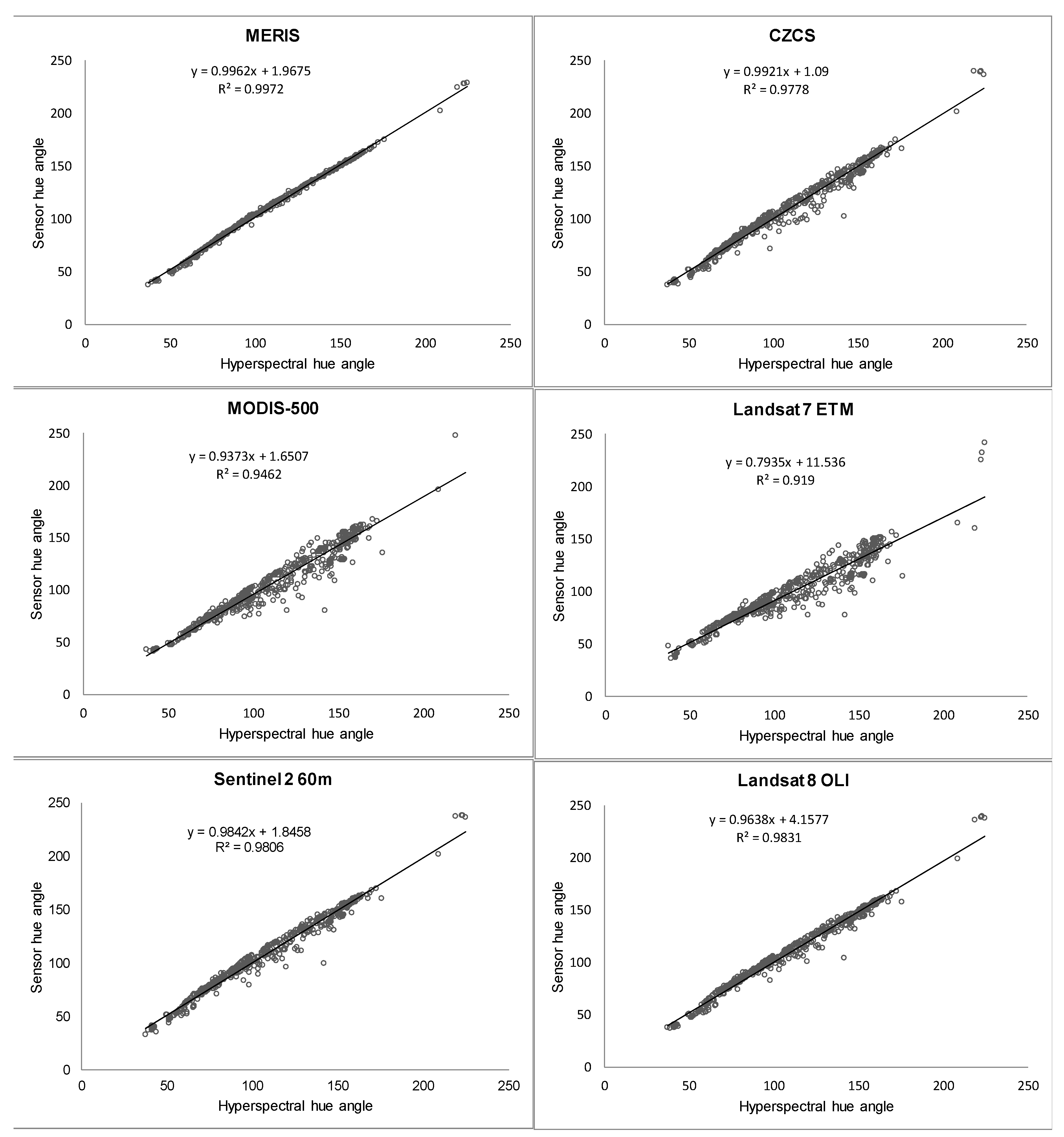
3.2. Algorithm Validation
3.3. Accuracy
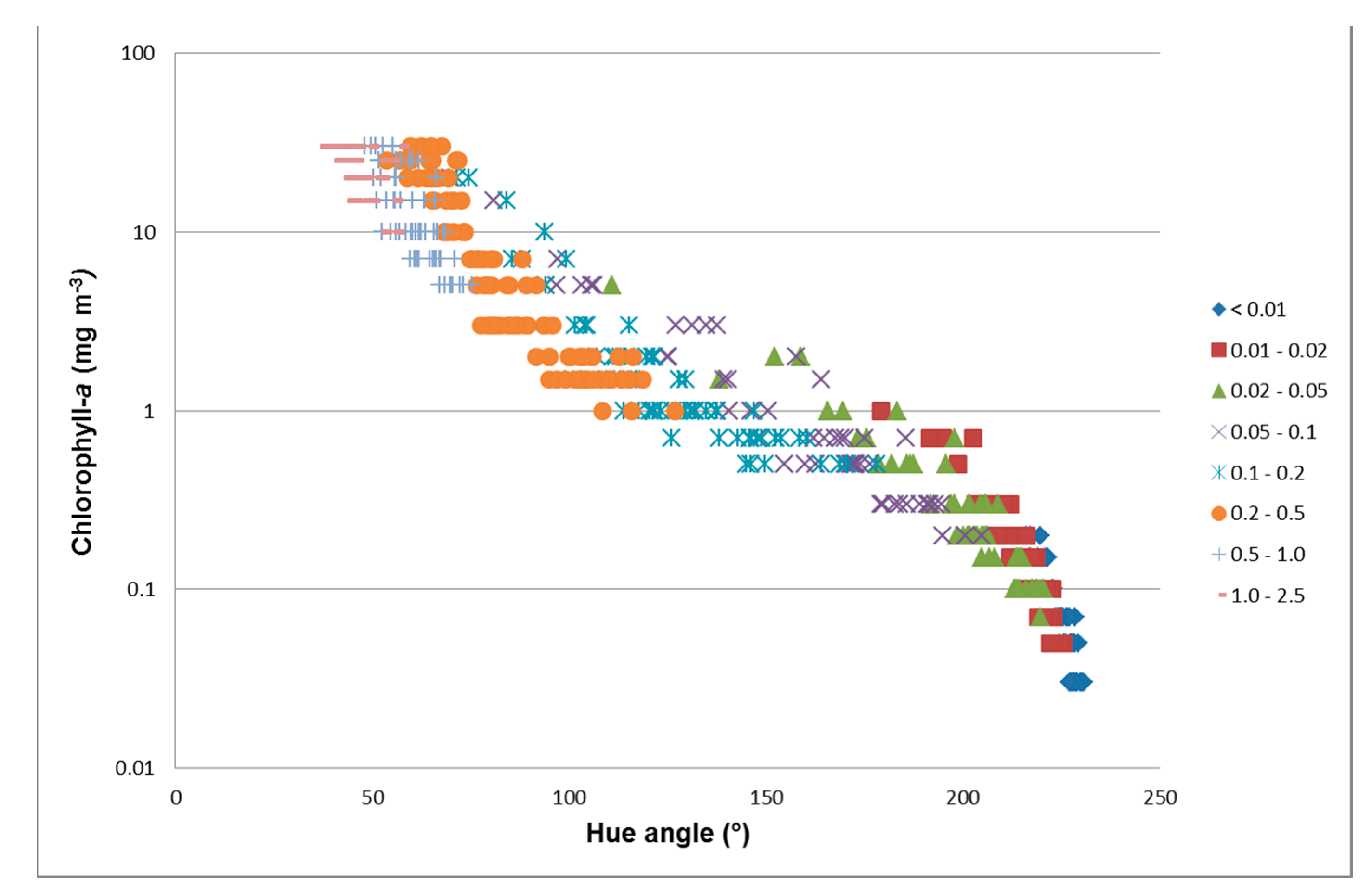
3.4. The Use of Hue
4. Discussion
5. Conclusions
Acknowledgments
Author Contributions
Conflicts of Interest
References
- Van der Woerd, H.J.; Wernand, M.R. True colour classification of natural waters with medium-spectral resolution satellites: SeaWiFS, MODIS, MERIS and OLCI. Sensors 2015, 15, 25663–25680. [Google Scholar] [CrossRef] [PubMed]
- Commission Internationale de l’Éclairage Proceedings, 1931; Cambridge University Press: Cambridge, UK, 1932.
- Wyszecki, G.; Stiles, W.S. Color Science: Concepts and Methods, Quantitative Data and Formulae; John Wiley & Sons: New York, NY, USA, 1982. [Google Scholar]
- Citclops (Citizens’ Observatory for Coast and Ocean Optical Monitoring). Available online: www.citclops.eu (accessed on 29 July 2017).
- Busch, J.A.; Badají, R.; Ceccaroni, L.; Friedrichs, A.; Piera, J.; Simon, C.; Thijsse, P.; Wernand, M.; Van der Woerd, H.J.; Zielinski, O. Citizen bio-optical observations from coast- and ocean and their compatibility with ocean colour satellite measurements. Remote Sens. 2016, 8, 879. [Google Scholar] [CrossRef]
- Dickinson, J.L.; Shirk, J.; Bonter, D.; Bonney, R.; Crain, R.L.; Martin, J.; Phillips, T.; Purcell, K. The current state of citizen science as a tool for ecological research and public engagement. Front. Ecol. Environ. 2012, 10, 291–297. [Google Scholar] [CrossRef]
- Tulloch, A.I.T.; Possingham, H.P.; Joseph, L.N.; Szabo, J.; Martin, T.G. Realising the full potential of citizen science monitoring programs. Biol. Conserv. 2013, 165, 128–138. [Google Scholar] [CrossRef]
- Thiel, M.; Penna-Diaz, M.A.; Luna-Jorquera, G.; Salas, S.; Sellanes, J.; Stotz, W. Citizen Scientists and Marine Research: Volunteer participants, their contributions and projection for the future. Oceanogr. Mar. Biol. Annu. Rev. 2014, 52, 257–314. [Google Scholar]
- Wernand, M.R.; Van der Woerd, H.J.; Gieskes, W.W.C. Trends in ocean colour and chlorophyll concentration from 1889 to present. PLoS ONE 2013. [Google Scholar] [CrossRef]
- Novoa, S.; Wernand, M.R.; Van der Woerd, H.J. The Forel-Ule scale revisited spectrally: Preparation protocols, transmission measurements and chromaticity. J. Eur. Opt. Soc. Rapid Publ. 2013, 8. [Google Scholar] [CrossRef]
- Novoa, S.; Wernand, M.R.; Van der Woerd, H.J. The Modern Forel-Ule scale: A ‘Do-it-yourself’ colour comparator for water monitoring. J. Eur. Opt. Soc. Rapid Publ. 2014, 9. [Google Scholar] [CrossRef]
- Mascarenhas, V.J.; Voss, D.; Wollschlaeger, J.; Zielinski, O. Fjord light regime: Bio-optical variability, absorption budget, and hyperspectral light availability in Sognefjord and Trondheimsfjord, Norway. J. Geophys. Res. 2017, 122, 3828–3847. [Google Scholar] [CrossRef]
- Novoa, S.; Wernand, M.R.; Van der Woerd, H.J. WACODI: A generic algorithm to derive the intrinsic color of natural waters from digital images. Limnol. Oceanogr. Methods 2015, 13, 697–711. [Google Scholar] [CrossRef]
- Busch, J.A.; Price, I.; Jeansou, E.; Zielinski, O.; Van der Woerd, H.J. Citizens and satellites: Assessment of phytoplankton dynamics in a NW Mediterranean aquaculture zone. Int. J. Appl. Earth Obs. Geoinf. 2016, 47, 40–49. [Google Scholar] [CrossRef]
- SNAP (Sentinels Application Platform). Available online: http://step.esa.int/main/download/ (accessed on 8 August 2017).
- Morel, A.; Huot, Y.; Gentili, B.; Werdell, P.J.; Hooker, S.B.; Franz, B.A. Examining the consistency of products derived from various ocean color sensors in open ocean (Case 1) waters in the perspective of a multi-sensor approach. Remote Sens. Environ. 2007, 111, 69–88. [Google Scholar] [CrossRef]
- IOCCG. Remote Sensing of Inherent Optical Properties: Fundamentals, Tests of Algorithms, and Applications; Reports of the International Ocean-Colour Coordinating Group, No. 5; Lee, Z.-P., Ed.; IOCCG: Dartmouth, NS, Canada, 2006. [Google Scholar]
- Wang, S.; Li, J.; Shen, Q.; Zhang, B.; Zhang, F.; Lu, Z. MODIS-based Radiometric color extraction and classification of inland water with the Forel-Ule scale: A case study of lake Taihu. IEEE J. Sel. Top. Appl. Earth Obs. Remote Sens. 2015, 8, 907–918. [Google Scholar] [CrossRef]
- Olmanson, L.G.; Bauer, M.E.; Brezonik, P.L. A 20-year Landsat water clarity census of Minnesota’s 10,000 lakes. Remote Sens. Environ. 2008, 112, 4086–4097. [Google Scholar] [CrossRef]
- Kutser, T. The possibility of using the Landsat image archive for monitoring long time trends in coloured dissolved organic matter concentration in lake waters. Remote Sens. Environ. 2012, 123, 334–338. [Google Scholar] [CrossRef]
- Vanhellemont, Q.; Ruddick, K. Turbid wakes associated with offshore wind turbines observed with Landsat 8. Remote Sens. Environ. 2014, 145, 105–115. [Google Scholar] [CrossRef]
- Lymburner, L.; Botha, B.; Hestir, E.; Anstee, J.; Sagar, S.; Dekker, A.; Malthus, T. Landsat 8: Providing continuity and increased precision for measuring multi-decadal time series of total suspended matter. Remote Sens. Environ. 2016, 185, 108–118. [Google Scholar] [CrossRef]
- Van der Woerd, H.J.; Wernand, M.; Peters, M.; Bala, M.; Brochmann, C. True color analysis of natural waters with SeaWiFS, MODIS, MERIS and OLCI by SNAP. In Proceedings of the Ocean Optics XXIII, Victoria, BC, Canada, 23–28 October 2016. [Google Scholar]
- Antoine, D.; Morel, A.; Gordon, H.R.; Banzon, V.F.; Evans, R.H. Bridging ocean color observations of the 1980’s and 2000’s in search of long-term trends. J. Geophys. Res. 2005, 110. [Google Scholar] [CrossRef]
- Drusch, M.; Del Bello, U.; Carlier, S.; Colin, O.; Fernandez, V.; Gascon, F.; Bargellini, P. Sentinel-2: ESA’s optical high-resolution mission for GMES operational services. Remote Sens. Environ. 2012, 120, 25–36. [Google Scholar] [CrossRef]
- Pahlevan, N.; Lee, Z.; Wei, J.; Schaaf, C.B.; Schott, J.R.; Berk, A. On-orbit radiometric characterization of OLI (Landsat-8) for applications in aquatic remote sensing. Remote Sens. Environ. 2014, 154, 272–284. [Google Scholar] [CrossRef]
- Ocean Optics Book. Available online: www.oceanopticsbook.info/view/overview-of-optical-oceanography/reflectances (accessed on 29 July 2017).
- Mobley, C.D. Hydrolight 3.0 Users’ Guide; SRI International: Menlo Park, CA, USA, 1995. [Google Scholar]
- IOCCG Data. Available online: http://www.ioccg.org/groups/OCAG_data.html (accessed on 10 August 2015).
- Mueller, J.L.; Fargion, G.S.; Mcclain, C.R.; Mueller, J.L.; Morel, A.; Frouin, R.; Davis, C.; Arnone, R.; Carder, K.; Steword, R.G.; et al. NASA/TM-2003-Ocean Optics Protocols for Satellite Ocean Color Sensor Validation, Revision 4, Volume III: Radiometric Measurements and Data Analysis Protocols; NASA: Washington DC, USA, 2003.
- Sentinel-2 SRF. 2017. Available online: https://earth.esa.int/web/sentinel/user-guides/sentinel-2-msi/document-library/ (accessed on 20 October 2017).
- USGS Spectral Viewer. Available online: https://landsat.usgs.gov/using-usgs-spectral-viewer (accessed on 30 October 2017).
- MODIS Relative Spectral Response. Available online: https://mcst.gsfc.nasa.gov/calibration/parameters (accessed on 30 October 2017).
- Maul, G.A. Introduction to Satellite Oceanography; Martinus Nijhof Publishers: Dordrecht, The Netherlands, 1985. [Google Scholar]
- Twardowski, M.S.; Boss, E.; Sullivan, J.M.; Donaghay, P.L. Modeling the spectral shape of absorption by chromophoric dissolved organic matter. Mar. Chem. 2004, 89, 69–88. [Google Scholar] [CrossRef]
- Lee, Z.P.; Du, K.P.; Arnone, R. A model for the diffuse attenuation coefficient of downwelling irradiance. J. Geophys. Res. 2005, 110. [Google Scholar] [CrossRef]
- Pekel, J.-F.; Cottam, A.; Gorelick, N.; Belward, A.S. High-resolution mapping of global surface water and its long-term changes. Nature 2016, 540, 418–422. [Google Scholar] [CrossRef] [PubMed]
- Doxaran, D.; Castaign, P.; Lavender, S.J. Monitoring the maximum turbidity zone and detecting fine-scale turbidity features in the Gironde estuary using high spatial resolution satellite sensor (SPOT HRV, Landsat ETM+) data. Int. J. Remote Sens. 2006, 27, 2303–2321. [Google Scholar] [CrossRef]


| Sensor and Resolution | Weights to Calculate the Three Primaries | |||||||||||
|---|---|---|---|---|---|---|---|---|---|---|---|---|
| MERIS FR and RR | λ (nm) | R400 | R413 | R443 | R490 | R510 | R560 | R620 | R665 | R681 | R708 | R710 |
| Band | 1 | 2 | 3 | 4 | 5 | 6 | 7 | 8 | 9 | |||
| X | 0.154 | 2.957 | 10.861 | 3.744 | 3.750 | 34.687 | 41.853 | 7.619 | 0.844 | 0.189 | 0.006 | |
| Y | 0.004 | 0.112 | 1.711 | 5.672 | 23.263 | 48.791 | 23.949 | 2.944 | 0.307 | 0.068 | 0.002 | |
| Z | 0.731 | 14.354 | 58.356 | 28.227 | 4.022 | 0.618 | 0.026 | 0.000 | 0.000 | 0.000 | 0.000 | |
| CZCS | λ (nm) | R400 | R443 | R520 | R550 | R670 | R710 | |||||
| Band | 1 | 2 | 3 | 4 | ||||||||
| X | 2.217 | 13.237 | 5.195 | 50.856 | 34.797 | 0.364 | ||||||
| Y | 0.082 | 4.825 | 25.217 | 56.997 | 19.571 | 0.132 | ||||||
| Z | 10.745 | 74.083 | 21.023 | 0.462 | 0.022 | 0.000 | ||||||
| MODIS-500 | λ (nm) | R400 | R466 | R553 | R647 | R710 | ||||||
| Band | 3 | 4 | 1 | |||||||||
| X | 5.3754 | 13.3280 | 46.3789 | 40.2774 | 1.3053 | |||||||
| Y | 0.337 | 15.756 | 67.793 | 22.459 | 0.478 | |||||||
| Z | 26.827 | 73.374 | 6.111 | 0.024 | 0.000 | |||||||
| S2 MSI-10 m | λ (nm) | R400 | R490 | R560 | R665 | R710 | ||||||
| Band | 2 | 3 | 4 | |||||||||
| X | 8.356 | 12.040 | 53.696 | 32.087 | 0.487 | |||||||
| Y | 0.993 | 23.122 | 65.702 | 16.830 | 0.177 | |||||||
| Z | 43.487 | 61.055 | 1.778 | 0.015 | 0.000 | |||||||
| S2 MSI-20 m | λ (nm) | R400 | R490 | R560 | R665 | R705 | R710 | |||||
| Band | 2 | 3 | 4 | 5 | ||||||||
| X | 8.356 | 12.040 | 53.696 | 32.028 | 0.529 | 0.016 | ||||||
| Y | 0.993 | 23.122 | 65.702 | 16.808 | 0.192 | 0.006 | ||||||
| Z | 43.487 | 61.055 | 1.778 | 0.015 | 0.000 | 0.000 | ||||||
| S2 MSI-60 m | λ (nm) | R440 | R443 | R490 | R560 | R665 | R705 | R710 | ||||
| Band | 1 | 2 | 3 | 4 | 5 | |||||||
| X | 2.217 | 11.756 | 6.423 | 53.696 | 32.028 | 0.529 | 0.016 | |||||
| Y | 0.082 | 1.744 | 22.289 | 65.702 | 16.808 | 0.192 | 0.006 | |||||
| Z | 10.745 | 62.696 | 31.101 | 1.778 | 0.015 | 0.000 | 0.000 | |||||
| Landsat 8 OLI | λ (nm) | R400 | R443 | R482 | R561 | R655 | R710 | |||||
| Band | 1 | 2 | 3 | 4 | ||||||||
| X | 2.217 | 11.053 | 6.950 | 51.135 | 34.457 | 0.852 | ||||||
| Y | 0.082 | 1.320 | 21.053 | 66.023 | 18.034 | 0.311 | ||||||
| Z | 10.745 | 58.038 | 34.931 | 2.606 | 0.016 | 0.000 | ||||||
| Landsat 7 ETM+ | λ (nm) | R400 | R485 | R565 | R660 | R710 | ||||||
| Band | 1 | 2 | 3 | |||||||||
| X | 7.8195 | 13.104 | 53.791 | 31.304 | 0.6463 | |||||||
| Y | 0.807 | 24.097 | 65.801 | 15.883 | 0.235 | |||||||
| Z | 40.336 | 63.845 | 2.142 | 0.013 | 0.000 | |||||||
| Sensor | Resolution (m) | Polynomial Coefficients | Constant | ||||
|---|---|---|---|---|---|---|---|
| a5 | a4 | a3 | a2 | a | |||
| MERIS FR and RR | 300 and 1200 | −12.05 | 88.93 | −244.70 | 305.24 | −164.70 | 28.53 |
| CZCS | 1100 | −65.95 | 510.37 | −1475.80 | 1927.61 | −1078.62 | 202.25 |
| MODIS-500 | 500 | −68.36 | 534.04 | −1552.76 | 2042.42 | −1157.00 | 223.04 |
| S2 MSI-10 m | 10 | −164.83 | 1139.90 | −3006.04 | 3677.75 | −1979.71 | 371.38 |
| S2 MSI-20 m | 20 | −161.23 | 1117.08 | −2950.14 | 3612.17 | −1943.57 | 364.28 |
| S2 MSI-60 m | 60 | −65.74 | 477.16 | −1279.99 | 1524.96 | −751.59 | 116.56 |
| Landsat 8 OLI | 30 | −52.16 | 373.81 | −981.83 | 1134.19 | −533.61 | 76.72 |
| Landsat 7 ETM+ | 30 | −84.94 | 594.17 | −1559.86 | 1852.50 | −918.11 | 151.49 |
© 2018 by the authors. Licensee MDPI, Basel, Switzerland. This article is an open access article distributed under the terms and conditions of the Creative Commons Attribution (CC BY) license (http://creativecommons.org/licenses/by/4.0/).
Share and Cite
Van der Woerd, H.J.; Wernand, M.R. Hue-Angle Product for Low to Medium Spatial Resolution Optical Satellite Sensors. Remote Sens. 2018, 10, 180. https://doi.org/10.3390/rs10020180
Van der Woerd HJ, Wernand MR. Hue-Angle Product for Low to Medium Spatial Resolution Optical Satellite Sensors. Remote Sensing. 2018; 10(2):180. https://doi.org/10.3390/rs10020180
Chicago/Turabian StyleVan der Woerd, Hendrik Jan, and Marcel Robert Wernand. 2018. "Hue-Angle Product for Low to Medium Spatial Resolution Optical Satellite Sensors" Remote Sensing 10, no. 2: 180. https://doi.org/10.3390/rs10020180
APA StyleVan der Woerd, H. J., & Wernand, M. R. (2018). Hue-Angle Product for Low to Medium Spatial Resolution Optical Satellite Sensors. Remote Sensing, 10(2), 180. https://doi.org/10.3390/rs10020180