From Photons to Pixels: Processing Data from the Advanced Baseline Imager

Abstract

The Advanced Baseline Imager (ABI) is the primary Earth observing sensor on the new generation Geostationary Operational Environmental Satellites (GOES-R) series, and provides significant spectral, spatial and temporal observational enhancements compared to the legacy GOES satellites. ABI also provides enhanced capabilities for operational sensor calibration and image navigation and registration (INR) to enable observations of the Earth with high spectral fidelity as well as creating images that are accurately mapped and co-registered over time. Unlike earlier GOES Imagers, ABI has onboard calibration capability for all sixteen bands in the reflective and emissive bands. The calibration process includes periodic and routine views of the internal reflective and blackbody targets as well as views of space and the moon. Improvements in INR are made possible by having a Global Positioning System (GPS) on board the spacecraft and routine measurements of stars through the sensor’s boresight for orbit and attitude determination through a Kalman filter. This paper describes how the sensor data are processed into calibrated and geolocated radiances that enable the generation of imagery and higher level products for both meteorological and non-meteorological Earth science applications. Some examples of ABI images and calibration are presented to demonstrate the capabilities and applications of the sensor.

1. Introduction

The Advanced Baseline Imager (ABI) is the primary Earth observing sensor on Geostationary Operational Environmental Satellites (GOES) series-R, which includes R, S, T, and U (GOES-R). After a successful launch on 19 November 2016, GOES-R was named GOES-16 upon reaching geostationary orbit following NOAA (National Oceanic and Atmospheric Administration, U.S.A.)’s naming convention of its GOES satellites. The satellite is transmitting ABI data to the ground stations in the US, where the data are being processed to produce operational imagery and higher level meteorological and environmental products. Details of the GOES-R ground system architecture are described by [1]. Following one year of extensive Post Launch Testing (PLT), radiances and derived imagery products have reached a level of maturity for operational use, and GOES-16 has moved to the GOES East operational location at 75.2° west longitude from its post launch checkout location of 89.5° west longitude. As of 18 December 2017, GOES-16 has been officially declared as the GOES-East satellite.

ABI is a multi-band, visible through thermal infrared imaging radiometer (Figure 1) that provides observations in sixteen spectral bands, which significantly exceeds the five bands of the Imager on the current GOES I/P series [2,3]. Of the sixteen spectral bands, there are six reflective solar bands (one 0.5-km, three 1-km, and two 2-km spatial resolution) and ten emissive bands with 2-km spatial resolution (

Table 1. ABI bands, central wavelength, spatial resolution, the number of detectors in each row and column of the focal plane, and the number of bits downlinked.

ABI Band #	Center Wavelength (µm)	Nadir Spatial Resolution (km)	East–West ASD (μrad)	Nominal IFOV (µrad)		Nominal IFOV (km)		Detector Rows	Detector Columns	Bits Downlinked
				North–South	East–West	North–South	East–West
1	0.47	1	22	22.9	22.9	0.82	0.82	676	3	11
2	0.64	0.5	11	10.5	12.4	0.38	0.44	1460	3	12
3	0.86	1	22	22.9	22.9	0.82	0.82	676	3	11
4	1.38	2	44	42	51.5	1.50	1.84	372	6	12
5	1.61	1	22	22.9	22.9	0.82	0.82	676	6	13
6	2.25	2	44	42	51.5	1.50	1.84	372	6	11
7	3.9	2	44	47.7	51.5	1.70	1.84	332	6	14
8	6.18	2	44	47.7	51.5	1.70	1.84	332	6	12
9	6.95	2	44	47.7	51.5	1.70	1.84	332	6	13
10	7.34	2	44	47.7	51.5	1.70	1.84	332	6	13
11	8.5	2	44	47.7	51.5	1.70	1.84	332	6	13
12	9.61	2	44	47.7	51.5	1.70	1.84	332	6	13
13	10.35	2	44	38.1	34.3	1.36	1.23	408	6	13
14	11.2	2	44	38.1	34.3	1.36	1.23	408	6	13
15	12.3	2	44	38.1	34.3	1.36	1.23	408	6	13
16	13.3	2	44	38.1	34.3	1.36	1.23	408	6	12

ASD = Angular Sample Distance (EW interval at which samples are collected at standard scan rate); NS ASD = NS IFOV (NS interval at which samples are collected at 100% fill factor); Resolution = pixel spacing of final image after resampling (1 km = 28 μrad).

). ABI is a flexible sensor, and the sensor can be configured to image different areas of the Earth at varying frequency and collection sizes. Compared to the legacy Imager on the GOES I-P series of satellites, ABI images the Earth’s hemisphere in approximately three times more spectral bands, at four times more spatial resolution, and five times faster image update rates.

The specific scanning scenarios are defined as “timelines”, which specify the imaging sequence and collection frequency (analogous to a playlist for music). For example, in one timeline, the entire full disk of the Earth is imaged in all 16 bands at a 15-min interval while also imaging a 0.084 × 0.14 radian (3000 km× 5000 km at nadir) regional Continental United States (CONUS) area every five minutes and a separate 0.028 × 0.028 radian ( equivalent to 1000 km × 1000 km at nadir) mesoscale area every 30 s (or two such images, each at one-minute intervals), where each mesoscale can be located anywhere on the Earth or in space (e.g., moon). In a second timeline, the entire full disk of the Earth is imaged in all 16 bands at a 5-min interval. A timeline defines what to observe and when to observe it. Within each timeline, the imager also performs observations for radiometric and geometric calibration, such as internal blackbody target, space and stars looks. All these data are seamlessly interleaved and transmitted to a command and data handling ground station, where the raw data are processed as follows:

• Uncompressed to detector sample values
• Radiometric calibration is applied
• Calibrated detector values are navigated to Earth location
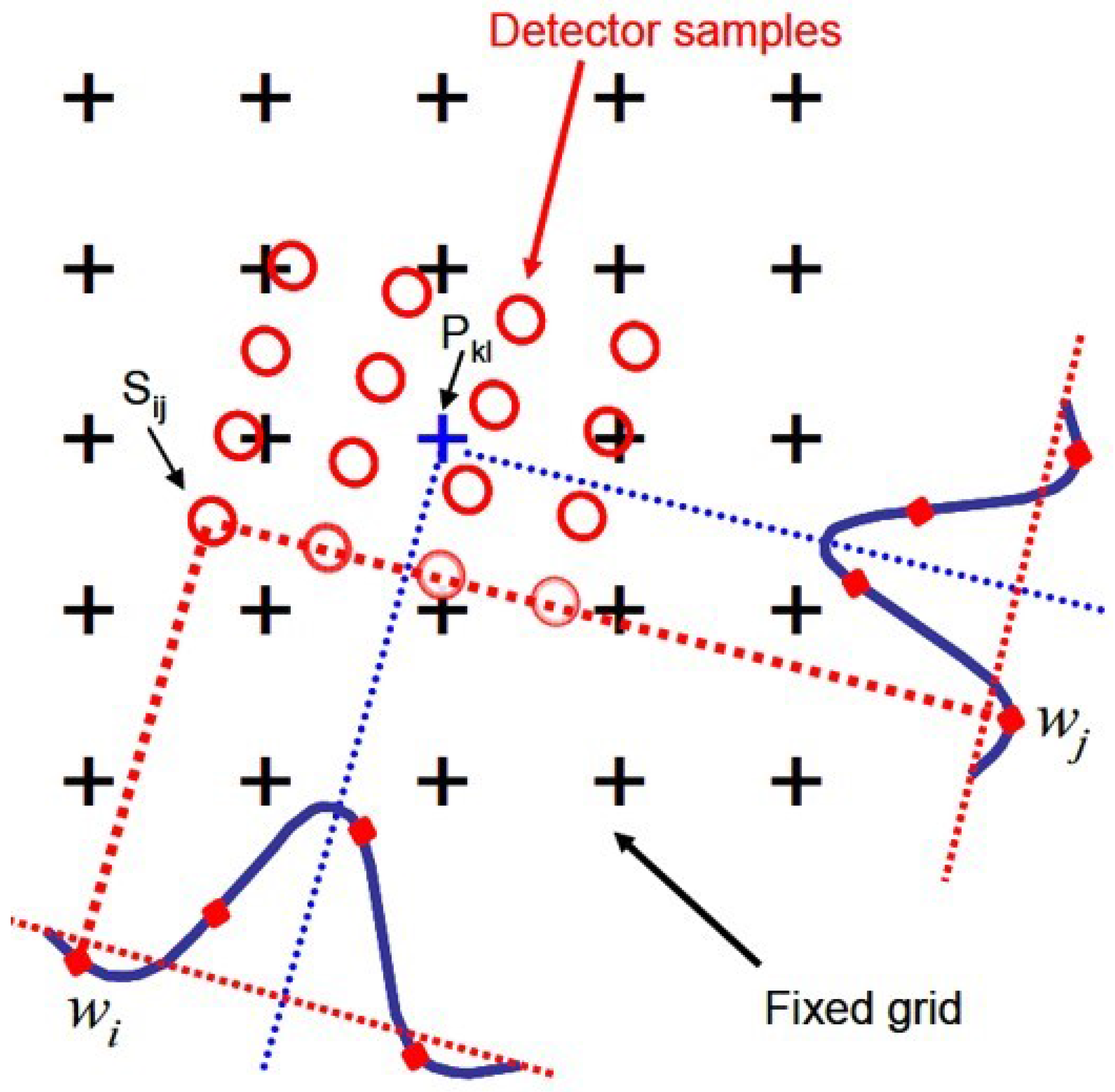
• Calibrated and navigated values are re-sampled to form pixels
• Images are generated in the GOES fixed grid angular coordinate projection

The ground system continuously receives and processes the ABI data into radiances, imagery, and several higher level products that provide geophysical measurements of the land, oceans, and atmosphere for operational meteorology. This paper will describe ABI imaging capabilities and how the sensor data are processed into Level 1B (L1B) radiances within the ground system.

2. ABI Data Collection Approach and Operations

There are three major components of ABI that work together to collect observations of the Earth, space, and calibration targets as a system. These are the scanning mirrors, the Four Mirror Anastigmat (FMA) telescope, and the Focal Plane Modules (FPMs) (Figure 2).

There are two scan mirrors (Figure 3)—one controlling north–south (NS) line-of-sight (LOS) and the other controlling east–west (EW) LOS. They operate independently and simultaneously to slew rapidly to the location of interest and then accurately scan the Earth (or any other scene of interest such as the Moon). As shown in Figure 3, the Earth image is collected in 22 swaths (vs. 1356 swaths for the GOES I/P Imager). The swaths are scanned west-to-east and stepped north-to-south. Each swath has several frames, and the number of frames in a swath depends on the swath duration. A full disk image of the Earth has 22 swaths, where each swath is of a different duration. The swath duration in a full disk image increases from the poles to the Equator since ABI is imaging the Earth’s sphere. The swaths of a full disk are therefore smaller at the poles and contain less frames, compared to the swaths at the Equator. There are six swaths of equal duration and two swaths of equal duration that are used to image the CONUS and mesoscale images, respectively (

Table 2. The number of frames per swath and the swath duration.

Swath	Duration (s)	Frames per Swath
		0.5-km	1-km	2-km
Full Disk: Swath 0	6.750	15,008	7504	3752
Full Disk: Swath 1	8.710	19,360	9680	4840
Full Disk: Swath 2	10.104	22,464	11,232	5616
Full Disk: Swath 3	11.172	24,832	12,416	6208
Full Disk: Swath 4	12.011	26,688	13,344	6672
Full Disk: Swath 5	12.672	28,160	14,080	7040
Full Disk: Swath 6	13.185	29,312	14,656	7328
Full Disk: Swath 7	13.568	30,144	15,072	7536
Full Disk: Swath 8	13.834	30,752	15,376	7688
Full Disk: Swath 9	13.991	31,104	15,552	7776
Full Disk: Swath 10	14.041	31,200	15,600	7800
Full Disk: Swath 11	14.041	31,200	15,600	7800
Full Disk: Swath 12	13.991	31,104	15,552	7776
Full Disk: Swath 13	13.834	30,752	15,376	7688
Full Disk: Swath 14	13.568	30,144	15,072	7536
Full Disk: Swath 15	13.185	29,312	14,656	7328
Full Disk: Swath 16	12.672	28,160	14,080	7040
Full Disk: Swath 17	12.011	26,688	13,344	6672
Full Disk: Swath 18	11.172	24,832	12,416	6208
Full Disk: Swath 19	10.104	22,464	11,232	5616
Full Disk: Swath 20	8.710	19,360	9680	4840
Full Disk: Swath 21	6.750	15,008	7504	3752
CONUS: All swaths	7.114	15,808	7904	3952
Mesoscale: All swaths	2.530	5632	2816	1408

).

The collected photons from the mirrors are imaged by the telescope onto the three focal plane modules: Visible-Near Infrared (VNIR, 0.47 µm to 2.25 µm), Mid-wave IR (MWIR, 3.9 µm to 8.5 µm) and Longwave IR (LWIR, 9.61 µm to 13.3 µm). To obtain a high degree of radiometric precision across the specified dynamic range of observations, the MWIR and LWIR FPMs are cooled to 60 K, and the VNIR FPM is cooled to 180 K (170K for all subsequent flight models).

Each focal plane module (FPM) consists of either five or six individual detector arrays (referred to as focal plane arrays), each of which collects the image in one of ABI’s sixteen bands. The number of rows and columns of detector elements varies by wavelength (Table 1). There are 77,400 detector elements (combination of Side 1 and Side 2 detector arrays), of which 7856 are selected to be read out and downlinked for the operational side—one detector element per row. The selection of which detector element to read out for each row is known as Best Detector Select (BDS). BDS is performed during post launch test once the focal plane arrays have been cooled and then used for the mission. It can be updated at any point by commands from the ground system during the mission life if NOAA determines a selected detector element has ceased to deliver an acceptable output.

Unlike the Imager on the legacy GOES satellites that scans the Earth in a boustrophedonic (“as the ox plows”) manner, the baseline ABI operation scans the Earth in a raster fashion, which results in a higher quality of images due to the constant time interval across swath boundaries (Figure 4). This raster scanning pattern ensures that the time difference between the collection of the southern-most pixel of one swath and the adjacent northernmost pixel of the next swath is the same everywhere along that swath boundary. Thus, if a cloud is moving across the swath boundary, the temporal shift will be identical for all parts of the cloud at the swath boundary. With a boustrophedonic scan pattern, each part of the cloud would have a different temporal shift at the swath boundary, which could distort the shape of the cloud. For the 5-min Full Disk timeline, a boustrophedonic scan pattern would yield a time shift across the swath boundary varying from 0.3 s at one end to 28 s at the other end. It should be noted that, while the baseline is west-to-east raster scans, ABI is capable of scanning in any direction or pattern—e.g., east-to-west raster, east–west boustrophedonic, at an angle, and even purely a north–south scan, which are useful for evaluations of certain on-orbit performance such as detector uniformity.

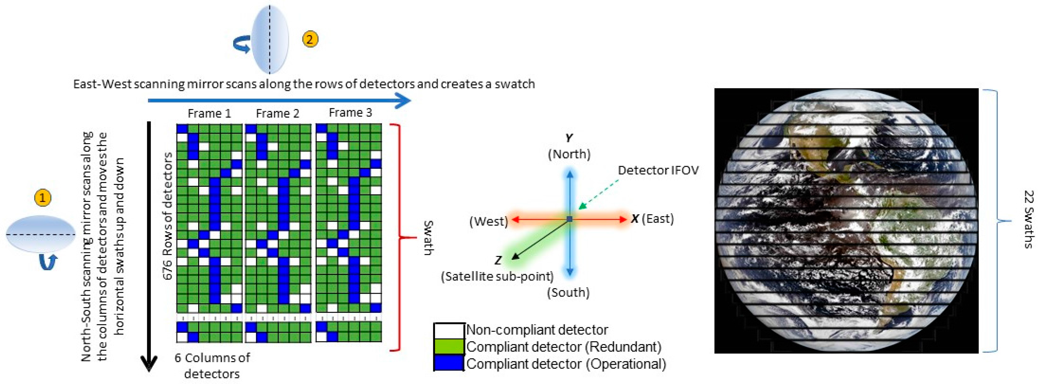
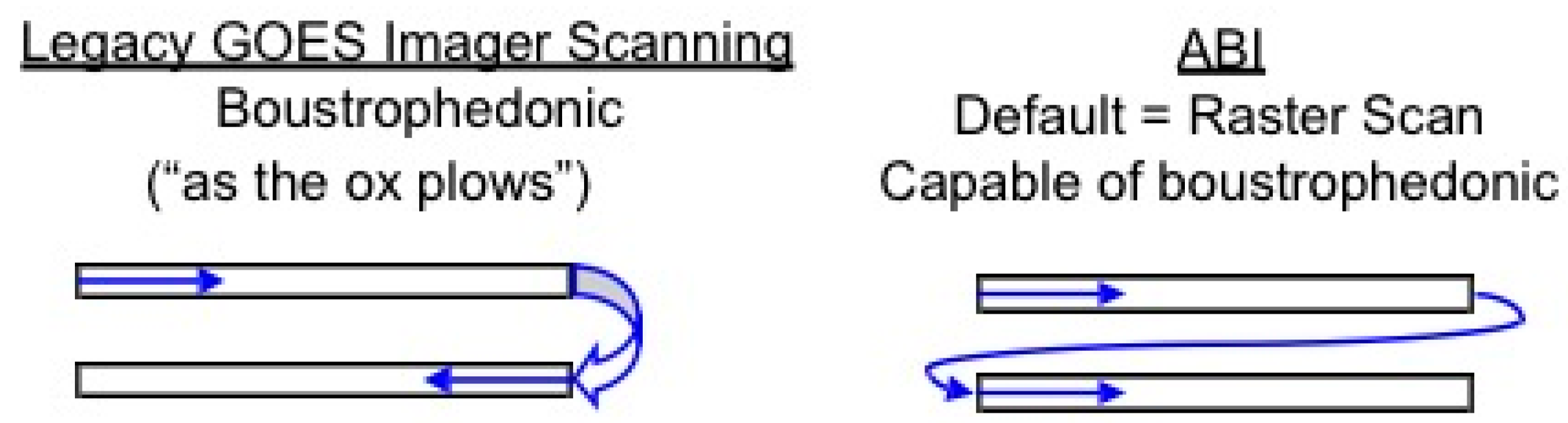
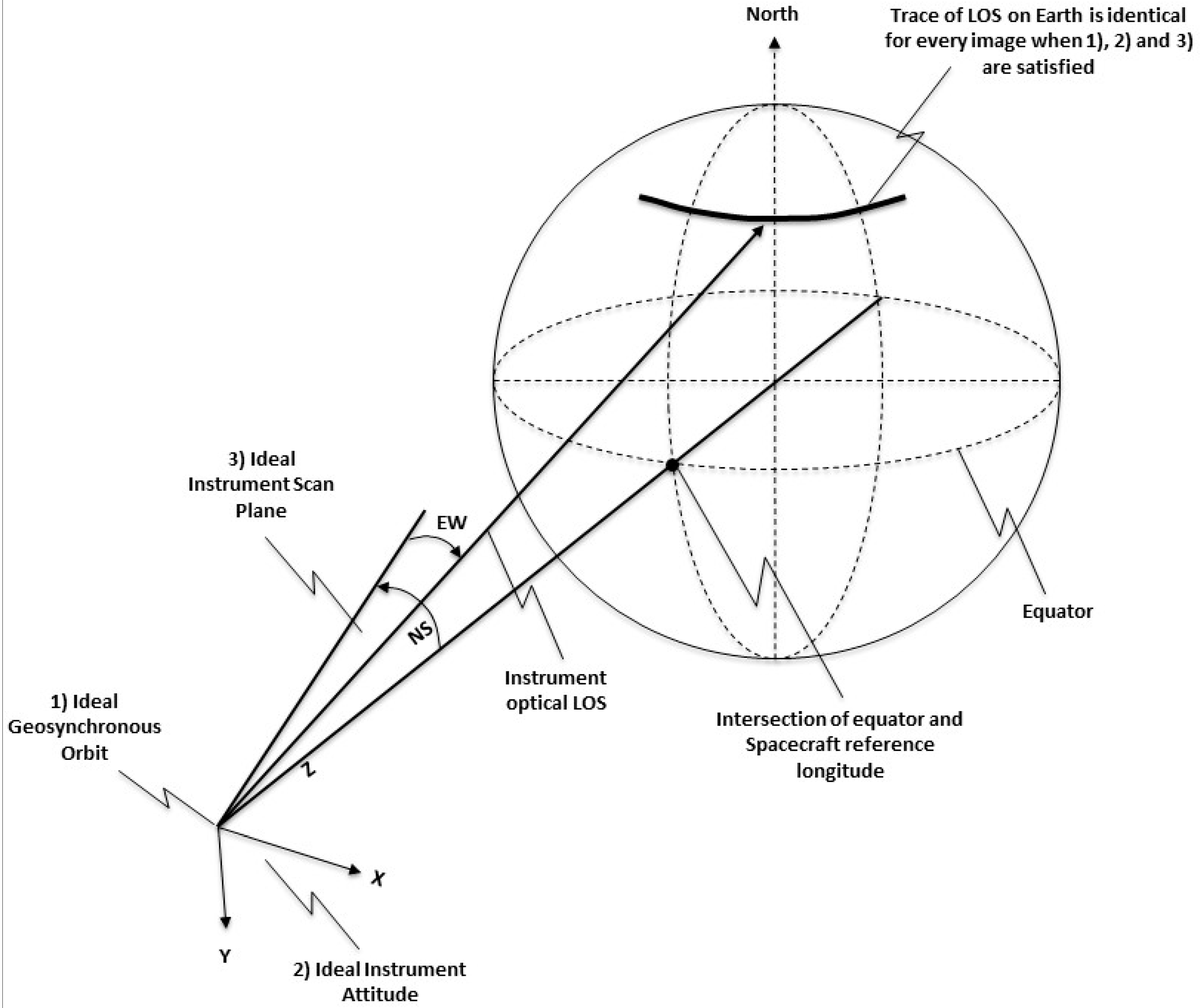
2.1. Observation of the Earth

The ABI baseline scan rate is 0.024434 rad/s (1.4°/s) and the instrument samples the radiance (specifically, the band average spectral radiance) of the Earth in sixteen spectral bands using several arrays of detectors at 14-bit quantization. For Earth scenes, the least significant bits are discarded since they are typically pure noise. This is done to achieve compression efficiency without sacrificing radiometric fidelity to minimize the overall data rate. For each band, the number of bits downlinked (11 to 14) is chosen such that the value of the least significant bit downlinked is less than half the maximum permitted Noise-Equivalent change in Radiance (NEdN) for that band (Table 1). This means that, for a scene of nominal radiance (100% albedo or 300 K), quantization noise is not the dominant contributor to Signal to Noise Ratio (SNR) or Noise-Equivalent delta Temperature (NEdT) (unless the actual SNR or NEdT is significantly better than the requirement). The 100% albedo specified for the reflective bands of ABI is given in

Table 3. The 100% albedo at the nominal center wavelengths of ABI.

Band (μm)	100% Albedo Radiance (mW/m2/sr/cm−1)
0.47	14.4
0.64	21.1
0.86	22.8
1.38	21.7
1.61	20.0
2.25	12.1

.

For calibration scenes, the full 14-bit resolution is downlinked. These scenes are very uniform and compress very well, meaning 14-bit data easily fit within ABI’s downlink allocation. ABI has significantly lower NEdT compared to legacy GOES imager bands, and the actual post launch values are lower than the specification, which allows measurement of the spectral radiances with higher accuracy and precision (Figure 5). A smaller NEdT indicates better performance.

2.2. Observing Stars for Image Navigation and Registration

Within a timeline, ABI makes observations of stars from a predetermined catalogue. The catalogue contains a list of known stars that have sufficient irradiance to yield useful data and are potentially within the ABI Line Of Sight (LOS) at some time during the year. Within a timeline, a star is scanned in the 0.64 μm band on average at least every 100 s and one in the 3.9 μm band is scanned on average every 300 s. The ground system calculates the optimum stars to observe during every 2.5-min time interval and uploads that table to ABI on at least a weekly basis. When a timeline specifies the collection of a star image, the ABI flight software looks up the identification number of the best star from this table, finds the location of that star in the onboard star catalog, and then calculates where the star will be located at the time of the observation. This information is used to point the ABI LOS to scan that location. Star observations are used in the Image Navigation and Registration (INR) algorithms as described later in Section 3.3.

2.3. Observing the Onboard Calibration Targets

ABI has two onboard calibration targets: a blackbody for emissive bands, referred to as the Internal Calibration Target (ICT); and a solar diffuser for the reflective bands called the Solar Calibration Target (SCT) that is made of Spectralon^®. The ICT is observed at the beginning of every timeline, whereas the SCT is observed less frequently (because the change in calibration of the VNIR bands is far slower than that of the LWIR). The SCT is protected from degradation due to UV radiation and molecular contamination by the solar calibration cover (SCC), which is opened only when the SCT has to be exposed to the sun during calibration events. The SCT is viewed frequently (e.g., every two days) during the first years after launch, but is gradually changed to quarterly observations after the radiometric calibration is well characterized.

2.4. Observations of Space

Within a given timeline, ABI periodically makes observations of space to provide the background measurement for both the emissive and reflective radiometric calibrations. Space observations occur at least every 30 s. These frequent space observations ensure that the calibration accuracy requirements are met, while the redundancy allows any corrupted space looks to be discarded without impacting data products. Observations of space and the calibration targets are used to convert the digital counts from the detector samples into calibrated radiances (more on this in Section 3.2).

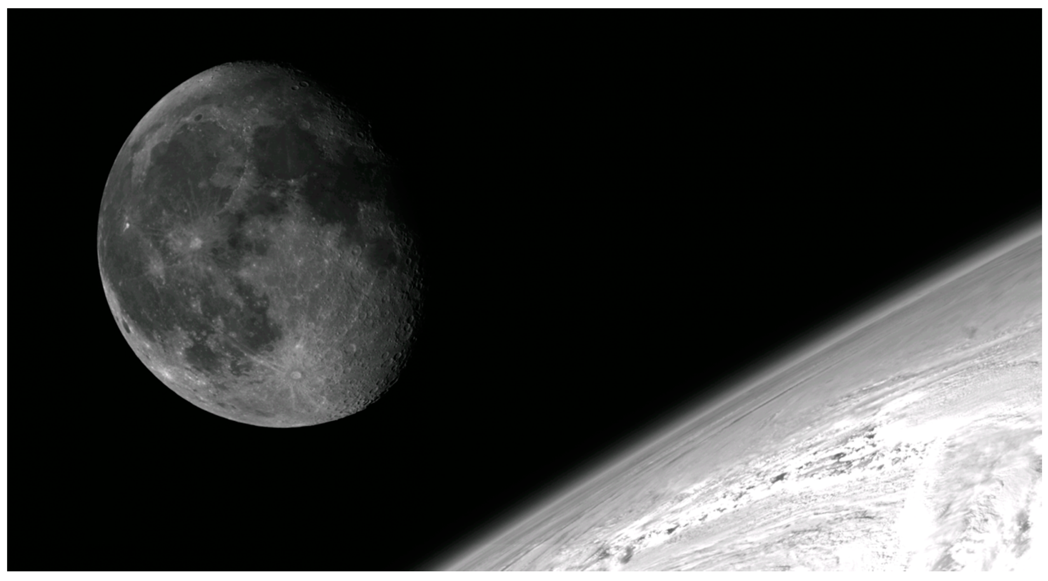
2.5. Observations of the Moon

Unlike onboard calibration targets that degrade over time or Earth surface targets that are used for vicarious calibration, the Moon is a very stable reflector and views of the Moon by satellite sensors have been used for long term characterization [4]. First, ABI can collect several Moon images without impacting the core image collections of Full Disk and CONUS. During the standard observation timeline (Scan Mode 3), the time slot allocated to collection of 30 s Mesoscale images can be repurposed to observe the moon. The height of the Moon is approximately 40% of the ABI swath height, which means only a single swath is required to observe the entire Moon, which permits many such images to be collected each time the Moon passes through the ABI field of regard (Figure 6). Many images with similar phases of the Moon can be used to reduce uncertainties in the evaluation of each individual image.

The ability to scan the entire Moon in a single swath also drastically reduces one significant error source in using the Moon for characterization—knowledge of where on the Moon each detector sample was collected. With the complete image of the Moon in a single swath, the north, south, east, and west edges can be clearly identified, which permits every detector sample to be precisely registered to the lunar surface. The World Meteorological Organization (WMO), through the Global Space-based Inter-Calibration System (GSICS) [5], coordinates international collaboration to develop a standard methodology for vicarious calibration of satellites instrument using lunar irradiance. ABI is particularly well suited for such an approach.

3. Ground System Processing

The ABI samples (detector counts) are compressed, formatted into data packets (packetized), and downlinked to the ground station (Level 0 data) for conversion to calibrated, geo-located pixel images (Level 1b data). The detector samples must be decompressed, radiometrically calibrated, navigated, and resampled to produce pixels that are located on an invariant output grid, referred to as the fixed grid. Each of these processes are described below.

The following definitions are used to define various data types in processing sensor data from ABI:

• Raw Data: Data in Consultative Committee for Space Data Systems (CCSDS) protocol transfer frames, as received from the satellite.
• Level 0 Data: Reconstructed unprocessed instrument data at full resolution; and all communications artifacts (e.g., synchronization frames, communications headers) removed.
• Level 1a Data: Level 0 data with all supplemental information appended for use in subsequent processing.
• Level 1alpha Data: Calibrated detector samples in radiance units in a swath but not navigated.
• Level 1beta Data: Calibrated detector samples in a swath, with detector rows aligned, navigated but not resampled.
• Level 1b Data: Calibrated and navigated detector data resampled into pixels in the fixed grid.

3.1. Level 0 Data Processing

ABI data are downlinked in packets that conform to the CCSDS Space Packet Protocol standards (CCSDS recommendation 133.0-B-1) [6] and utilize lossless data compression to fit within the allocated bandwidth. The ground system terminal consists of an antenna, a suite of equipment to process Radio Frequency signals into a digital data stream, and software to process extracted CCSDS packets. Forward error correction (FEC) is used to minimize risk of data loss due to link errors and allow for verification of data integrity within the ground system data reception equipment.

Level 0 data processing starts with the ingest of CCSDS packets. Each CCSDS packet has a primary header which includes an Application ID (APID) that is unique to each packet type. The APID is used to distinguish the type of data in the packet. For instance, there is a separate APID for each band of science data. After decompressing the contents of these packets, the data are reordered back into the swaths from which they originated. The first step is arranging packets back into data chunks using metadata within each packet.

Every four packets of channel data comprise a data chunk. A data chunk is a collection of eight consecutive detector samples in a single swath from all active columns of a given band. Many detector samples make a swath, and one or more swaths make a scene (Figure 7). Rice compression is done across the rows within the chunk, and then the compressed rows are assembled into packets with every fourth compression block gathered into one packet. ABI uses a 4 × 4 resampling kernel so the loss of a single packet will not result in a hole in imagery but rather slightly degraded radiometric accuracy.

As Level 0 processing software module collects packets, it decompresses the data and stores the samples in Level 1a data blocks. L1a data blocks are a grouping of consecutive detector columns, i.e., many data chunks, within a single swath (Figure 8). As L1a data blocks are filled, they are sent onwards for Level 1 Processing.

Aside from channel imagery, other scene types processed include Spacelooks, Solar Calibration Targets (SCT), Infrared Calibration Targets (ICT), as well as stars. These scenes are used to radiometrically calibrate and navigate the channel imagery.

In conjunction with creating L1a data blocks, Level 0 also archives all packets received. These files can be used for analysis, anomaly resolution, and even playback through the system.

3.2. Radiometric Calibration

The GOES-R Ground Segment implements the radiometric calibration of the ABI Thermal Emissive Bands (TEB) and Reflective Solar Bands (RSB) as a collection of algorithms for processing the blocks of ABI detector data generated by the L0 Processing subsystem after the decompression and assembly of the telemetry packets. These ground processing calibration algorithms achieve on-board SI metrological traceability using a blackbody source with an emissivity of better than 0.995 called the Internal Calibration Target (ICT) for TEB calibration and a Spectralon^® diffuser called the Solar Calibration Target (SCT) for RSB calibration [7]. The ABI instrument uses these calibration targets together with a space view collected every 30 s to determine the background count level from the instrument optics and electronics at zero radiance. Although the ABI instrument is also capable of collecting many additional types of calibration scenes because of its unique scan flexibility [8], the current set of operational algorithms in the ground system are not designed to ingest and use these data in the present configuration. However, the ground system does provide the telemetry packet data for these calibration scenes for offline processing by the GOES-R calibration and validation team.

To meet the latency requirements for the L1b Radiance product, the ground system uses a set of algorithms, optimized for the system architecture design, for processing a block of detector data from each scene type, including space looks, ICT, SCT, star looks, and the Earth view scanning modes of full disk, CONUS, and mesoscale. The ABI calibration algorithms are similar to those for the Advanced Himawari Imager (AHI) on the Himawari-8 geostationary satellite of the Japan Meteorological Agency (JMA, Tokyo, Japan) [9] because of the similarities in the instrument design.

For each calibration scene, the ground system executes the appropriate calibration algorithm as soon as L0 Processing makes the appropriate scene available, updating the associated parameters used to calibrate Earth scene data. Each Earth scene detector sample is calibrated as soon as it is received, using the latest values for all of the calibration parameters. The L1b calibration algorithm then retrieves the required auxiliary input data for processing, including ABI engineering telemetry and semi-static algorithm processing parameters, based on the starting and ending times of the scene data. Each radiometric calibration algorithm generates an intermediate data product that serves as input for either another radiometric calibration algorithm or a navigation algorithm. The outputs of the calibration algorithm are referred to as L1-alpha intermediate products; the final L1b Radiance product is the result of subsequent processing by the image navigation (producing L1-beta) and resampling algorithms (producing L1b).

Calibration parameters used by the L1b software are maintained as database files in easy-to-maintain HDF (or xml) format. These parameters were updated for launch and revised during the PLT phase, and will be updated as needed during the life of the program.

3.2.1. Space Looks (Observations of Space)

The ABI L1b space look algorithm determines the offset in the measured digital number (DN) counts from the space look scene data. There are two types of space looks: (1) routine space look ($x_{sp})$ configuration consisting of 64 samples at the beginning of each 30-s swath for each of the Earth-observing timelines; and (2) Solar calibration space looks ($x_{SCT})$ that are only observed during solar calibration timeline consisting of 256 samples. Both the two space looks are calculated and used separately in the calibration.

The main function of the space look algorithm is to compute the average offset in counts ${\overline{x}}_{sp}$ for each detector in the current band and data path. Before computing this average, the algorithm first checks the space look detector samples for saturation and removes outlier values. In addition, the algorithm also computes the spectral radiance differences between each sample and the previous space look measurement for the detector to determine if the samples are contaminated by the moon being in the instrument field of view. For detectors failing these tests, the algorithm propagates the previous average offset for the current detector.

All of the radiometric calibration algorithms compute the reflectivity for the North–South $({\rho }_{NS})$ and the East–West $({\rho }_{EW})$ scan mirrors using the mirror shaft angles from the ABI engineering telemetry. The algorithm uses semi-static parameter look-up tables measured before launch to determine the angular dependence of the reflectivity. For TEB data blocks, the algorithms also compute the emissivity of the North–South $({\epsilon }_{NS})$ and East–West (${\epsilon }_{EW}$) of the scan mirrors from their reflectivity as follows:

$${\epsilon }_{NS}=1-{\rho }_{NS}$$

(1a)

$${\epsilon }_{EW}=1-{\rho }_{EW}$$

(1b)

The space look algorithm determines the effective self-emission, band-averaged spectral radiance for the NS and EW scan mirrors to account for their contribution to the calibration. The algorithm uses the average temperature computed from the scan mirror thermistor values in the ABI engineering telemetry to determine the channel averaged emitted radiance for the North–South $\langle L_{NS}\rangle$ and East–West $\langle L_{EW}\rangle$ mirrors at this temperature from measurements made pre-flight. The algorithm then computes the effective radiances for the scan mirrors from the following expressions:

$$L_{NS}^{eff}=\langle L_{NS}\rangle {\epsilon }_{NS} {\rho }_{EW}$$

(2a)

$$L_{EW}^{eff}=\langle L_{EW}\rangle {\epsilon }_{EW}$$

(2b)

where $L_{NS}^{eff}$ is the effective radiance for the North–South scan mirror and $L_{EW}^{eff}$ is the effective radiance for the East–West scan mirror.

3.2.2. Thermal Emissive Band Calibration

The ICT algorithm uses the ICT scene data together with the most recent intermediate space look algorithm output to compute the gain coefficients for each detector of the current TEB. After calculating the scan mirror effective radiances, the algorithm computes the ICT emitted radiance from the average ICT temperature of the attached platinum resistance thermometer sensor values in the ABI engineering telemetry and the pre-flight look-up table, and determines the effective radiance $(L_{ICT}^{eff})$.

$$L_{ICT}^{eff}=\langle L_{ICT}\rangle {\epsilon }_{ICT} {\rho }_{NS@ICT} {\rho }_{EW@ICT}$$

(3)

where,

• $\langle L_{ICT}\rangle$ is the channel averaged spectral radiance of the ICT;
• ${\epsilon }_{ICT}$ is the channel specific emissivity of the ICT; and
• ${\rho }_{NS@ICT}$ and ${\rho }_{EW@ICT}$ are North–South and East–West mirror reflectivities respectively at the time of ICT measurement.

The ICT algorithm next computes the linear gain coefficient for each detector in the current emissive band that is not flagged in the dead row list, which is updated periodically on-orbit. The IR gain coefficient $m_{IR}$ computation depends on the effective radiances for the scan mirrors and the ICT computed for the ICT scene time and the most recent space look, the difference between the average ICT and space look counts $(\Delta x_{ICT}={\overline{x}}_{ICT}-{\overline{x}}_{sp})$ to remove background contributions, and the non-linear, quadratic coefficients $Q$, determined pre-launch for each detector of each band.

$$m_{IR}=\frac{L_{ICT}^{eff}+(L_{NS@ICT}^{eff}+L_{EW@ICT}^{eff})-(L_{NS@sp}^{eff}+L_{EW@sp}^{eff})-Q{(\Delta x_{ICT})}^2}{\Delta x_{ICT}}$$

(4)

Since the ABI instrument observes the ICT at the start of every Earth viewing timeline, the IR gain coefficient is updated at least every 15 min. For detectors flagged by the dead row list, the algorithm sets both the linear and the quadratic gain coefficients to zero to ensure that bad values of the radiance are not propagated to the downstream processing. In addition, the algorithm also sets a quality flag to indicate a bad value for the particular detector.

The IR radiance retrieval algorithm computes the Earth scene radiance for each sample of each detector for the current TEB. This calibration equation implemented by the algorithm for converting the measured counts for a sample to the band-averaged spectral radiance is a function of the difference between the detector sample and the space look average $(\Delta x_{smp}=x_{smp}-{\overline{x}}_{sp})$:

$$L_{smp}=\frac{m_{IR}\Delta x_{smp}-(L_{NS@smp}^{eff}-L_{NS@sp}^{eff})-(L_{EW@smp}^{eff}-L_{EW@sp}^{eff})+Q{(\Delta x_{smp})}^2}{{\rho }_{NS@smp} {\rho }_{EW@smp}}$$

(5)

where,

• $\langle L_{smp}\rangle$ is the radiance of the sample;
• $L_{NS@smp}^{eff}$ is the channel average effective radiance for the North–South scan mirror when the samples were collected;
• $L_{EW@smp}^{eff}$ is the channel average effective radiance for the East–West scan mirror when the samples were collected;
• $L_{NS@sp}^{eff}$ is the channel average effective radiance for the North–South scan mirror when the space looks were collected; and
• $L_{EW@sp}^{eff}$ is the channel average effective radiance for the East–West scan mirror when the space looks were collected.

The algorithm also generates a 1-bit quality flag indicating the status of the sample radiance by comparing the value with under-saturation and over-saturation thresholds based on pre-flight measurements. These quality flags are also used by the resampling algorithm to determine the L1b product pixel quality flags. The algorithm computes the TEB radiances in units of $\mathrm{mW}/({\mathrm{m}}^2 {\mathrm{sr}\mathrm{cm}}^{-1})$.

3.2.3. Reflective Solar Band Calibration

For RSB radiometric calibration, the SCT algorithm computes the visible and infrared (VNIR) gain coefficient using the SCT scene data collected during the solar calibration timeline. This timeline, which is only used for calibration and contains no Earth scene data, is scheduled as needed to limit degradation of the SCT. At the start of the mission, the solar calibration was done every two days and then changed to once a quarter for the rest of the mission lifetime.

The SCT algorithm first computes the average SCT counts after outlier removal, and the scan mirror reflectivities. The algorithm computes the SCT band-averaged spectral radiance $\langle L_{SCT}\rangle$ from the following equation:

$$\langle L_{SCT}\rangle =K_{{\beta }_{eff}}^{detector row \#} \cos ({\theta }_{sun}) \left[\pi \langle L_{100\%\alpha }\rangle {(\frac{R_{sun}}{r_{sun}})}^2\right]$$

(6)

where,

• $R_{sun}$ is the average distance from the Sun to the Earth;
• $r_{sun}$ is the actual distance between the Sun and the Earth at the time of the measurement;
• $\pi \langle L_{100\%\alpha }\rangle$ is the solar irradiance at 1 AU over a Lambertian surface with 100% albedo; and
• ${\theta }_{sun}$ is the Sun-to-SCT diffuser normal angle of incidence.

The factor $K_{{\beta }_{eff}}^{detector row \#}$ is related to the effective bidirectional reflectance distribution function of the solar calibration target and is determined pre-flight. The algorithm uses $\langle L_{SCT}\rangle$ with the scan mirror reflectivities to determine the effective band-averaged spectral radiance of the SCT $L_{SCT}^{eff}$.

$$L_{SCT}^{eff}=\langle L_{SCT}\rangle {\rho }_{NS@SCT} {\rho }_{EW@SCT}$$

(7)

where, ${\rho }_{NS}$ and ${\rho }_{EW}$ are the reflectivities of the North–South and East–West mirrors, respectively, when the SCT was observed.

The SCT algorithm computes the linear VNIR gain $m_{VNIR}$ for each detector in the current solar reflective solar band that is not flagged in the dead row list. The VNIR gain coefficient computation depends on the effective radiance of the SCT, the difference between the average SCT and solar space look counts $(\Delta x_{SCT}={\overline{x}}_{SCT}-{\overline{x}}_{ssp})$, and the non-linear, quadratic coefficients $Q$, determined pre-launch for each detector of each band.

$$m_{VNIR}=\frac{f_{int,ch}{L}_{SCT}^{eff}-Q{(\Delta x_{SCT})}^2}{\Delta x_{SCT}}$$

(8)

This equation includes an additional integration factor $f_{int,ch}$ for each band determined pre-launch to account for the change in integration time to measure a higher signal. This equation is similar to that for computing the IR gain coefficients except that the scan mirror radiances are set to zero. As for the TEB calibration, the algorithm sets both the linear and the quadratic gain coefficients to zero if the detector is flagged by the dead row list and sets the corresponding 1-bit quality flag to bad.

The VNIR radiance retrieval algorithm computes the Earth scene radiance for each sample of each detector for the current RSB. This calibration equation implemented by the algorithm for converting the measured counts for a sample to the band-averaged spectral radiance is a function of the difference between the detector sample and the space look average $(\Delta x_{smp}=x_{smp}-{\overline{x}}_{sp})$ as follows:

$$\langle L_{smp}\rangle =\frac{m_{VNIR}\Delta x_{smp}+Q{(\Delta x_{smp})}^2}{{\rho }_{NS@smp} {\rho }_{EW@smp}}$$

(9)

It should be noted that the noise in downlinked detector samples can increase or decrease the count value. If it decreases the count value, then when the average space look value in counts is subtracted from the downlinked detector sample in counts, a negative difference can result for very low signal levels, which can result in a negative radiance out of Equation (9). The algorithm also generates a 1-bit quality flag indicating the status of the sample radiance by comparing the value with under-saturation and over-saturation thresholds based on pre-flight measurements. The algorithm computes the RSB radiances in units of W/m²/sr/μm.

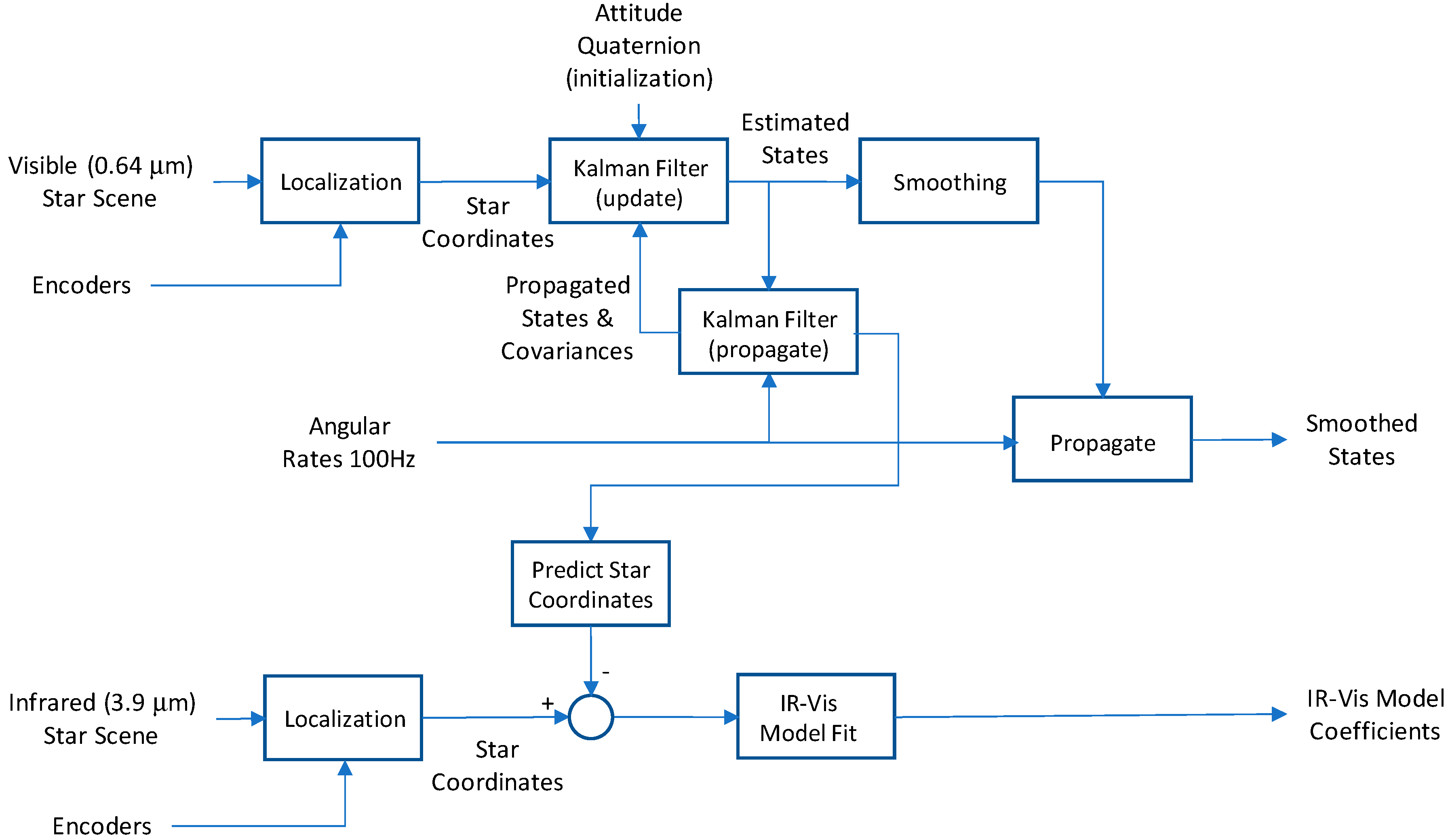
3.3. Image Navigation and Registration

INR for the ABI assures that L1b pixels are accurately registered to a fixed grid for each spectral channel. The ABI fixed grid, which is defined in the Product Users Guide (PUG) [10], is an angle-angle coordinate system representative of an ideal scanning instrument with the origin being the sub-satellite point for an ideally positioned satellite. Figure 9 shows a GOES-16 Full Disk embedded in the fixed-grid coordinate system with the CONUS scene boundary for the reference longitude of the post-launch test location of GOES-16 (89.5°W). The ABI fixed grid is a projection based on the viewing perspective of the idealized location of a satellite in geosynchronous orbit. This allows the same data points in every product to be at the same location on the Earth. The origin of the fixed grid represents the satellite sub-point, which, by definition, is at the coordinates (y = 0, x = 0). The fixed-grid coordinates are specified for the center of each scene.

The coverage associated with the ABI images is defined in terms of the viewing angle of the Earth from the satellite perspective. Note that the term “scene” is used to communicate what the ABI instrument observes. The term “image”, is used to communicate the product data resulting from the scene. East to west and north to south coverage regions of the Earth’s full disk on the fixed grid are 0.303704160 radians and 0.302701402 radians about the satellite’s x and y axis respectively or about ±8.7°, which is the apparent diameter of the Earth from geostationary orbit (Figure 10). The EW and NS fixed-grid coordinates increase by exactly 56 μradians per pixel for each of the 12 spectral channels with a 2-km nadir spatial resolution, by 28 μradians for the three 1-km resolution channels, and by 14 μradians for the single 0.5-km resolution channel. There is an invariant relationship between the fixed-grid coordinates of a pixel center and the geodetic latitude and longitude, where the line of sight from that pixel pierces the GRS80 ellipsoid. The fixed-grid sites at each resolution are selected so that the pixels of higher resolution spectral channels nest inside those of the lower resolution channels (Figure 10). Note that for each of the full disk, CONUS, and mesoscale products, this relationship holds true when the lower resolution data are a multiple of the higher resolution data. The reported radiance for a 2-km pixel is not the average radiance over a 2 km × 2 km area. Rather, it is the best estimate of the radiance at the center of that 2 km × 2 km area.

Figure 11 illustrates this relationship derived from the interpretation of fixed-grid coordinates as idealized scan angles. Deviations in the placement of pixels with respect to the fixed grid given their true geographic coordinates is termed “navigation error”. The stability of image navigation between consecutive frames of the same scene (“frame-to-frame registration”), relative alignment between channels (“channel-to-channel registration”), and the alignment between swaths (“swath-to-swath registration”) are other important measures of INR performance.

According to the GOES-R General Interface Requirements Document (GIRD) [12], the spacecraft provides the following information to allow ABI scene collection:

• Quaternion: ~100 μrad uncertainty (sampled at 1 Hz)
• Attitude rate measurements: <20 μrad drift over 15 min (sampled at 100 Hz)
• Spacecraft position: 35 m in-track, 35 m cross-track and 70 m radial over 15 min (sampled at 1 Hz)
• Spacecraft velocity: <6 cm/s uncertainty per axis (sampled at 1 Hz).

The primary ABI reference frame is J2000, which is the inertial frame used by the star catalog. Star coordinates are rotated into a True of Date frame and then into an Earth Centered Fixed (ECF) coordinate frame with the x-axis oriented to the station longitude. Orbit determination and body axis attitude reporting are done relative to the Orbit Reference Frame (ORF) defined by the velocity vector and nadir. The ABI instrument alignment is referenced to the Instrument Mounting Frame (IMF)—relative to the spacecraft body axis, and the line of sight is referenced to the ABI mounting frame. ABI commanding and image navigation is defined relative to the Fixed Grid Frame (FGF) defined as an ideal GEO orbit located at the GOES east or GOES west station longitude (Figure 11).

INR is implemented on the ground for GOES-R using a Kalman Filter-Smoother [13], which is a different approach than the legacy NOP series. The Kalman Filter has 18 states that represent the attitude of the ABI and a set of internal ABI optical and alignment variables, plus their rates. Figure 12 shows the flow of the INR processing, which relies on star sensing through the aperture of the ABI instrument to determine the ABI attitude with respect to the fixed grid. Visible channel (band 2, 0.64 μm) stars are scanned during the execution of a timeline and the Kalman Filter updates its estimated state after each star sighting. In between star sightings, the state is propagated using inertial attitude rate measurements derived from a high-performance inertial reference unit flown with the ABI and included in the ABI telemetry [14]. Spacecraft orbit is determined onboard by a GPS navigation system, and angular encoder data for each of the two scan mirrors are also included in the ABI telemetry stream.

Together, the Kalman Filter states, orbital position, and encoder output at any instant, plus a map of the active detectors are all that would be required to navigate the detector samples for band 2. However, sliding-window weighting of the state update steps is used to compute “smoothed” states for sample navigation purposes. The smoothed (rather than filter) states are used to navigate the band-2 detector samples so that swath-to-swath registration error is minimized between updates. Navigation of the IR channels requires an additional correction for misalignments between band 2 and band 7 (3.9 μm), which change diurnally as thermal conditions change on orbit. IR stars from band 7 are scanned during each timeline and a 30-h sliding window of such measurements is used to derive a polynomial model for the alignment between the VNIR and MWIR focal plane assemblies. This is different than the more immediate processing of band-2 stars, which are directly input into the Kalman Filter-Smoother. The smoothed states derived from band-2 star measurements are used to define optical pointing of the VNIR (bands 1–6) focal plane center. The MWIR-VNIR misalignment correction computed from band 7 stars is used to define the optical offset of the MWIR and LWIR centers with respect to the VNIR center. Relative Detector Position tables define the optical positions of the individual detectors relative to the optical center for each band.

Creating the L1b pixels in the fixed-grid is the last step in INR. The pixels for the L1b product are resampled from the calibrated and navigated detector samples in a pipelined process as blocks of calibrated and navigated detector samples flow through the system. The “Resampler” algorithm is designed to minimize the time to deliver pixels to be broadcast in the GOES-R Rebroadcast (GRB) and optimize overall product latency. There is a distinction between detector samples and products pixels, and note that the spatial sampling by the ABI detectors is finer than the pixel resolution of the ABI products (Table 1). In general, a pixel p at each fixed-grid coordinate that belongs to an ABI product is formed as a weighted combination of a 4 × 4 matrix of samples as shown in Figure 13. Each detector sample ($s_{i,j}$) is navigated individually and the weights ($w_i, w_j)$ assigned to that sample are based on the resulting distance of the sample from the pixel p.

$$p=\frac{{\displaystyle {\sum }_{i=0}^3}{\displaystyle {\sum }_{j=0}^3}{w}_i{w}_j{s}_{i,j}}{{\displaystyle {\sum }_{i=0}^3}{\displaystyle {\sum }_{j=0}^3}{w}_i{w}_j}$$

(10)

All contributing samples come from the same swath. The scanning of the swaths in space will closely but not perfectly match the swath of the L1b imagery to be distributed in GRB and it is therefore necessary for all but the first swath to mosaic a small fraction of resampled pixels from the prior swath together with those of the current swath to build a full swath of GRB. The transition line between those pixels from the current scan swath and those from the previous scan swath is called the “arbitration” line. The arbitration line is drawn so that it is consistent across all channels, i.e., all higher resolution pixels within a lower resolution pixel come from the same scan swath. Pixels very close to the top or bottom of a swath could be constructed from fewer than 16 samples, but such pixels generally fall on the wrong side of the arbitration line and are not included in the product. In practice, almost all pixels are formed from 4 × 4 samples and those formed from 12 or fewer would be assigned a data quality flag indicating “conditional use”.

INR performance is operationally monitored by the Product Monitoring (PM) tool, which matches image features at landmark sites to a digital map created from the Shuttle Radar Topographic Mission (SRTM) Water Body Data [15], and performs tie-point matches under clear skies to measure frame-to-frame offsets. The PM landmarks are located at predefined sites where land-water boundaries are present and stored in a configuration controlled catalog. INR performance for the GOES-R system meets the requirements with margin. Figure 14 shows an example from PM of the metrics for navigation error and frame-to-frame registration queried from the operational system just after its INR parameters were tuned and before GOES-16 was transitioned into operations at its permanent station in orbit.

On 10 July 2017, the calibrated and geo-located (i.e., Level 1b) data of ABI onboard GOES-16 were released to the public with “Provisional” maturity. Provisional data are defined as a product that is ready for operational use with any known issues documented; the known issues are expected to be fully resolved before the products are declared “Validated”. Prior to the release, the GOES R-Series (GOES-R) Calibration Working Group (CWG) assessed the geometric calibration (INR) of GOES-16 ABI by comparing the ABI imagery with landmarks. The landmarks are created from Landsat-8 observations of corresponding channels with resolution of 30 m. These observations are remapped onto the fixed grid for the planned ABI viewing positions (75°W for GOES-East, 137°W for GOES-West, and 89.5°W for Checkout), using a Digital Elevation Map with resolution of 90 m. The landmarks are downsampled and ABI image is interpolated to an intermediate resolution for comparison. The pair of ABI image fragment and landmark must satisfy several criteria of good viewing conditions. Result of correlation (navigation residuals) must also pass a series of filters. These filtered residuals are then analyzed with standard statistical methods to produce the metrics for evaluation of requirements compliance. INR metrics that are evaluated include image navigation residuals, channel-to-channel registration, swath-to-swath registration, within-frame registration, and frame-to-frame registration. Based on this substantial but preliminary analysis of ABI data since launch, CWG concluded that ABI INR navigation errors of principal bands are within expected values demonstrating the validity of the novel navigation approach (

Table 4. Required, pre-launch estimate (expected), and on-orbit validation of channel navigation errors for GOES-16 ABI. The error is bias plus three standard deviations. EW is East–West direction, NS is North–South direction. INR performance is for the 99.73rd percentile over 24 h (data from the Calibration Working Group, NOAA/NESDIS/STAR).

Navigation Errors of ABI Principal Bands (CWG Evaluation)
Band (µm)	Required (µrad)		Expected (µrad)		Measured (µrad)
	EW	NS	EW	NS	EW	NS
0.64	28.0	28.0	10.4	10.1	3.0	1.2
0.86	28.0	28.0	10.5	10.3	6.0	5.0
2.25	28.0	28.0	10.6	10.4	13.1	10.4
3.90	28.0	28.0	11.4	11.3	12.5	14.3
10.35	28.0	28.0	11.9	12.5	13.8	12.9

).

4. Early Results from ABI

After successful launch of the spacecraft followed by outgassing of ABI, the “first light” full disk and CONUS public images of the Earth were acquired and processed on 15 January 2017, and released to the public on 23 January by NOAA and NASA. Since then, ABI has been transmitting data routinely to the ground stations where the raw data are processed to L1b as described in Section 3, and these data are rebroadcast across the Western Hemisphere as GOES Rebroadcast (GRB). NOAA scientists have been analyzing the data for verification and validation of the products through intense field campaigns where data from ABI is compared with well characterized in-situ measurements and measurements collected from instruments on NASA’s high altitude ER-2 aircraft to characterize the performance of the ABI. The L1b data have reached provisional maturity, meaning that the data are ready for operational use, and the product performance has been demonstrated through analysis of a small number of independent measurements obtained from selected locations, periods, and associated ground-truth/field efforts. The GOES-R ground system has latency requirements to process raw data to L1b in 50 s for full disk and CONUS data collection, and in 23 s for mesoscale; the ground system is able to process the data within these latencies. The ABI imagery is significantly better compared to the legacy GOES Imager because of the improved spectral, spatial and temporal resolution of ABI. Some results of analysis of the sensors radiometric performance and examples from the first year are shown below.

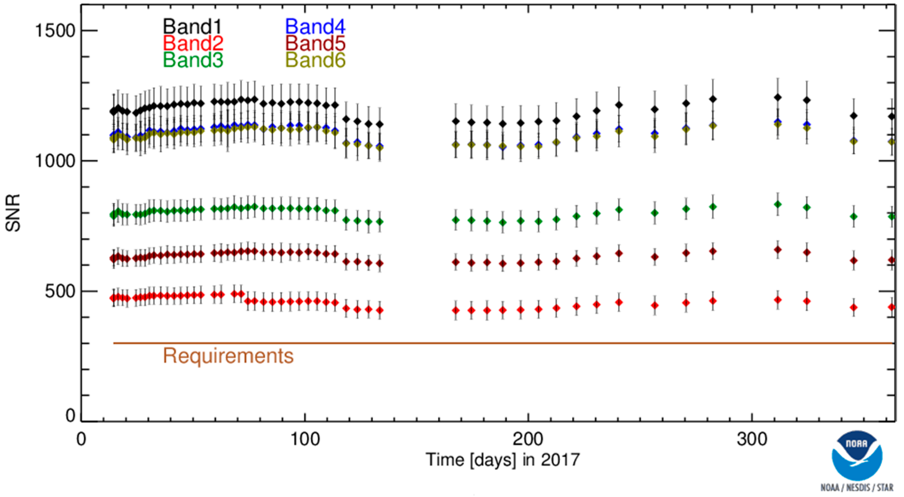
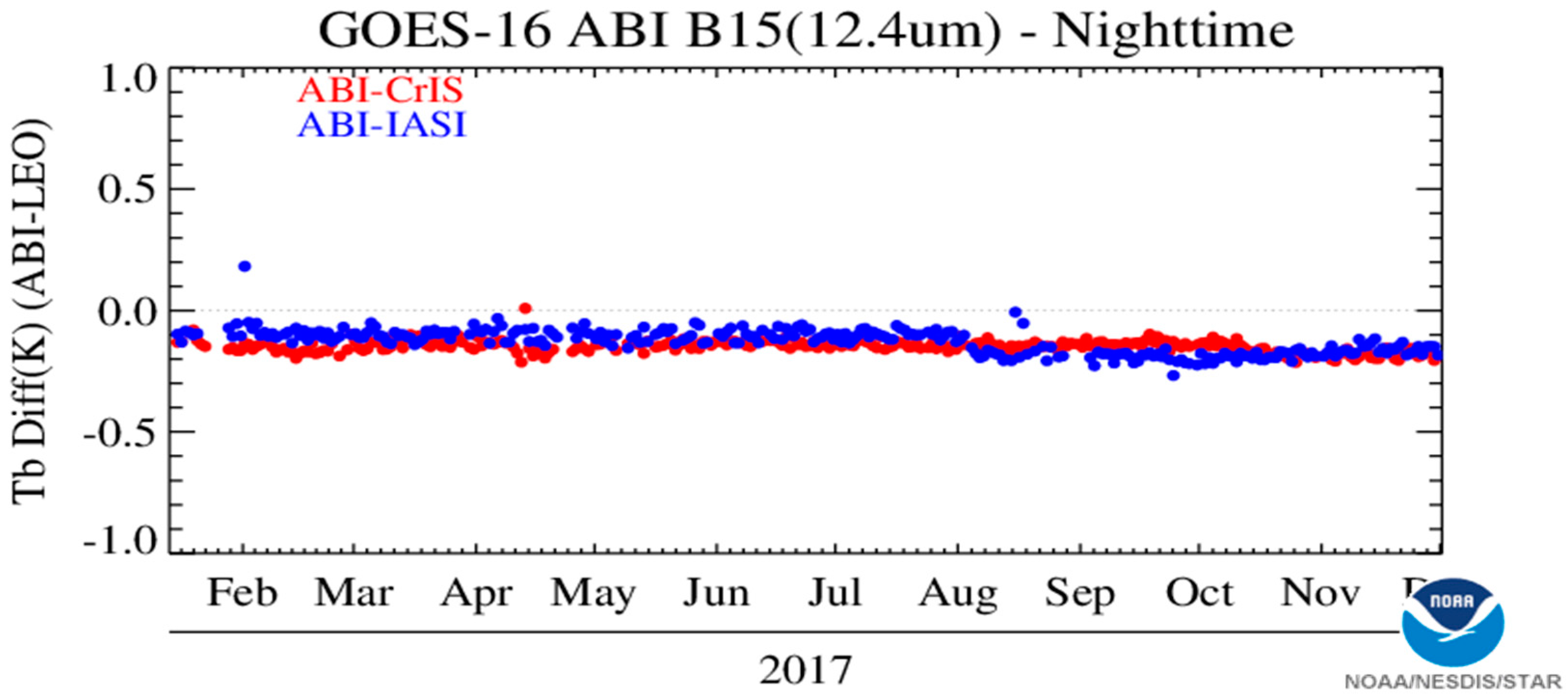
4.1. Radiometric Performance

ABI Calibration performance is constantly monitored by scientists of GOES-R CWG to detect deficiency, investigate root cause, propose improvement, verify update, and document the events to inform users, operator, vendor, and managers [16]. Figure 15 shows the time series of signal to noise ratio (SNR) for GOES-16 ABI visible and near infrared (VNIR) channels since launch. The minimum specified SNR requirements for resampled pixels is 300. The plotted values are the mean and standard deviation of SNR’s for individual detectors, derived from SCT measurements and converted to pixel SNR with resampler noise reduction factor. A higher than the required SNR indicates that the sensor is performing better than the design specifications.

Figure 16 is an example of ABI calibration performance verification, where ABI IR radiances in band 15 are compared with the radiances of two hyperspectral instruments, the Cross-track Infrared Sounder (CrIS) and the Infrared Atmospheric Sounding Interferometer (IASI). With few exceptions, the differences between ABI and hyperspectral instruments are small and steady over time. The small change of ABI-IASI comparison in early August was due to a change in IASI calibration algorithm; note the absence of ABI-CrIS comparison at the same time. An even smaller change in middle October, where there are minor ABI-CrIS and ABI-IASI differences (i.e., the red and blue dots are closer to be on top of each other), was due to an update of ABI scan mirror emissivity. The ability of detecting differences of such small magnitude, as well as the changes of differences in time, lends confidence in the evaluation of ABI performance.

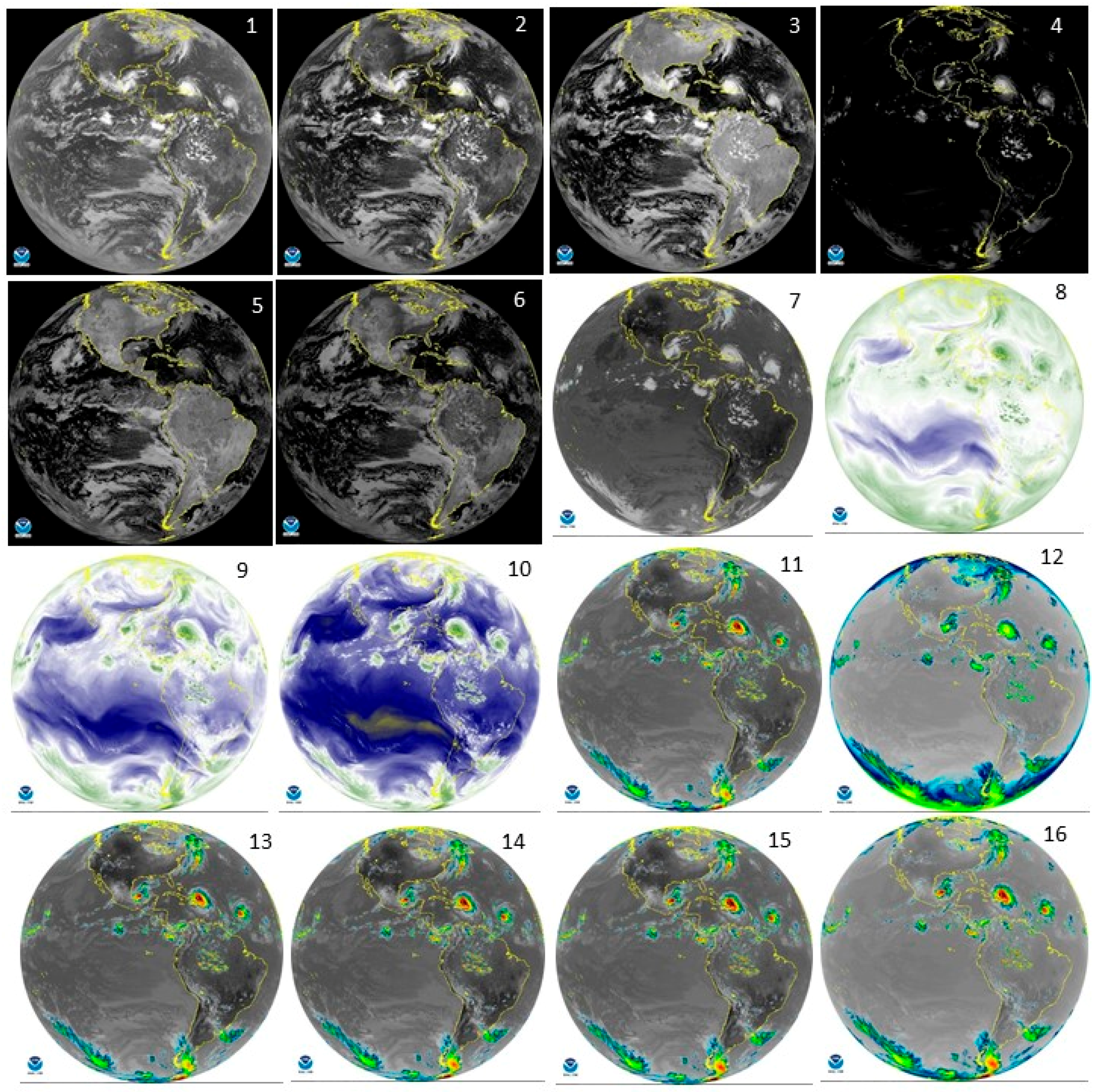
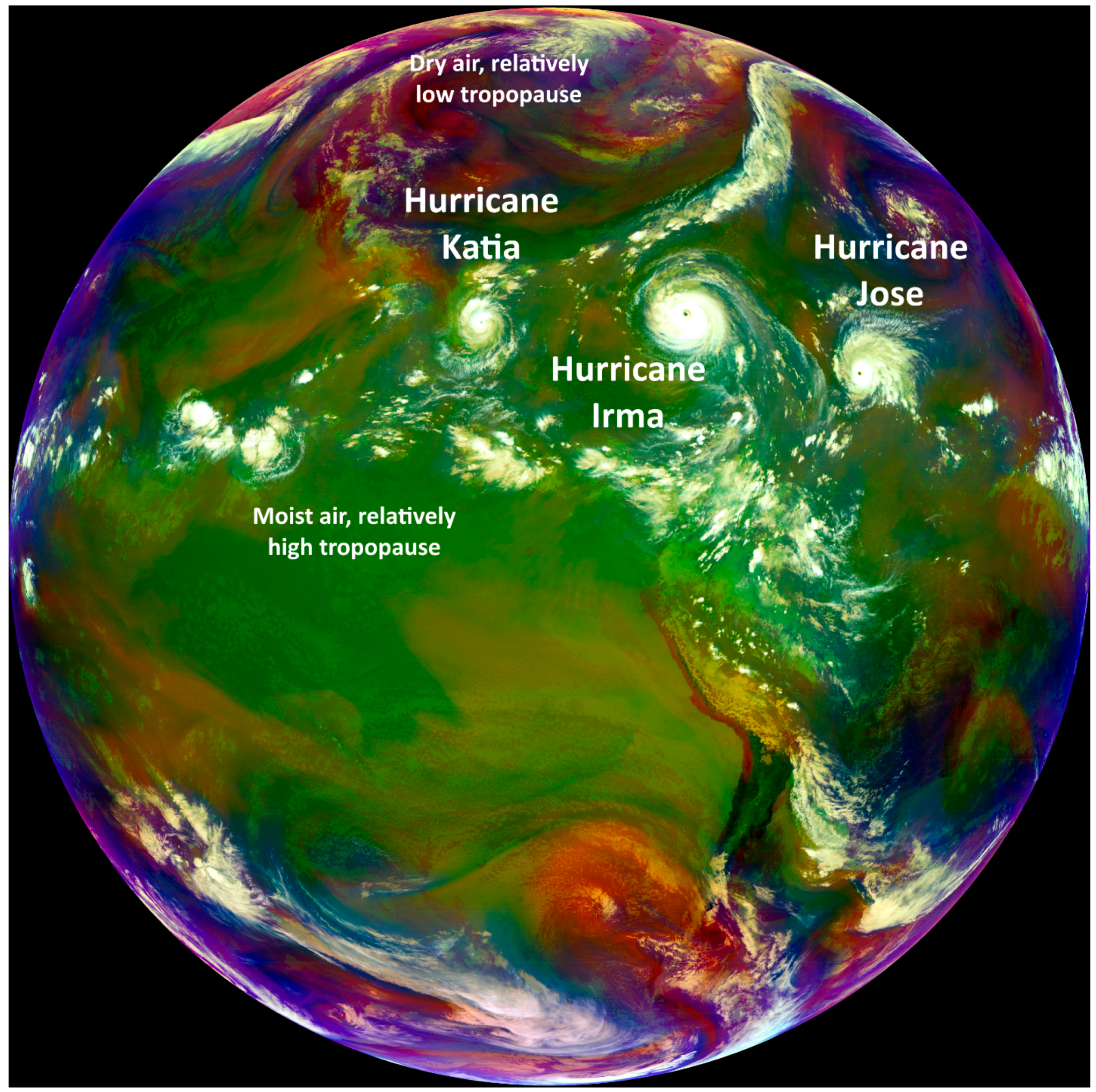
4.2. Improved Spectral Resolution

ABI has 16 spectral bands (Figure 17), compared to only 5 with the legacy GOES Imager. This is a significant upgrade to legacy GOES Imagers and allows the generation of some products that were previously possible only from polar-orbiting instruments, such as the Moderate Resolution Imaging Spectroradiometer (MODIS) or the Visible Infrared Imaging Radiometer Suite (VIIRS). This improved capability allows the detection and monitoring of a wide variety of Earth science applications and phenomenon in greater detail and accuracy. For example, Figure 18 shows how different spectral bands from ABI are combined to create a Red-Green-Blue (RGB) false color “Air Mass” image designed and tuned for monitoring the evolution of cyclones, in particular, rapid cyclogenesis, jet streaks, and Potential Vorticity (PV) anomalies as well as detection of volcanic SO₂ plumes [17,18,19,20]. The red component is the difference between the 6.2 (ABI band 8) and 7.3 (band 10) µm water vapor bands, green is the 9.6 µm ozone absorption (band 12) minus the window IR 10.3 µm band (band 13), and blue is the 6.2 µm band (band 8) alone. The resulting image allows forecasters to easily identify the general air mass classification based on color. Variations in red are indicative of variations in vertical temperature and water vapor profiles in the atmosphere; dry atmosphere has lower temperature differences between bands 8 and 10 and appears brighter red than moist areas. Shades of green indicate variation in ozone, which is directly related to stratospheric air temperature; polar air masses with lower tropopause heights are rich in column Ozone, and thus have larger temperature differences than warm tropical air. Blue indicates upper level tropospheric water vapor in the atmosphere, and is used for tracking jet streams and hurricanes; warm air masses at the edge of the Earth (limb) appear dark blue when viewed at large view angles (limb-cooling).

4.3. Improved Spatial Resolution

ABI spatial resolution improved from the legacy GOES imager in both the visible (0.5 km nadir spatial resolution in band 2 (Table 1) v/s 1.0 km nadir resolution in GOES-I-M band 1) and infrared (2 km v/s 4 km). Figure 19 shows a comparison of the eye of Hurricane Harvey from 25 August 2017 as viewed from the GOES-16 ABI visible band 2 (Figure 19a) and the GOES-13 visible band 1 (Figure 19b). The map line of the Texas coast can be seen in the northwest corner of the images; at this time the storm was still over the Gulf of Mexico. Improved clarity of the ABI image is evident, as the GOES-13 visible imagery is significantly blurrier. Details of the low-level clouds within the hurricane’s eye, as well as textured cloud tops in the eyewall region are both improved with the ABI.

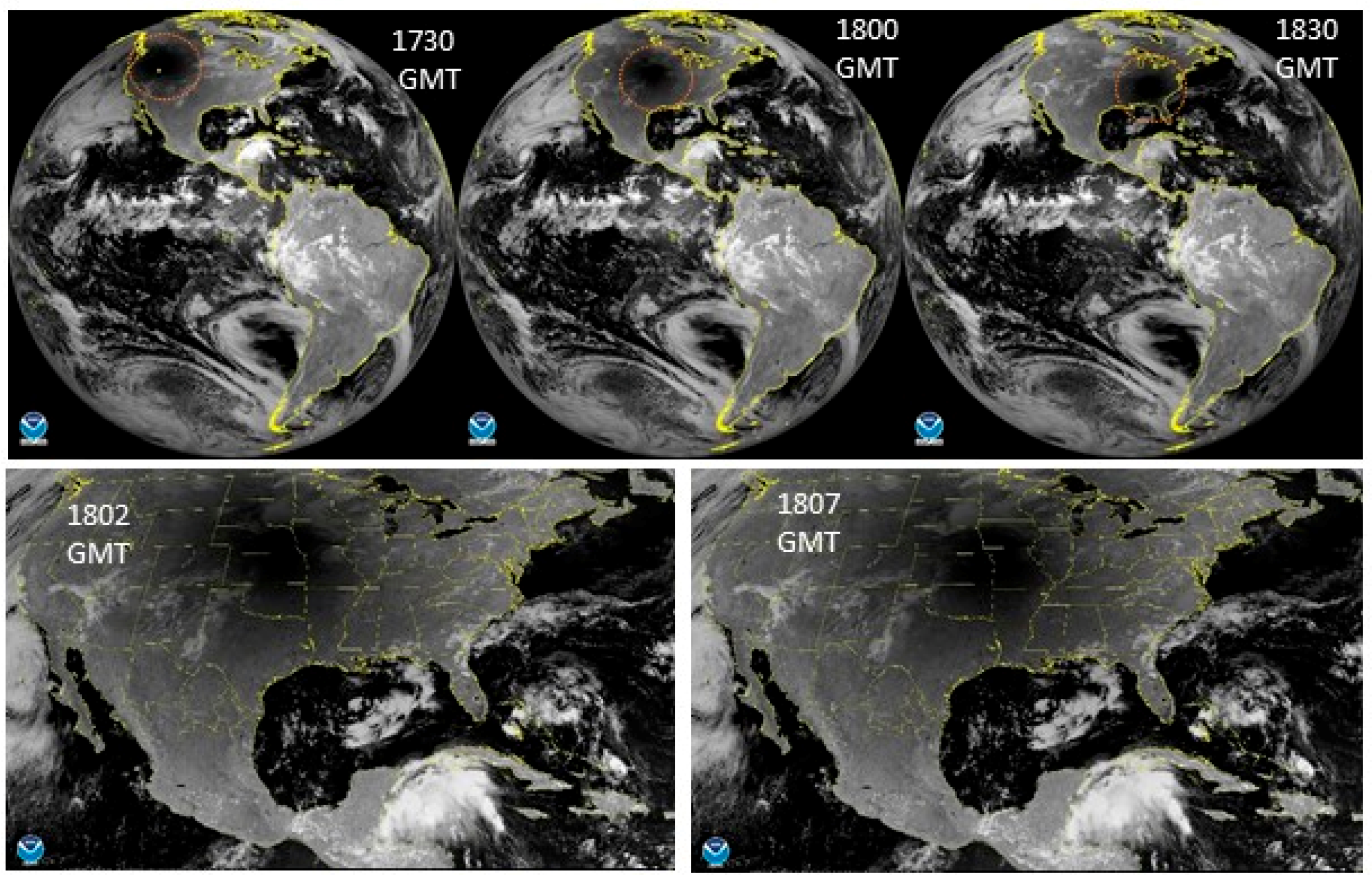
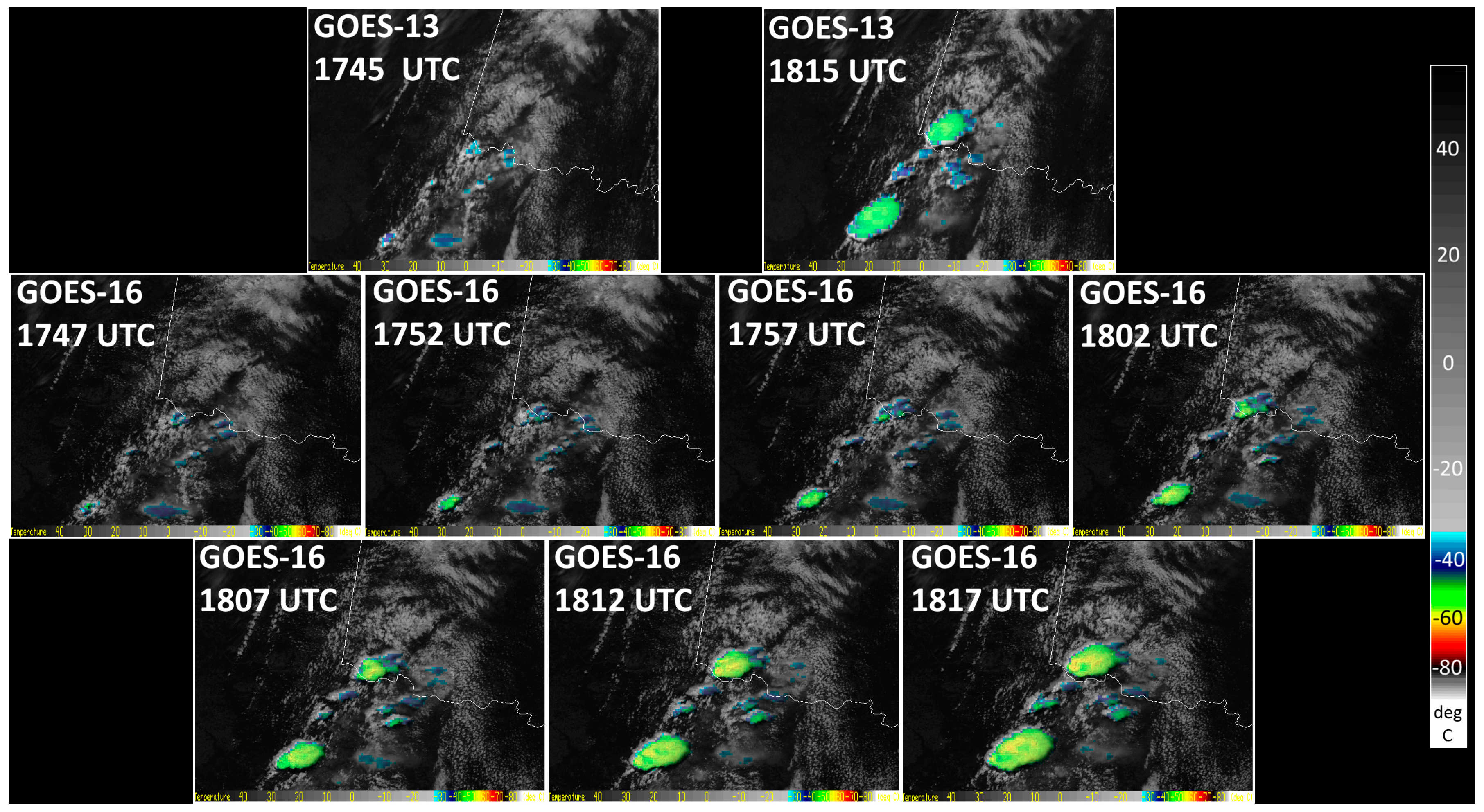
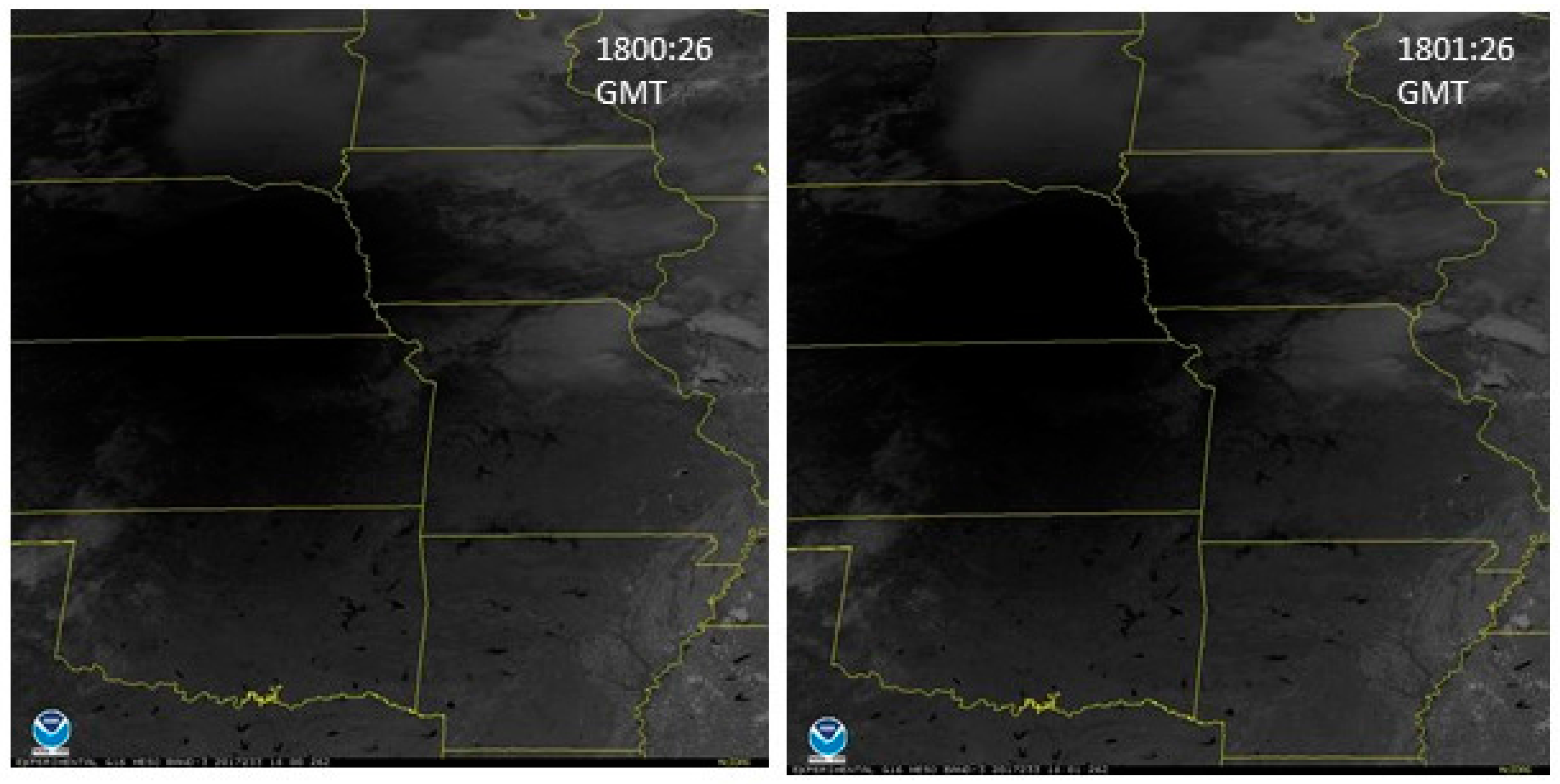
4.4. Improved Temporal Resolution

Earlier experiments with the GOES-14 legacy imager collected in the Super Rapid Scan Operations (SRSOR) demonstrated the utility and uniqueness of one-minute imagery in providing insights into the meteorological processes before, during and after severe weather events [21,22], albeit at the lower 1-km spatial resolution compared to the 0.5-km resolution of ABI. The flexibility of ABI to collect imagery more rapidly and at higher spatial resolution compared to the legacy GOES imagers offers unique opportunities to detect and monitor rapidly evolving meteorological phenomenon such as convective storms and hurricanes much more effectively than before across the entire hemisphere. For example, Figure 20 shows rapid Convective Initiation (CI) over a region covering Texas and Oklahoma on 18 May 2017 as observed by the legacy GOES-13 Imager (top panel) and ABI (middle and bottom panels). Between 1745 and 1815 GMT only two images were collected by the GOES-13 imager since full disk images can only be collected at least 30 min apart by the legacy sensor. As a result, GOES-13 missed the rapid development of the convective clouds completely.

The images in the middle and bottom panels are from ABI on GOES-16 showing successive 5-min CONUS scans. This improved temporal sampling allowed a closer look at the formation of the storms. It should also be noted that GOES-16 1-min mesoscale sector imagery was also available over this domain, providing 5 times more images than are shown in Figure 20.

During the early checkout and commissioning phase of ABI on GOES-16, the total solar eclipse over the US on 21 August 2017 offered a unique opportunity to image the rapidly moving shadow of the moon over the Earth during the eclipse at multiple temporal frequencies in all spectral bands concurrently to demonstrate this capability. Figure 21 shows the moon’s shadow during the eclipse collected in band 3 (0.86 µm) concurrently every 15 min over the full disk, 5 min over the CONUS and 1 min over a mesoscale sector by ABI in Mode 3. At the time of writing this manuscript, ABI imagery collected in Mode 3 was successfully used by forecasters to track several major Atlantic hurricanes such as Harvey, Irma, Jose and Katia (Figure 18).

5. Summary

ABI has significant technical enhancements over the legacy GOES imager that allow collection of Earth observations at improved spectral, spatial and temporal resolution as well as advanced capabilities for calibration and navigation. New and improved algorithms have been developed and implemented in the GOES-R ground system to process raw observations from ABI into calibrated and geolocated imagery to take advantage of full capabilities of the sensor. Early results from the mission demonstrate that ABI is performing as designed, the ground processing algorithms are processing the raw data into imagery that is of superior quality than legacy GOES imager. ABI is already having a significant impact on meteorologists ability to monitor and track significant meteorological events in greater detail than before. When GOES-S satellite is launched in 2018 and moved into operations, ABI from both GOES East and West will provide unprecedented coverage of the entire Western Hemisphere.

References

1. Kalluri, S.; Gundy, J.; Haman, B.; Paullin, A.; Van Rompay, P.; Vititoe, D.; Weiner, A.A. High Performance Remote Sensing Product Generation System Based on a Service Oriented Architecture for the Next Generation of Geostationary Operational Environmental Satellites. Remote Sens. 2015, 7, 10385–10399. [Google Scholar] [CrossRef]
2. Schmit, T.J.; Gunshor, M.M.; Menzel, W.P.; Gurka, J.J.; Li, J.; Bachmeier, A.S. Introducing the next generation Advanced Baseline Imager on GOES-R. Bull. Am. Meteorol. Soc. 2005, 86, 1079–1096. [Google Scholar] [CrossRef]
3. Schmit, T.J.; Griffith, P.; Gunshor, M.M.; Daniels, J.M.; Goodman, S.J.; Lebair, W.J. A Closer Look at the ABI on the GOES-R Series. Bull. Am. Meteorol. Soc. 2017, 98, 681–698. [Google Scholar] [CrossRef]
4. Kieffer, H.H.; Stone, T.C. The spectral irradiance of the Moon. Astron. J. 2005, 129, 2887–2901. [Google Scholar] [CrossRef]
5. Goldberg, M.; Ohring, G.; Butler, J.; Cao, C.; Datla, R.; Doelling, D.; Gärtner, V.; Hewison, T.; Iacovazzi, B.; Kim, D.; et al. The Global Space-Based Inter-Calibration System. Bull. Am. Meteorol. Soc. 2011, 92, 467–475. [Google Scholar] [CrossRef]
6. Consultative Committee for Space Data Systems (CCSDS) Blue Books: Recommended Standards. Available online: http://ccsds.cosmos.ru/publications/BlueBooks.aspx (accessed on 25 January 2018).
7. Datla, R.; Shao, X.; Cao, C.; Wu, X. Comparison of the Calibration Algorithms and SI Traceability of MODIS, VIIRS, GOES, and GOES-R ABI Sensors. Remote Sens. 2016, 8, 126. [Google Scholar] [CrossRef]
8. Griffith, P.C. 11.2 ABI’s Unique Calibration and Validation Capabilities. In Proceedings of the 12th Annual Symposium on New Generation Operational Environmental Satellite Systems, AMS Annual Meeting, New Orleans, LA, USA, 11–14 January 2016. [Google Scholar]
9. Okuyama, A.; Andou, A.; Date, K.; Hoasaka, K.; Mori, N.; Murata, H.; Tabata, T.; Takahashi, M.; Yoshino, R.; Bessho, K. Preliminary validation of Himawari-8/AHI navigation and calibration. Proc. SPIE 2015, 9607, 96072E. [Google Scholar]
10. GOES-R Product Definition and Users’ Guide (PUG) Volume 3 (L1b Products), Revision F. 2017. Available online: http://www.goes-r.gov/users/docs/PUG-L1b-vol3.pdf (accessed on 25 January 2018).
11. Gibbs, B.P.; Carr, J.L. GOES-R Orbit and Instrument Attitude Determination. In Proceedings of the 24th International Symposium on Space Flight Dynamics, Columbia, MD, USA, 5–9 May 2014. [Google Scholar]
12. GOES-R General Interface Requirements Document (GIRD) 417-R-GIRD-0009, Version 2.24, NASA GSFC. 2004. Available online: http://www.goes-r.gov/syseng/docs/GIRD_V_2_24.pdf (accessed on 25 January 2018).
13. Igli, D.; Virgilio, V.; Grounder, K. Image navigation and registration for GOES-R advanced baseline imager. In Proceedings of the 2009 AAS Guidance and Control Conference, Breckenridge, CO, USA, 30 January–4 February 2009. [Google Scholar]
14. Chapel, J.; Stancliffe, D.; Bevacqua, T.; Winkler, S.; Clapp, B.; Rood, T.; Gaylor, D.; Freesland, D.; Krimchansky, A. Guidance, navigation, and control performance for the GOES-R spacecraft. CEAS Space J. 2015, 7, 87–104. [Google Scholar] [CrossRef]
15. Shuttle Radar Topography Mission. Available online: https://www2.jpl.nasa.gov/srtm/ (accessed on 25 January 2018).
16. Yu, F.; Wu, X.; Shao, X.; Efremova, B.V.; Yoo, H.; Qian, H.; Iacovazzi, R.A. Early radiometric calibration performances of GOES-16 Advanced Baseline Imager (ABI). Proc. SPIE 2017, 10402, 104020S. [Google Scholar]
17. Santurette, E.P.; Georgiev, C.G. Weather Analysis and Forecasting: Applying Satellite Water Vapor Imagery and Potential Vorticity Analysis; Elsevier: Amsterdam, The Netherlands; Academic Press: Cambridge, MA, USA, 2005. [Google Scholar]
18. Tjemkes, S.; Duff, C.; Elliott, S. Total Ozone from Meteosat Second Generation. In Proceedings of the Meteorological Satellite Data Users’ Conference, Weimar, Germany, 29 September–3 October 2003; pp. 306–311. [Google Scholar]
19. Rosting, B.; Sunde, J. Application of Meteosat WV images in monitoring of synoptic scale cyclogenesis. In Proceedings of the Meteorological Satellite Data Users’ Conference, Vienna, Austria, 16–20 September 1996; pp. 119–126. [Google Scholar]
20. Bader, M.J.; Grant, J.R.; Waters, A.J.; Forbes, G.J. Images in Weather Forecasting: A Practical Guide for Interpreting Satellite and Radar Imagery; Cambridge University Press: New York, NY, USA, 1995. [Google Scholar]
21. Line, W.E.; Schmit, T.J.; Lindsey, D.T.; Goodman, S.J. Use of Geostationary Super Rapid Scan Satellite Imagery by the Storm Prediction Center. Weather Forecast. 2016, 31, 483–494. [Google Scholar] [CrossRef]
22. Schmit, T.J.; Goodman, S.J.; Lindsey, D.T.; Rabin, R.M.; Bedka, K.M.; Gunshor, M.M.; Cintineo, J.L.; Velden, C.S.; Bachmeier, A.S.; Lindstrom, S.S.; et al. Geostationary Operational Environmental Satellite (GOES)-14 super rapid scan operations to prepare for GOES-R. J. Appl. Remote Sens. 2013, 7, 073462. [Google Scholar] [CrossRef]
23. Setvak, M.; Lindsey, D.T.; Novak, P.; Wang, P.K.; Radova, M.; Kerkmann, J.; Grasso, L.; Su, S.; Rabin, R.M.; Stastka, J.; et al. Satellite-observed cold-ring-shaped features atop deep convective clouds. Atmos. Res. 2010, 97, 80–96. [Google Scholar] [CrossRef]
Figure 1. The Advanced Baseline Imager.
Remotesensing 10 00177 g001
Figure 2. ABI optical components. (SM = Scan Mirror; EW = East–West; NS = North–South; FMA = Four Mirror Anastigmat; S1, S2 = Beamsplitter 1 and 2; CS = Cold Stop; W1, W2, W3 = Windows 1, 2, and 3; LWIR = Longwave Infrared; VNIR = Visible and Near IR; MW IR = Mid-Wave IR).
Remotesensing 10 00177 g002
Figure 3. Graphic representation of mirrors and a detector array for the 1.61 µm spectral band (6 columns and 676 rows). Within each focal plane array, there are multiple detector elements in each row, the best of which is selected for output on a row-by-row basis. Each “Frame” is the output of one integration time. Operating the scan mirror 1 (North–South) and scan mirror 2 (East–West) together results in 22 swaths that cover the entire observable hemisphere.
Remotesensing 10 00177 g003
Figure 4. Scanning pattern of the legacy GOES Imagers (left) vs the ABI scanning pattern (right).
Remotesensing 10 00177 g004
Figure 5. Noise Equivalent change in radiances expressed in units of temperature at 300 K for the legacy Imagers on GOES 12, 15, and ABI on GOES-16. The ABI sensor requirements are NEdT of up to 0.1 K for bands 7–15 and a NEdT of up to 0.3 K for band 16. The central wave lengths of legacy GOES Imager IR bands shown here are close to ABI but not identical (data from the Calibration Working Group, NOAA/NESDIS/STAR).
Remotesensing 10 00177 g005
Figure 6. An ABI image of the Moon and portion of the Earth observed by GOES-16 on 11 January 2017 in band 2 (0.64 µm).
Remotesensing 10 00177 g006
Figure 7. Graphic representation of the Level 0 data structure for ABI.
Remotesensing 10 00177 g007
Figure 8. Graphic representation of the Level 1a data structure for ABI.
Remotesensing 10 00177 g008
Figure 9. The same fixed-grid coordinates map to the same latitude and longitude for all ABI L1 and L2 products in accordance with the algorithm defined in the PUG [10]. The relationship between the fixed-grid and geographic coordinates depends on the reference longitude. The purple circle shows the sub-satellite point on the hemisphere, and the red cross shows the center of the CONUS area.
Remotesensing 10 00177 g009
Figure 10. East to West and North to South observation geometry of the Earth about the satellite’s x and y axis, respectively (A). The 0.5-km, 1-km, and 2-km spatial resolution map grids are exactly registered to each other (B,C).
Remotesensing 10 00177 g010
Figure 11. Fixed-grid coordinates are defined by an idealized scanning system where the NS angle elevates the EW-scan plane with respect to the equator [11]. This definition follows that of the legacy GOES-NOP system, but other operators such as EUMETSAT and JMA use a convention where the order of rotations is swapped.
Remotesensing 10 00177 g011
Figure 12. INR processing is implemented on the ground and relies on star scans, attitude rates, scan mirror angular encoder readouts, and an orbit determined from onboard GPS. A Kalman Filter with delayed state update smoothing navigates the VNIR channels, and a separate sliding window batch estimator fits the alignment between the VNIR and IR channels.
Remotesensing 10 00177 g012
Figure 13. The value for each pixel p is calculated as a weighted average of neighboring detector samples with resampling weights drawn from a resampling kernel function.
Remotesensing 10 00177 g013
Figure 14. Navigation (NAV) and Frame-to-Frame Registration (FFR) performance metrics for band 2 full disk scenes demonstrate compliance with respect to their respective INR specifications. The metric is calculated as the absolute value of the mean error plus three times the standard deviation computed over a 24-h sliding window. Mean NAV and FFR errors are also aggregated by scene and plotted here.
Remotesensing 10 00177 g014
Figure 15. Time series of signal to noise ratio (SNR) for GOES-16 ABI visible and near infrared (VNIR) channels since launch (data from the Calibration Working Group, NOAA/NESDIS/STAR).
Remotesensing 10 00177 g015
Figure 16. Difference of radiance, expressed in terms of brightness temperature (Tb in K), plotted as a function of time since the ABI data were received in January 2017. The red and blue dots are ABI differences from CrIS and IASI, respectively.
Remotesensing 10 00177 g016
Figure 17. ABI full disk images of all 16 bands collected on 7 September 2017 at 1830 UTC. The band numbers are indicated on the top right of each image.
Remotesensing 10 00177 g017
Figure 18. Airmass RGB from GOES-16 from 8 September 2017 at 1745 UTC. This product is created by applying 6.2–7.3 µm, 9.6–10.3 µm, and 6.2 µm band differences/bands to the red, green, and blue components, respectively.
Remotesensing 10 00177 g018
Figure 19. A comparison of the eye of Hurricane Harvey from 25 August 2017 at 2015 UTC as it approached the Texas coast from: (a) GOES-16 band 2; and (b) GOES-13 band 1.
Remotesensing 10 00177 g019
Figure 20. Top panels show images collected by GOES-13 Imager, and the middle and bottom panels show images collected by ABI on GOES-16. The geographic area covering parts of Texas and Oklahoma were extracted from the GOES-13 full disk imagery that is collected every 30 min. ABI collected data every 5 min over the same region. Both GOES-13 and GOES-16 images shown here are created using similar visible (band 1 from Imager and band 2 from ABI) and IR bands (band 4 from Imager and band 13 for ABI) [23]. The IR data have been color enhanced based on brightness temperature (in °C) and made partially transparent so that information from the visible can also be seen.
Remotesensing 10 00177 g020
Figure 21. ABI images collected in band 3 (0.86 µm) on 21 August 2017, the day of total solar eclipse over United States. Top panel shows ABI full disk images collected at 1730Z, 1800Z and 1830Z (full disk data are collected every 15 min in Mode 3, but only alternate scenes are shown here). The outlined dark spot shows the shadow of the solar eclipse on the Earth. The middle and lower panels show the CONUS (every 5 min) and mesoscale imagery (every 1 min) respectively. Observation times are shown on the top right of each image.
Remotesensing 10 00177 g021aRemotesensing 10 00177 g021b