Abstract
As the global population increases, we face increasing demand for food and nutrition. Remote sensing can help monitor food availability to assess global food security rapidly and accurately enough to inform decision-making. However, advances in remote sensing technology are still often limited to multispectral broadband sensors. Although these sensors have many applications, they can be limited in studying agricultural crop characteristics such as differentiating crop types and their growth stages with a high degree of accuracy and detail. In contrast, hyperspectral data contain continuous narrowbands that provide data in terms of spectral signatures rather than a few data points along the spectrum, and hence can help advance the study of crop characteristics. To better understand and advance this idea, we conducted a detailed study of five leading world crops (corn, soybean, winter wheat, rice, and cotton) that occupy 75% and 54% of principal crop areas in the United States and the world respectively. The study was conducted in seven agroecological zones of the United States using 99 Earth Observing-1 (EO-1) Hyperion hyperspectral images from 2008–2015 at 30 m resolution. The authors first developed a first-of-its-kind comprehensive Hyperion-derived Hyperspectral Imaging Spectral Library of Agricultural crops (HISA) of these crops in the US based on USDA Cropland Data Layer (CDL) reference data. Principal Component Analysis was used to eliminate redundant bands by using factor loadings to determine which bands most influenced the first few principal components. This resulted in the establishment of 30 optimal hyperspectral narrowbands (OHNBs) for the study of agricultural crops. The rest of the 242 Hyperion HNBs were redundant, uncalibrated, or noisy. Crop types and crop growth stages were classified using linear discriminant analysis (LDA) and support vector machines (SVM) in the Google Earth Engine cloud computing platform using the 30 optimal HNBs (OHNBs). The best overall accuracies were between 75% to 95% in classifying crop types and their growth stages, which were achieved using 15–20 HNBs in the majority of cases. However, in complex cases (e.g., 4 or more crops in a Hyperion image) 25–30 HNBs were required to achieve optimal accuracies. Beyond 25–30 bands, accuracies asymptote. This research makes a significant contribution towards understanding modeling, mapping, and monitoring agricultural crops using data from upcoming hyperspectral satellites, such as NASA’s Surface Biology and Geology mission (formerly HyspIRI mission) and the recently launched HysIS (Indian Hyperspectral Imaging Satellite, 55 bands over 400–950 nm in VNIR and 165 bands over 900–2500 nm in SWIR), and contributions in advancing the building of a novel, first-of-its-kind global hyperspectral imaging spectral-library of agricultural crops (GHISA: www.usgs.gov/WGSC/GHISA).
1. Introduction
Increasing global populations, trends toward urbanization, and changes in dietary preferences necessitate rapid monitoring of global agricultural croplands and their characteristics [1]. Remote sensing has made such monitoring possible, and advances in remote sensing technology facilitate global assessment. For example, WorldView-4, launched on 11 November 2016, has a spatial resolution of 1.24 m (0.30 m in the panchromatic band), with four multispectral bands in the visible and near infrared regions. Additionally, the combined use of Landsat and Sentinel imagery allows for an increase in temporal resolution. Recently, there have also been advances in spectral resolutions of multispectral sensors, including WorldView-3 [2] and Sentinel-2 [3]. However, hyperspectral data take it to the next level where spectral data points are replaced by spectral signatures, as demonstrated in several vegetation studies [4,5,6]. Even high spatial resolution multispectral data underperform when compared with hyperspectral data [7,8]. This is because multispectral data are limited in two ways. Firstly, they have few broad bands over a wide spectral range that lead to gaps in spectral coverage. Secondly, these bands average spectral information over a large spectral region, masking narrow spectral features.
In contrast, hyperspectral sensors have 100s to 1000s of narrow wavebands providing continuous coverage across the spectral profile. Such hyperspectral data have been used for many applications, including invasive species control [9,10,11], biodiversity estimation [12], vegetation/land cover/crop residue classification [13,14,15,16,17,18,19,20], biochemical characteristics modeling [21], pollution assessment [22,23,24], and various agricultural applications [25,26,27].
Although recently decommissioned, the hyperspectral Hyperion satellite provided data at a spatial resolution of 30 m and spectral resolution of 242 bands (220 of which are unique and radiometrically calibrated) globally from 2001 to 2016. Over 70,000 Hyperion images are freely available through the USGS EarthExplorer and have been used for several applications including classification of land cover classes [28,29,30], alteration minerals [31], rocks and land formations [32], plant and tree species [29,33,34,35,36,37] including invasive species [38,39], and vegetation functional types [40]. Additionally, these data have been used to monitor mine waste [41], estimate foliar nutrition [42] and photosynthetic activity [43], and assess fire danger and post-fire effects [44,45]. Agricultural studies using Hyperion data include classification of crop residue [46,47], crops and crop varieties [48,49], crop planting area [50], and crop conditions after harvest [51]. These data have also been used to assess tillage intensity [47], and crop biophysical and biochemical characteristics [8,52,53,54,55]. Nevertheless, these studies almost always use one or a few Hyperion images at most, with each Hyperion image being 7.5 km by 100 km. In contrast, in this research we implement a comprehensive, country-wide assessment of Hyperion images in different agroecological zones (AEZs) of the US.
Hyperspectral narrowbands have out-performed multispectral broadbands in crop productivity estimation [55], crop type discrimination [8], and biomass variability assessment [29]. However, these large datasets can be challenging to preprocess, process, and analyze. These challenges are ameliorated through the use of machine learning and cloud computing. The Google Earth Engine (GEE) cloud computing platform [56], which has already ingested most Hyperion images, in WGS84 projection, allows a user to work with hundreds of Hyperion images without having to download them on a personal computer. The image collection can quickly be filtered and processed using Google’s processing power. Codes can quickly be shared for debugging and collaboration.
Thus, the overarching goal of this research was to use 30 m EO-1 Hyperion hyperspectral data in a comprehensive study of agricultural crops, specifically classifying and separating crop types and crop growth stages of five leading world crops (corn, soybean, winter wheat, rice, and cotton) that occupy approximately 75% of the US principal cropland area and 54% of the world’s principal cropland area (Table 1). Specific objectives of the research were to:

Table 1.
Principal crops of the world. Five leading world crops that also occupy an overwhelming proportion of the principal cropland areas of the US (Sources: US data from [62], area planted in 2017. World data derived from [54], area harvested in 2000).
- Develop a Hyperspectral Imaging Spectral library of Agricultural crops (HISA), of five principal crops of the US, using Hyperion satellite data.
- Establish optimal hyperspectral narrowbands (OHNBs) of Hyperion to study agricultural crops in the US and to overcome data redundancy.
- Classify the five leading principal crops in the US using multiple Hyperion images from distinct AEZs to determine the strengths and limitations of OHNBs in classifying crop types and crop growth stages.
- Demonstrate the power of computing large volumes of Hyperion data on the GEE cloud computing platform. Although much research has been done on determining best bands for studying crops, this study contributes unique knowledge due to its use of 99 Hyperion images throughout different AEZs in the US to study five globally dominant crops. The results from this research will help us prepare for processing large datasets that will be generated by upcoming hyperspectral satellites like EnMAP and the Surface Biology and Geology mission (formerly HyspIRI mission) [57], as well as the DLR Earth Sensing Imaging Spectrometer (DESIS) which is already on the ISS-MUSES platform [58], and automating that processing in a cloud-computing platform. This will enable us to study and characterize agricultural crops and advance their modeling and mapping, which in turn will help in advancing food security analysis.
2. Materials and Methodology
2.1. Study Area
We focused on the US in this study because of the availability of the high quality training and validation data from the US Department of Agriculture Cropland Data Layer (CDL), a wall-to-wall high spatial resolution dataset on crop type and location. This dataset was used as a reference while compiling HISA. We selected 7 study areas in 7 AEZs (Figure 1) based on crop distribution, and the availability of cloud-free time series Hyperion images during the growing season. We used AEZs as defined by the Food and Agriculture Organization (FAO) [59], and selected one study area in each of 7 AEZs.
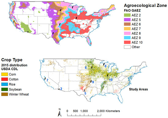
Figure 1.
Study areas throughout the US in various agroecological zones (AEZs). US study areas, named according to AEZs in which they are located. AEZs as defined by Food and Agriculture Organization (FAO) [59].
2.2. Datasets
2.2.1. Reference Data of Agricultural Crops in the US
The USDA CDL dataset [60] is available for the entire US from 2008 to present, from which reference training and validation data were gathered. We focused on five principal crops (corn, cotton, rice, soybean, and winter wheat) because these are the dominant crops within the US and the world (Table 1). The USDA CDL is the gold standard for crop maps, with wall-to-wall coverage of the US at high spatial resolutions with high classification accuracies (Table 2) [61]. Given these high accuracies, the USDA CDL is a highly reliable and respected reference data source.
Table 2.
Cropland Data Layer (CDL) Accuracies. USDA Cropland Data Layer accuracies for agroecological zones (AEZs), years, and crops of interest in this study.
Overall, we used a total of 99 Hyperion images (Table 3) spread across seven AEZs [59]. These images cover the five principal crops (Table 3) of the US.
Table 3.
Hyperion images in 7 AEZs and the leading world crops within these images. We used a total of 99 Hyperion hyperspectral images spread across 7 agroecological zones (AEZs) from 2008 to 2015 in the US. The dominant leading world crops in each of these images are also shown.
2.2.2. Preprocessing Hyperion Images: Steps Used in This Study
There are several steps recommended for preprocessing Hyperion data (Figure 2) [64]. We first separated the visible and near-infrared (VNIR) data from the shortwave infrared (SWIR) data because they are collected from two different spectrometers and have different calibration requirements. Then digital numbers (DNs, unitless) were converted to radiance (W m−2 sr−1 mm−1) by dividing VNIR DN by 40 and SWIR DN by 80, as described by several researchers including [65,66]. Atmospheric correction was done to convert radiance (W m−2 sr−1 mm−1) to surface reflectance (%). Problematic bands were then removed based on literature [29,55,67,68,69] and the authors’ observations of noisy bands. Bands at wavelengths from 427–925, 973–1104, 1165–1326, 1508–1770, and 2052–2355 nm were retained. All of these steps were coded and run in GEE, using the JavaScript API.
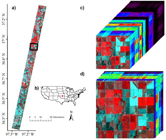
Figure 2.
Hyperion hyperspectral datacubes. (a) Earth Observing-1 (EO-1) Hyperion image over Ponca City, Oklahoma, USA, 2 September 2010, false color composite of RGB 844, 569, 529 nm; (b) locator map, with red rectangle showing location of Hyperion image; (c) datacube illustrating 198 bands available in Google Earth Engine (GEE) Hyperion data; (d) datacube illustrating 30 optimal hyperspectral narrowbands for studying globally dominant agricultural crops. Numerous band combinations are possible and important when using hyperspectral data. Here, we used 844 nm, 569 nm, and 529 nm. This is because, 844 nm is a center of NIR shoulder, 569 nm is at a point of steep slope within the green region, and 529 is at minimum slope, which allowed us to highlight the visual contrasts across different classes.
2.2.3. Atmospheric Correction of Hyperion Images
Atmospheric correction was done using the SMARTS model [70,71] and Equations (1)–(4) reported below. This model has been found to be 25 times faster than the 6S model, with only a 5% difference in results for satellite data processing [72]. Surface reflectance was calculated using Equation (1) [73], where L is at-satellite radiance in W m−2 sr−1 mm−1, is viewing angle in radians, E is solar irradiance in W m−2 sr−1 mm−1, is zenith angle in radians, T is transmittance (unitless) affected by various atmospheric elements, and E is diffuse downwelling radiance. Transmittance was calculated using Equation (2) [71], where T is Rayleigh transmittance (unitless) dependent on wavelength, , T is ozone transmittance (unitless), T is nitrogen dioxide transmittance (unitless), T uniformly mixed gas transmittance (unitless), T is water vapor transmittance (unitless), and T is aerosol transmittance (unitless). These transmittance components were calculated using equations described by [70,71]. E was calculated using Equation (3), where was calculated using Equation (4) [74]. Some of these equations require site-specific information, such as relative humidity, site-level pressure, and visibility. Visibility data were taken from the National Oceanic and Atmospheric Administration (NOAA) Integrated Surface Hourly (ISH) data [75]. Relative humidity and site-level pressure data were taken from University of Idaho’s Gridded Surface Meteorological (GRIDMET) dataset [76] and NASA’s North American Land Data Assimilation System 2 (NLDAS-2) data [75] respectively. GRIDMET and NLDAS-2 data are readily available in GEE.
2.2.4. Distribution of Data into Training and Validation Datasets
In total, 99 Hyperion images across seven AEZs in the US from 2008 to 2015 were selected based on image availability, crop distribution, and AEZ delineations (Figure 1, Table 3). Of the 99 Hyperion images, 11 images from 5 AEZs (Table 3) were used for crop type classifications and analysis because these images were acquired mostly during late vegetative or critical growth stages, when crops are best able to be classified. In AEZ 5, one image was used to differentiate cotton from winter wheat. In AEZs 6 and 10, three images each were used to differentiate corn from soybean. In AEZ 7, two images were used to differentiate corn from rice. Lastly, in AEZ 9, two images were used to differentiate corn, cotton, soybean, and winter wheat.
All 99 images across all seven AEZs were used for differentiating crop growth stages (Table 3). Out of these, 81 images in AEZs 6, 8, 9, and 10 were used to differentiate among corn growth stages (Table 3). Similarly, 56 images in AEZs 6, 9, and 10 were used to differentiate soybean growth stages. For cotton growth stage differentiation, 35 images in AEZs 2, 5, and 9 were used. For winter wheat, 31 images in AEZs 5 and 9 were used. Lastly, for rice, the 2 images from AEZ 7 were used.
Within the images, samples for data extraction were selected by overlaying Hyperion images on the USDA CDL in ArcMap and in GEE. Sufficiently rich and robust samples were selected for each crop, focusing on fields that had the same crop over multiple years. This enabled studies across years. Within those fields, a sample pixel was randomly selected, away from the edge to avoid edge effects. This was also done to take into account any issues in positional accuracy. The USDA CDL after 2005 inherits the positional accuracy of the image(s) used to derive the layer, including Landsat 4, 5, and 8, DEIMOS-1, DMC-UK 2, ESA Sentinel-2, and ISRO ResourceSat 2 LISS-3 [77]. When coordinates of specific features were compared between the CDL and Hyperion data, the difference was less than one pixel (i.e., <30 m). Once samples were selected, they were extracted from the surface reflectance image in GEE. Spectra were then smoothed in R using a moving average over 3 bands with the movav function in the Prospectr package [78], and compiled into a Hyperspectral Imaging Spectral library of Agricultural crops (HISA). There were three distinct Hyperion hyperspectral datasets that were obtained using the 99 images (Table 3). Within each dataset, 75% of samples were randomly selected in R for training, while the remaining 25% were used for validation. Classification accuracies achieved using linear discriminant analysis (LDA) and support vector machine (SVM) were all based on the independent validation samples. These validation samples were random, rich (collected across different AEZs for various crops throughout multiple years), and independent of training data. Since the samples were not used for training, they were ideal to validate the classification models. These datasets are discussed below.
Reference Training and Validation Datasets from Hyperion Images for Crop Type Linear Discriminant Analysis (LDA)
Crop type reference training and validation data (Table 4) were gathered from 11 images across 5 AEZs for the 5 crops using USDA CDL data for reference (Table 3). Overall, there were 2876 samples for training and 969 for validation. Across images, corn had 1104 training and 372 validation samples. Soybean had 1087 training and 366 validation samples. Winter wheat had 551 training and 184 validation samples. Rice had 86 training and 30 validation samples. Finally, cotton had 48 training and 17 validation samples. Illustrations of HISA for example Hyperion images, with spectral averages by crop type are included in Figure 3. These data were used for crop type separation using LDA.
Table 4.
Samples for crop type discrimination. Training and validation sample sizes for crop type discriminant analyses and image classification analyses; “other” only for image classification.
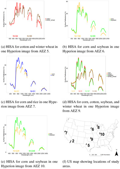
Figure 3.
Illustration of Hyperspectral Imaging Spectral library of Agricultural crops (HISA) of the US for 5 crops. HISA illustrated for 5 crops in certain agroecological zones and certain growth stages. N is number of spectra included in the average. HISA is part of the Global Hyperspectral Imaging Spectral-Library of Agricultural-crops (GHISA) (www.usgs.gov/WGSC/GHISA).
Reference Training and Validation Datasets from Hyperion Images for Crop Growth Stage Differentiation Using LDA
Crop growth stage reference training and validation data (Table 5) were gathered from 99 Hyperion images in seven AEZs (Table 3) for the 5 crops using USDA CDL data for reference. Overall, there were 5184 samples for training and 1739 for validation. Corn had 6 growth stages represented, with a total of 1916 training and 641 validation samples. Soybean had all 6 growth stages represented, and 1563 training and 523 validation samples. Winter wheat had 4 growth stages represented with 6188 training and 2076 validation samples. Cotton had 5 growth stages represented, with 615 training and 208 validation samples. Lastly, Rice had 2 of the 6 growth stages represented, with 86 training and 30 validation samples. An illustration of the Hyperion hyperspectral profiles averaged by crop growth stages is shown in Figure 4. These data were used for crop growth stage separation using LDA. A great strength of developing the global hyperspectral imaging spectral-library of agricultural-crops (GHISA) is shown in Figure 5. Late growth stage corn crop spectral signatures in AEZ10 during two years (2013 and 2014) with similar Julian Days show substantial spectral similarity. As a result of a 17-day difference in collection dates, we see some small differences in magnitude of the spectra at certain wavelengths. Corn spectra in the late growth stage from two different AEZs (AEZ10 and AEZ9) also show substantial similarities in the shape. However, since the two images were collected 26 days apart, we see differences in the magnitude of the spectral signatures, especially in the SWIR range. These results clearly demonstrate that it is possible to build a hyperspectral library of agricultural crops such as GHISA that has thousands of spectral signatures with such labels as “corn, late vegetative, irrigated, AEZ10”. These spectra can then be used to train models to classify satellite images in terms of crop types, their growth stages, their growing conditions, and a host of other factors (e.g., irrigation, N application, genome).
Table 5.
Training and validation samples for crop growth stage discrimination. Training and validation sample sizes for discriminant analyses across crop types in 7 agroecological zones (AEZs) using Hyperspectral Imaging Spectral library of Agricultural crops (HISA) of the US for each crop in each of the 6 growth stages, where present, derived from Hyperion data.
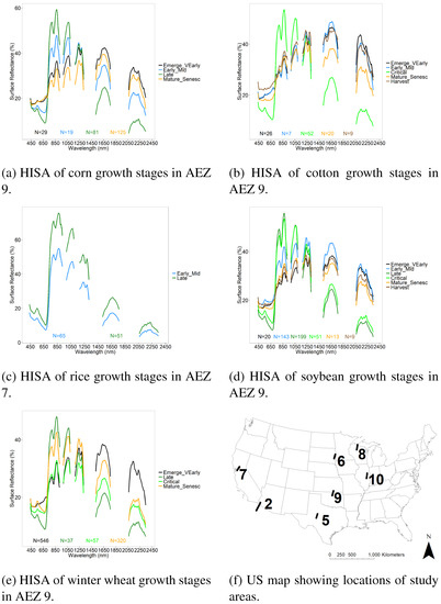
Figure 4.
Illustration of HISA of the US for 5 crops. Hyperspectral Imaging Spectral library of Agricultural crops (HISA) illustrated for 1 crop in 2 growth stages in AEZ 7, and 4–6 growth stages for the other crops in AEZ 9. N is number of spectra included in the average. HISA is part of the Global Hyperspectral Imaging Spectral-Library of Agricultural-crops (GHISA) (www.usgs.gov/WGSC/GHISA).
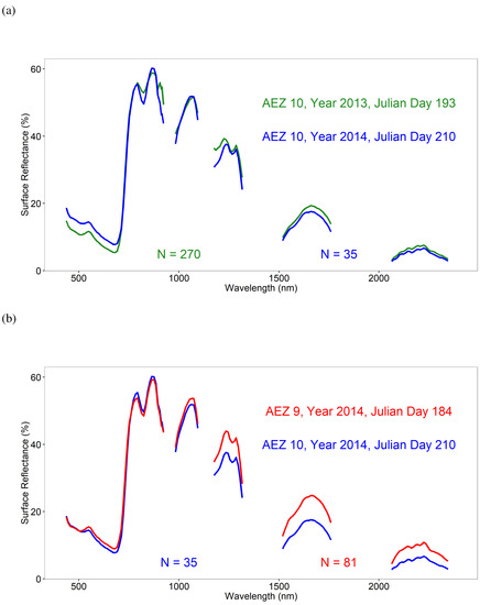
Figure 5.
Spectral matching of corn crop using EO-1 Hyperion data within and across agroecological zones (AEZs). Spectral matching of EO-1 Hyperion data taking corn crop spectra for the late growth stage: (a) within AEZ 10 for Julian Day 193 of year 2013 versus Julian Day 210 of year 2014; (b) across AEZs (AEZs 9 and 10) for Julian Day 210 of year 2014 in AEZ 10 versus Julian Day 184 of year 2014 in AEZ 9. N is number of samples used to calculate each average spectral profile.
Reference Training and Validation Datasets from Hyperion Images for Crop Type Image Classification and Mapping Using Support Vector Machines (SVM) in GEE
Crop type reference training and validation data (Table 4) were also gathered for 5 crops from the 11 images for Hyperion image classification using a pixel-based Support Vector Machines (SVMs) machine learning supervised classification algorithm run on the GEE cloud computing platform. Reference samples were collected from the same locations as those used for crop type discriminant analyses mentioned earlier, with the addition of an “other” class. This “other” class encompassed samples from non-croplands as well as crops other than the 5 included in this study. With this “other” class, there were 6439 training and 2159 validation samples. These spectra were extracted directly from the images and not smoothed. For each image, 75% of reference data were used for training the SVM, which was used to classify the entire image. The remaining 25% of data, not used in training, were used to assess classification accuracy.
2.3. Selection of OHNBs by Data Mining and Overcoming Data Redundancy
The best bands need to be selected to overcome data redundancy and autocorrelation, as well as issues related to the Hughes Phenomenon, which occurs because as the number of bands increases, the sample size also needs to increase to maintain statistical confidence in analyses [79]. Numerous dimensionality reduction methods and approaches were explored, including Principal Component Analysis (PCA, also used for data compression), Stepwise Discriminant Analysis (SDA), and Lambda-by-Lambda correlation plots [80,81] to name a few commonly used techniques. Several new techniques have recently been introduced to better handle non-linear [82] and dynamic [83] dimension reduction. It is clear from these studies that all methods have their strengths and limitations in agricultural studies [81]. We selected PCA because it is easy to implement, interpret, and understand, widely used [84], good with numerical variables [83], and successful at identifying the most important variables [85]. However, we encourage readers to explore multiple methods and approaches outlined in [80,81].
We conducted PCAs on spectra collected in late and critical growth stages of corn, cotton, rice, soybean, and winter wheat. Separate PCAs were run in R for the two growth stages and for the five crops. Enough principal components were retained to explain at least 98% of variability. Then, the ten most important bands were selected for each principal component based on factor loadings. Variables with the greatest absolute value of factor loadings are deemed most influential to a principal component. The overall 30 most important bands were then sequentially selected based on factor loadings, avoiding subsequent bands that were close to already-selected bands (Table 6).
Table 6.
Optimal Hyperion Hyperspectral Narrowbands (OHNBs) in agricultural studies. OHNBs based on Hyperion study of crops and growth stages, established by studying five leading agricultural crops in the US. Optimal bands found in this study are similar to those found to be important in studies by [54,79], thus re-affirming the importance of these non-redundant 30 OHNBs in studying agricultural crops. Feature descriptions adopted and modified from [79].
Out of these 30 bands, the most important 5, 10, 15, 20, 25, and 30 bands were selected (Table 7). These subsets were based on the frequency of the bands’ occurrence in the PCA results and on the region of the spectral profile in which these bands were located. The spectral profile was divided into five sections: visible, red edge, near-infrared, water-absorption, and shortwave-infrared. The top 5 bands had one band from each of these regions. When there were no bands left to select in a region, a band that had highest factor loading from another region was selected.
Table 7.
The best 5, 10, 15, 20, 25, and 30 hyperspectral narrowbands (HNBs) of Hyperion for studying the world’s agricultural crops. The best HNBs were selected based on principal component analysis results and occurrence of HNBs in specific wavelength regions: VIS = Visible (356–700 nm), RE = Red Edge (701–760 nm), NIR = Near Infrared (761–920 nm and 1001–1100 nm), H20 = Water Absorption (921–1000 nm), and SWIR = Shortwave Infrared (1100–2577 nm).
2.4. LDA for Classifying Crop Types
LDAs are often used to maximize class separability [86]. LDA uses training data for feature selection and model building, and uses that model to classify validation data [86]. LDA was run for analyzing point spectra, those extracted from images and compiled into HISA. Specifically, LDA was run in R for crop type discrimination using training and validation data shown in Table 4. Crop types were differentiated in 11 specific images in 5 AEZs: AEZ 5 (cotton and winter wheat), AEZ 6 (corn and soybean), AEZ 7 (corn and rice), AEZ 9 (corn, cotton, soybean, and winter wheat), and AEZ 10 (corn and soybean) (Table 4). LDA was run in each of these images to separate crop types using the best 5, 10, 15, 20, 25, and 30 bands until the accuracies reached a peak and any further increases were minimal.
2.5. LDA for Classifying Crop Growth Stages
Similarly, LDAs were run on the point spectra to differentiate growth stages (Table 5) using 5, 10, 15, 20, 25, and 30 bands (Table 7) until the accuracies plateaued. LDAs were run to differentiate six growth stages (1. emergence and very early vegetative (Emerge VEarly), 2. early and mid vegetative (Early Mid), 3. late vegetative (Late), 4. critical, 5. maturing and senescence (Mature Senesc), and 6. harvest) for each of the five crops where those growth stages were present in the images included in this study.
2.6. Hyperion Image Classification for Establishing Crop Types
Several machine learning classification algorithms are commonly used in the analysis of remote sensing data, including Neural Networks (NNs), Decision Trees (DTs), Random Forests (RFs), k-Nearest Neighbors (k-NNs), and Support Vector Machines (SVMs) [87], and many of these algorithms are available in GEE. We selected SVMs because they have been found to outperform other algorithms [88]. The authors also compared RF and SVM results for a few Hyperion images, and found that SVMs outperformed RFs. This may be due to the lower sensitivity of SVMs to overall sample size as well as unbalanced sampling between classes [87]. This unbalance was unavoidable, as sample size in a particular class heavily depended on the presence of that crop class in a particular image. Other researchers have also found that SVM performs well when training data consist of small, well-selected samples [89].
SVM analyses were run in GEE because SVMs perform well, the SVM algorithm was already available in GEE, and LDA was not available in GEE. Before conducting classifications, cross-validation needed to be done for parameter optimization. To do this, half of the training data (Table 4) were used to assess accuracy with different C and values, using methods described by [90]. C is cost, or the penalty parameter, and (Gamma) is the kernel parameter [90]. The radial basis function kernel was also selected as recommended by [90].
Initially, we used up to 30 Hyperion HNBs in SVM classification. However, we found that in most cases, optimal accuracies for crop classification were achieved with 15 HNBs. Therefore, we used 15 HNBs to classify 11 Hyperion images (Table 3) for determining crop types and assessing their accuracies.
3. Results
3.1. Establishing OHNBs
Of the 242 Hyperion bands, 212 (87%) were either uncalibrated or found to be noisy or redundant in the study of agricultural crop types and their characteristics like crop growth stages, as established by the methods described above. Thirty non-redundant OHNBs were retained for the study of agricultural crop characteristics (Table 6). These 30 OHNBs in the 356–2577 nm range of Hyperion were wavebands (each with 10-nm bandwidth) centered at: 447, 488, 529, 569, 681, 722, 763, 803, 844, 923, 993, 1033, 1074, 1175, 1215, 1255, 1316, 1528, 1568, 1609, 1649, 1699, 1760, 2063, 2103, 2163, 2204, 2254, 2295, and 2345 nm (Table 6, Figure 6). Out of these 30 bands, 5 were in the visible region (356–700 nm), 1 in the red-edge region (701–760 nm), 3 along the near-infrared (NIR) shoulder region (761–920 nm), 2 along the water absorption region of the NIR shoulder (921–1000 nm), 5 along the far-NIR region (1001–1300 nm), and 14 in the shortwave infrared region of Hyperion (1301–2577 nm).
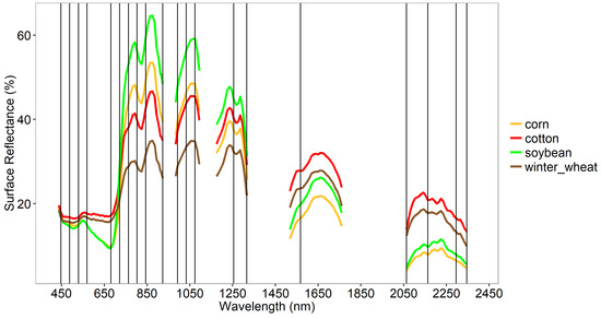
Figure 6.
Optimal hyperspectral narrowbands (OHNBs) in the study of agricultural crops based on Hyperion data of leading world crops in the US. The 20 best hyperspectral narrowbands (HNBs) illustrated with spectral profiles of crops in the critical growth stage. Rice is not included because in the Hyperion images selected, there were no rice spectra in the critical stage.
Comparing these bands with corresponding OHNBs found in earlier literature [54,79], 19 were within 10 nm of previously identified OHNBs, 8 were similar but more than 10 nm from the previously identified bands, and 3 were newly discovered in this study. Table 6 summarizes the importance of each waveband in the study of agricultural crops.
Out of these 30 OHNBs distributed throughout the spectral range (356–2577 nm) (Table 6), the five most important bands included one best band from each of the 5 spectral regions: visible (356 nm to 700 nm), red edge (701 to 760 nm), near-infrared (761 nm to 920 nm, and 1001 nm to 1100 nm), water-absorption (921 nm to 1000 nm), and shortwave infrared (1100 nm to 2577 nm). Thus, the five most important bands were 447, 722, 803, 923, and 2345 nm (Table 7). In selecting the best 10 HNBs, we retained the best 5 and then selected the second best HNB in each of the 5 spectral regions. Since there was only one red-edge band in the 30 most important bands, the next five consisted of two bands from the visible region, one from the near- infrared region, one from the water-absorption region, and one from the shortwave infrared region. Thus, the ten most important bands were 447, 488, 529, 722, 803, 844, 923, 993, 2063, and 2345 nm. There were only two water-absorption region bands in the 30 most important bands, so the next five bands consisted of one band in the visible region, two in the near-infrared region, and two in the shortwave infrared region. The fifteen most important bands, then, were 447, 488, 529, 681, 722, 803, 844, 923, 993, 1033, 1074, 1316, 2063, 2295, and 2345 nm. The next five consisted of one in the visible region, one in the near-infrared, and three in the shortwave infrared region, so the twenty most important bands were 447, 488, 529, 569, 681, 722, 763, 803, 844, 923, 993, 1033, 1074, 1255, 1316, 1568, 2063, 2163, 2295, and 2345 nm. The remaining ten bands were in the shortwave infrared region. The twenty-five most important bands were 447, 488, 529, 569, 681, 722, 763, 803, 844, 923, 993, 1033, 1074, 1175, 1255, 1316, 1528, 1568, 1649, 1699, 2063, 2163, 2254, 2295, and 2345 nm. This selection is summarized in Table 7.
3.2. LDA Across Crop Types
LDAs across crop types were run taking the Hyperion data of 5 crops from 11 images in 5 AEZs, using the data listed in Table 3 and illustrated for a few sample locations in Figure 3. LDA was run for each of the 11 Hyperion images taking 5, 10, 15, 20, 25, and 30 OHNBs (Table 6 and Table 7) resulting in overall accuracy plots depicted in Figure 7, Figure 8, Figure 9, Figure 10 and Figure 11. For example, for Hyperion Image 1 in AEZ 7 (Table 3), overall classification accuracies from 5, 10, 15, 20, 25, and 30 HNBs were 80.8%, 88.5%, 100%, 100%, 100%, and 100% respectively for differentiating corn in the critical growth stage and rice in the early mid growth stage, the two crops and growth stages found in this image (Figure 9). For Hyperion Image 2 in AEZ 7 (Table 3), overall accuracies were 95.2%, 90.5%, 95.2%, 95.2%, 95.2%, and 95.2% respectively for differentiating corn in the critical growth stage and rice in the late growth stage (Figure 9).
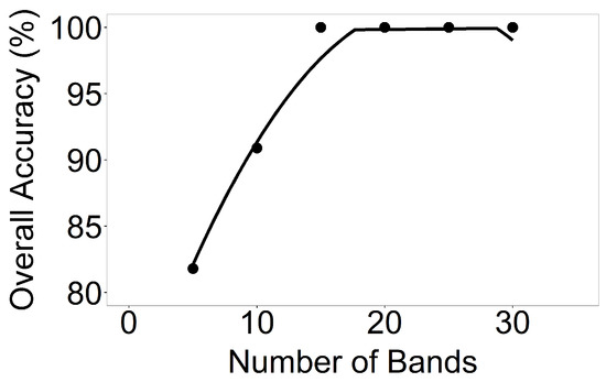
Figure 7.
Number of hyperspectral narrowbands versus classification accuracies of crop types in AEZ 5. Number of hyperspectral narrowbands versus classification accuracies based on LDA of crop types for AEZ 5.
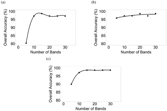
Figure 8.
Number of hyperspectral narrowbands versus classification accuracies of crop types in AEZ 6. Number of hyperspectral narrowbands versus classification accuracies based on linear discriminant analysis (LDA) of crop types for (a) AEZ 6 Image 1; (b) AEZ 6 Image 2; and (c) AEZ 6 Image 3.
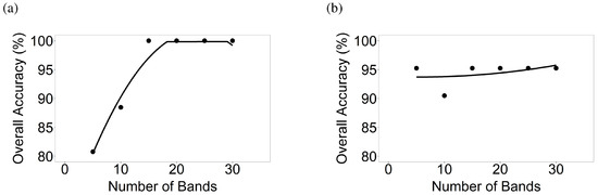
Figure 9.
Number of hyperspectral narrowbands versus classification accuracies of crop types in AEZ 7. Number of hyperspectral narrowbands versus classification accuracies based on LDA of crop types for (a) AEZ 7 Image 1 and (b) AEZ 7 Image 2.
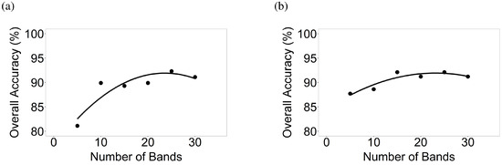
Figure 10.
Number of hyperspectral narrowbands versus classification accuracies of crop types in AEZ 9. Number of hyperspectral narrowbands versus classification accuracies based on LDA of crop types for (a) AEZ 9 Image 1 and (b) AEZ 9 Image 2.
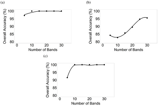
Figure 11.
Number of hyperspectral narrowbands versus classification accuracies of crop types in AEZ 10. Number of hyperspectral narrowbands versus classification accuracies based on LDA of crop types for (a) AEZ 10 Image 1; (b) AEZ 10 Image 2; and (c) AEZ 10 Image 3.
The study area in AEZ 6 (Figure 1) is dominated by corn and soybeans. There were three Hyperion images for this area (Table 3). The overall accuracies for Hyperion Image 1 using 5, 10, 15, 20, 25, and 30 HNBs in classifying corn versus soybean, both in the critical growth stage, were 80.3%, 97.1%, 98.6%, 97.1%, 97.1%, and 97.1% respectively (Figure 8). For Image 2, overall accuracies were 95.8%, 97.2%, 97.2%, 98.6%, 97.2%, and 98.6% respectively for differentiating corn in the late stage and soybean in the early mid stage (Figure 8). For Image 3, overall accuracies were 89.9%, 97.1%, 98.6%, 98.6%, 98.6%, and 98.6% respectively for differentiating corn and soybean, both in the critical growth stage (Figure 8).
In most cases, where 2 crops were involved, fifteen bands were sufficient to reach optimal classification accuracy (Figure 7, Figure 8, Figure 9, Figure 10 and Figure 11). A more complex case is in AEZ 9 (Figure 1) where there were 4 crops (corn, cotton, soybean, and winter wheat). For Hyperion Image 1, overall classification accuracies from 5, 10, 15, 20, 25, and 30 bands were 81.1%, 89.9%, 89.3%, 89.9%, 92.3%, and 91.1% respectively for differentiating corn in the maturing and senescence stage, cotton in the critical stage, soybean in the late stage, and winter wheat in the emergence and very early vegetative stage (Figure 10). For Image 2, overall accuracies were 87.7%, 88.6%, 92.1%, 91.2%, 92.1%, and 91.2% respectively for differentiating corn in the late stage, soybean in the early mid stage, and winter wheat in the maturing and senescence stage (Figure 10). In such complex cases, more than fifteen bands are needed for optimal classification.
3.3. LDA Across Growth Stages
LDAs across growth stages were run for the 5 crops in various growth stages using 99 images in 7 AEZs (Table 3). Training and validation data are listed in Table 5, and example HISA are illustrated in Figure 4. LDAs were run for various crop growth stages (Table 5) of various crops, based on what was present in a given Hyperion image, resulting in overall accuracies depicted in Figure 12.
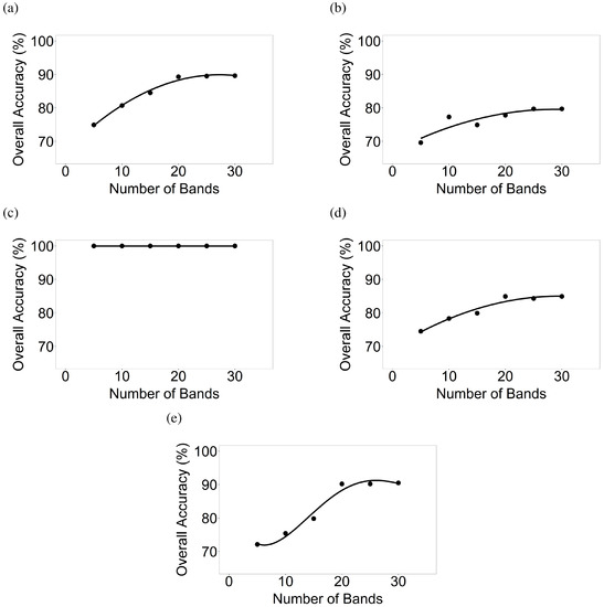
Figure 12.
Number of hyperspectral narrowbands versus classification accuracies of crop growth stages. Number of hyperspectral narrowbands versus classification accuracies determined using discriminant analyses for 6 distinct growth stages, where present, of (a) corn; (b) cotton; (c) rice; (d) soybean; and (e) winter wheat.
For the corn growth stages, overall classification accuracies from 5, 10, 15, 20, 25, and 30 bands were 74.9%, 80.7%, 84.5%, 89.3%, 89.5%, and 89.6% respectively when differentiating six growth stages. For soybean growth stages, accuracies using 5, 10, 15, 20, 25, and 30 bands were 74.5%, 78.3%, 79.9%, 84.9%, 84.3%, and 84.9% respectively. Similarly, discriminant analyses were also run for cotton, rice, and winter wheat for differentiating growth stages (Figure 12). Overall accuracies (excluding rice which was always at 100%) with 5, 10, 15, 20, 25, and 30 bands varied between 69.6–74.9%, 75.4–80.7%, 74.9–84.5%, 77.8–90.2%, 79.7–90.2%, and 79.7–90.5% respectively. Across crops, optimal overall accuracies in separating growth stages were often obtained when 15–20 HNBs were used (Figure 12).
3.4. Image Classification Using Support Vector Machine
All 11 Hyperion images (Table 3) from the 5 AEZs (Figure 1) used for crop type discriminant analyses were classified to separate crop types using SVM and training and validation data listed in Table 4. Fifteen optimal HNBs (Table 7; Figure 6) were used for Hyperion image classification. Illustrations of AEZ 9 Image 1 separating corn, cotton, soybean, and winter wheat using 15 and 30 bands are shown in Figure 13 and Figure 14 respectively. Using 15 bands, this image had an overall accuracy of 86.3% for differentiating corn, cotton, soybean, winter wheat, and other. The producer’s and user’s accuracies were 75.0% and 81.8% respectively for corn, 25.0% and 50.0% respectively for cotton, 70.2% and 67.4% respectively for soybean, and 82.2% and 92.5% respectively for winter wheat. Accuracies for cotton increased substantially to 75.0% and 85.7% respectively using 30 bands.
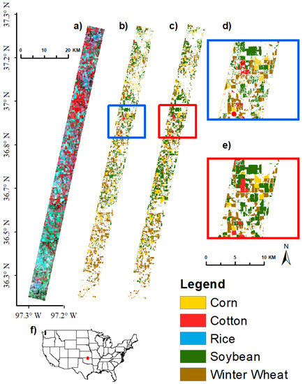
Figure 13.
Crop type classification results for AEZ 9 Image 1 using 15 bands. Crop type image classification results using support vector machine (SVM) supervised classification in GEE for Agroecological Zone (AEZ) 9, EO-1 Hyperion Image 1 using 15 hyperspectral narrowbands. (a) EO-1 Hyperion Image False Color Composite, RGB: 844, 569, 529 nm; (b) SVM classification results using 15 bands; (c) USDA CDL reference data; (d) close-up of SVM results, extent indicated by red box in (b); (e) close-up of CDL reference data, extent indicated by red box in (c); (f) locator map; red rectangle shows location of Hyperion image.
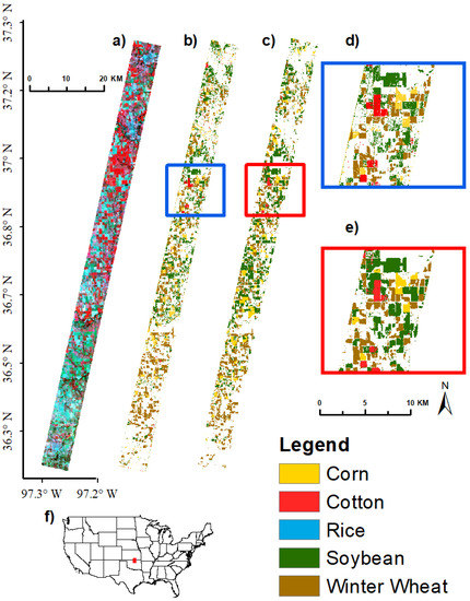
Figure 14.
Crop type classification results for AEZ 9 Image 1 using 30 bands. Crop type image classification results using SVM supervised classification in GEE for Agroecological Zone (AEZ) 9, EO-1 Hyperion Image 1 using 30 hyperspectral narrowbands. (a) EO-1 Hyperion Image False Color Composite, RGB: 844, 569, 529 nm; (b) SVM classification results using 30 bands; (c) USDA CDL reference data; (d) close-up of SVM results, extent indicated by red box in (b); (e) close-up of CDL reference data, extent indicated by red box in (c); (f) locator map; red rectangle shows location of Hyperion image.
A similar process was used to classify the other 10 Hyperion images (Table 3) using the training data listed in Table 4. This resulted in overall accuracies that varied from 75.5 to 95.4%, with most above 90% (Table 8). The producer’s accuracies of crops were: corn 75–98% (errors of omissions 2–25%), cotton 25–100% (0–75%), rice 68.8–92.3% (7.7–31.2%), soybeans 59.1– 95.7% (4.3–40.9%), and winter wheat 37–87.5% (12.5–63%) (Table 8). Most accuracies (overall, producer’s, and user’s were in the 80 to 90% range using 15 OHNBs (Table 8). When these accuracies were low, it implied that a higher number of HNBs was required. For example, the producer’s accuracies of cotton in AEZ 9, went up from 25% with 15 HNBs to 75% with 30 HNBs (Table 8).
Table 8.
Accuracies achieved in classifying crop types using Hyperion data. Summary of image classification results for 11 Hyperion images, using support vector machine (SVM) to classify crop types with 15 optimal hyperspectral narrowbands. AEZ = Agroecological Zone.
4. Discussion
Over 70,000 EO-1 Hyperion images collected from 2001 to 2016 throughout the world are freely available at the USGS EarthExplorer [91]. They provide a great opportunity to conduct various global studies, but are rarely used. The Hyperspectral Imaging Spectral library of Agricultural crops (HISA) developed for 5 principal crops (e.g., Figure 3) during their various distinct growth stages (e.g., Figure 4) across several AEZs in the US (Figure 1) using Hyperion, the first public spaceborne hyperspectral sensor, is unique and unprecedented. The research first established 30 OHNBs (Table 6) to study agriculture and found that 63% of bands were within 10 nm from bands found to be optimal by [54,79] using field spectroradiometer and Hyperion data. Since these overlapping or adjoining bands are nearly 99% correlated, there is a strong match between this finding and earlier findings by [54,79]. Earlier studies [29,55,92,93,94] have demonstrated the value of these and similar OHNBs (Table 6) in a wide array of cropland studies. For example, the bands around 447 nm, 488 nm, 529 nm, and 569 nm are useful for estimating nitrogen and thus pigment content, as well as assessing light use efficiency and stress levels (Table 6). Reflectance at 519 nm and 569 nm were found to be important for rice biomass [95]. Reflectance around 681 nm and around 763 nm can be used to estimate leaf area index and biomass. Additionally, reflectance at 680 nm is important for chlorophyll estimation [69]. Similarly, reflectance at 670 nm was found to be important for estimating dry biomass for several crop types [96]. Reflectance at 755 nm is considered important for biomass [97]. These bands are also useful for crop type differentiation. Bands around 722 nm are important for assessing stress and chlorophyll content. The 803 nm band indicates water absorption, as does 1175 nm. The bands around 844 nm and 923 nm are also important for estimating leaf area index and biomass. Reflectance around 993 nm is influenced by moisture, biomass, and protein content. Bands around 1033 nm and 1074 nm can be used to estimate biomass and pigment content. They are particularly useful for crop type differentiation. Bands around 1215 nm, 1255 nm, and 1316 nm are useful for water band indices and estimating biomass, as are bands near 1528 nm and 1568 nm. Reflectance around 1609 nm and 1649 nm can be used to assess heavy metal stress. The band around 1609 nm is useful for estimating lignin, biomass, starch, and moisture content. The bands at 1760 nm and 2063 nm are water absorption bands. Reflectance at 2204 nm is influenced by structural elements such as lignin and cellulose, as well as sugar, starch, and protein content. This band is also important for assessing heavy metal stress. The 2254 nm band can be used to estimate moisture and biomass. The band at 2295 nm is sensitive to stress levels. Lastly, reflectance around 2345 nm can help estimate cellulose, lignin, starch, protein, and nitrogen content. In this study too, an overwhelming number of the above bands appeared as OHNBs (Table 6). Additionally, four of the seven bands selected in this study that fall within the spectral range of CHRIS PROBA Mode 4 [98] are similar to the bands in Mode 4, specifically designed for vegetation studies (Table 6). This further re-affirms the value of these OHNBs (Table 6 and Table 7) for studying a wide array of crop characteristics, through a comprehensive study using 99 Hyperion images throughout several AEZs in the US for five crops in various crop growth stages.
This study also found three new important HNBs, centered at: 803, 1215, and 1316 nm. These differences between studies may be due to research being conducted on different crops and in different areas. For example, Thenkabail’s team conducted their study on eight leading crops (wheat, corn, rice, barley, soybean, pulses, cotton, and alfalfa) using field spectroradiometer and Hyperion hyperspectral data over Africa, the Middle East, Central Asia, and India [54]. The OHNBs selected depend heavily on the research goal, for example crop classification and biomass estimation; for these different objectives, various researchers [29,55,93] have confirmed that it is important to identify the redundant HNBs and eliminate them to overcome data redundancy and overcome Hughes’ phenomenon. The outcome of this research contributes to this effort with a focus on crop type and growth stage classification.
In Figure 7, Figure 8, Figure 9, Figure 10, Figure 11 and Figure 12, we illustrate how overall accuracies for crop type classifications increase with an increasing number of bands. However, in most cases accuracies asymptote around 15–20 bands. In complex cases (e.g., 4 or more crops in a single image) the accuracies keep increasing even up to 25 to 30 bands. However, beyond 30 bands increase in accuracies is negligible in almost all cases and any small increase is often a mathematical artifact. Using 15 of the 30 OHNBs (Table 6 and Table 7), we were able to map crop types with overall, producer’s and user’s accuracies of 80–90% or higher in an overwhelming number of cases. In most images, the optimal classification was achieved using 15 bands. These bands collectively were able to differentiate crop types due to differences in pigment content, biomass, water content, structural elements, and stress levels. Other research [54,79] has shown that the 763 nm and 1699 nm bands are important for crop type differentiation. Although these were important in this study, they were not in the 15 most important bands selected.
Crop growth stages were also able to be differentiated using at most 30 bands. In most cases, 20 bands were sufficient. Accuracies also increase substantially when we are separating fewer growth stages. For example, when we used 3 consolidated growth stages of early, mid, and late (results not presented here), we found the overall accuracies increased by 7% for corn, 11% for cotton, 10% for soybean, and 1% for winter wheat; there was no difference for rice.
Crop types were differentiated using SVM image classifications conducted on Hyperion images in GEE. High accuracies (around 90%, in most cases; Table 8) were obtained by using only 15 HNBs. This allows for removal of a large number of redundant Hyperion bands, resulting in overcoming data redundancy, and Hughes’ phenomenon or the curse of high dimensionality.
SVMs are powerful classification algorithms. However, they can be computationally intensive and time-consuming due to the cross-validation needed for parameter optimization. We compared RF results with SVM results for a few images, and found that we had lower accuracies and more omission errors with RF than with SVM. Thus, despite greater computation intensity, we used SVM. Models were not applied across images because variability across AEZs and years would add substantial noise. This needs to be explored more thoroughly in future studies.
Methods and OHNBs established in this study can aid crop type and growth stage differentiation using future hyperspectral sensors. Conducting such analyses at global extents using cloud-computing can enable decision-making to address global food security issues in a timely manner.
5. Conclusions
Earth Observing-1 (EO-1) Hyperion images were used to study five globally dominant crops (corn, cotton, rice, soybean, and winter wheat) and their growth stages in the United States, where they occupy about 75% of all the cropland areas occupied by the principal crops, using the Google Earth Engine (GEE) cloud computing platform. Hyperion images from various agroecological zones (AEZs) were used to compile a first-of-its-kind Hyperspectral Imaging Spectral library of Agricultural crops (HISA) of these five crop types for the United States. To reduce data dimensionality, autocorrelation, and issues related to the Hughes’ Phenomenon or curse of high dimensionality, we used principal component analyses to select 30 optimal hyperspectral narrowbands (OHNBs), allowing us to overcome data redundancy. Overwhelmingly, 15–20 hyperspectral narrowbands (HNBs) achieved about 90% overall, producer’s, and user’s accuracies in classifying crop types and/or crop growth stages using linear discriminant analysis (LDA) and/or the support vector machine (SVM) classifier. However, when complex situations occurred (e.g., 4 or more crops within a Hyperion image), up to 30 HNBs were required to best classify and characterize these crops. The study showed that hyperspectral satellite imagery, when analyzed on the GEE cloud computing platform using machine learning algorithms like SVMs, provides a fast and accurate means of classifying agricultural crops and their characteristics such as crop growth stages, which can help advance global food security information derived from satellites. This study makes a significant contribution to studying agricultural crops using data from upcoming hyperspectral missions, and in advancing the compilation of a novel global hyperspectral imaging spectral-library of agricultural-crops (GHISA; www.usgs.gov/WGSC/GHISA) [99].
Author Contributions
Conceptualization, Prasad Thenkabail; Formal analysis, Itiya Aneece; Methodology, Itiya Aneece and Prasad Thenkabail; Supervision, Prasad Thenkabail; Writing—original draft, Itiya Aneece and Prasad Thenkabail.
Funding
This research was funded by the USGS Mendenhall Postdoctoral Fellowship.
Acknowledgments
The authors thank the Mendenhall Postdoctoral Fellowship through the Western Geographic Science Center, US Geological Survey for funding this research. Additionally, we thank the internal reviewers at the USGS for providing feedback that has much strengthened the manuscript. Likewise, we thank external reviewers for their constructive comments and suggestions.
Conflicts of Interest
The authors declare no conflict of interest.
References
- Odegard, I.; van der Voet, E. The future of food—Scenarios and the effect on natureal resource use in agriculture in 2050. Ecol. Econ. 2014, 97, 51–59. [Google Scholar] [CrossRef]
- Kruse, F.; Baugh, W.; Perry, S. Validation of DigitalGlobe WorldView-3 Earth imaging satellite shortwave infrared bands for mineral mapping. J. Appl. Remote Sens. 2015, 9, 096044-1–096044-17. [Google Scholar] [CrossRef]
- Lambert, M.; Traore, P.; Blaes, X.; Baret, P.; Defourny, P. Estimating smallholder crops production at village level from Sentinel-2 time series in Mali’s cotton belt. Remote Sens. Environ. 2018, 216, 647–657. [Google Scholar] [CrossRef]
- Jarolmasjed, S.; Sankaran, S.; Kalcsits, L.; Khot, L. Proximal hyperspectral sensing of stomatal conductance to monitor the efficacy of exogenous abscisic acid applications in apple trees. Crop Protect. 2018, 109, 42–50. [Google Scholar] [CrossRef]
- McDowell, M.; Kruse, F. Enhanced compositional mapping through integrated full-range spectral analysis. Remote Sens. 2016, 8, 757. [Google Scholar] [CrossRef]
- Sun, J.; Shi, S.; Gong, W.; Yang, J.; Du, L.; Song, S.; Chen, B.; Zhang, Z. Evaluation of hyperspectral LiDAR for monitoring rice leaf nitrogen by comparison with multispectral LiDAR and passive spectrometer. Nat. Sci. Rep. 2017, 7, 9. [Google Scholar] [CrossRef] [PubMed]
- Wu, M.; Huang, W.; Niu, Z.; Wang, Y.; Wang, C.; Li, W.; Hao, P.; Yu, B. Fine crop mapping by combining high spectral and high spatial resolution remote sensing data in complex heterogeneous areas. Comput. Electron. Agric. 2017, 139, 1–9. [Google Scholar] [CrossRef]
- Marshall, M.; Thenkabail, P. Advantage of hyperspectral EO-1 Hyperion over multispectral IKONOS, GeoEye-1, WorldView-2, Landsat ETM+, and MODIS vegetation indices in crop biomass estimation. ISPRS J. Photogramm. Remote Sens. 2015, 108, 205–218. [Google Scholar] [CrossRef]
- He, K.; Rocchini, D.; Neteler, M.; Nagendra, H. Benefits of hyperspectral remote sensing for tracking plant invasions. Divers. Distrib. 2011, 17, 381–392. [Google Scholar] [CrossRef]
- Underwood, E.; Ustin, S.; Ramirez, C. A comparison of spatial and spectral image resolution for mapping invasive plants in coastal California. J. Environ. Manag. 2007, 39, 63–83. [Google Scholar] [CrossRef]
- Underwood, E.; Ustin, S.; DiPietro, D. Mapping nonnative plants using hyperspectral imagery. Remote Sens. Environ. 2003, 86, 150–161. [Google Scholar] [CrossRef]
- Carlson, K.; Asner, G.; Hughes, R.; Ostertag, R.; Martin, R. Hyperspectral remote sensing of canopy biodiversity in Hawaiian lowland rainforests. Ecosystems 2007, 10, 536–549. [Google Scholar] [CrossRef]
- Banskota, A.; Wynne, R.; Kayastha, N. Improving within-genus tree species discrimination using the discrete wavelet transform applied to airborne hyperspectral data. Int. J. Remote Sens. 2011, 32, 3551–3563. [Google Scholar] [CrossRef]
- Cho, M.; Mathieu, R.; Asner, G.; Naidoo, L.; van Aardt, J.; Ramoelo, A.; Debba, P.; Wessels, K.; Main, R.; Smit, I.; et al. Mapping tree species composition in South African savannas using an integrated airborne spectral and LiDAR system. Remote Sens. Environ. 2012, 125, 214–226. [Google Scholar] [CrossRef]
- Naidoo, L.; Cho, M.; Mathieu, R.; Asner, G. Classification of savanna tree species, in the Greater Kruger National Park region, by integrating hyperspectral and LiDAR data in a Random Forest data mining environment. ISPRS J. Photogramm. Remote Sens. 2012, 69, 167–179. [Google Scholar] [CrossRef]
- Zhang, J.; Rivard, B.; Sanchez-Azofeifa, A.; Castro-Esau, K. Intra- and inter-class spectral variability of tropical tree species at La Selva, Costa Rica: Implications for species identification using HYDICE imagery. Remote Sens. Environ. 2006, 105, 129–141. [Google Scholar] [CrossRef]
- Shafri, H.; Suhaili, A.; Mansor, S. The performance of maximum likelihood, spectral angle mapper, neural network and decision tree classifiers in hyperspectral image analysis. J. Comput. Sci. 2007, 3, 419–423. [Google Scholar] [CrossRef]
- Andrew, M.; Ustin, S. Spectral and physiological uniqueness of perennial pepperweed (Lepidium latifolium). Weed Sci. 2006, 54, 1051–1062. [Google Scholar] [CrossRef]
- Zomer, R.; Trabucco, A.; Ustin, S. Building spectral libraries for wetlands land cover classification and hyperspectral remote sensing. J. Environ. Manag. 2009, 90, 2170–2177. [Google Scholar] [CrossRef]
- Daughtry, C.; Hunt, E., Jr.; Doraiswamy, P.; McMurtrey, J., III. Remote sensing the spatial distribution of crop residues. Agron. J. 2005, 97, 864–871. [Google Scholar] [CrossRef]
- He, Y.; Mui, A. Scaling up semi-arid grassland biochemical content from the leaf to the canopy level: Challenges and opportunities. Sensors 2010, 10, 11072–11087. [Google Scholar] [CrossRef] [PubMed]
- Beland, M.; Roberts, D.; Peterson, S.; Biggs, T.; Kokaly, R.; Piazza, S.; Roth, K.; Khanna, S.; Ustin, S. Mapping changing distributions of dominant species in oil-contaminated salt marshes of Louisiana using imaging spectroscopy. Remote Sens. Environ. 2016, 182, 192–207. [Google Scholar] [CrossRef]
- Peterson, S.; Roberts, D.; Beland, M.; Kokaly, R.; Ustin, S. Oil detection in the coastal marshes of Louisiana using MESMA applied to band subsets of AVIRIS data. Remote Sens. Environ. 2015, 159, 222–231. [Google Scholar] [CrossRef]
- Kefauver, S.; Penuelas, J.; Ustin, S. Applications of hyeprspectral remote sensing and GIS for assessing forest health and air pollution. In Proceedings of the 2012 IEEE International Geoscience and Remote Sensing Symposium (IGARSS), Munich, Germany, 22–27 July 2012. [Google Scholar]
- Smith, A.; Blackshaw, R. Weed-crop discrimination using remote sensing: A detached leaf experiment. Weed Technol. 2003, 17, 811–820. [Google Scholar] [CrossRef]
- Sahoo, R.; Ray, S.; Manjunath, K. Hyperspectral remote sensing of agriculture. Curr. Sci. 2015, 108, 848–859. [Google Scholar]
- Yang, C.; Everitt, J.; Bradford, J. Yield estimation from hyperspectral imagery using spectral angle mapper (SAM). Trans. ASABE 2008, 51, 729–737. [Google Scholar] [CrossRef]
- Jafari, R.; Lewis, M. Arid land characterization with EO-1 Hyperion hyperspectral data. Int. J. Appl. Earth Obs. Geoinf. 2012, 19, 298–307. [Google Scholar] [CrossRef]
- Thenkabail, P.; Enclona, E.; Ashton, M.; Legg, C.; De Dieu, M. Hyperion, IKONOS, ALI, and ETM+ sensors in the study of African rainforests. Remote Sens. Environ. 2004, 90, 23–43. [Google Scholar] [CrossRef]
- Asner, G.; Heidebrecht, K. Imaging spectroscopy for desertification studies: Comparing AVIRIS and EO-1 Hyperion in Argentina drylands. IEEE Trans. Geosci. Remote Sens. 2003, 41, 1283–1296. [Google Scholar] [CrossRef]
- Oskouei, M.; Babakan, S. Detection of alteration minerals using Hyperion data analysis in Lahroud. J. Indian Soc. Remote Sens. 2016, 44, 713–721. [Google Scholar] [CrossRef]
- Dadon, A.; Ben-Dor, E.; Beyth, M.; Karnieli, A. Examination of spaceborne imaging spectroscopy data utility for stratigraphic and lithologic mapping. J. Appl. Remote Sens. 2011, 5, 053507-1–053507-14. [Google Scholar] [CrossRef]
- Papes, M.; Tupayachi, R.; Martinez, P.; Peterson, A.; Powell, G. Using hyperspectral satellite imagery for regional inventories: A test with tropical emergent trees in the Amazon Basin. J. Veg. Sci. 2010, 21, 342–354. [Google Scholar] [CrossRef]
- Somers, B.; Asner, G. Tree species mapping in tropical forests using multi-temporal imaging spectroscopy: Wavelength adaptive spectral mixture analysis. Int. J. Appl. Earth Obs. Geoinf. 2014, 31, 57–66. [Google Scholar] [CrossRef]
- Somers, B.; Asner, G. Mapping tropical rainforest canopies using multi-temporal spaceborne imaging spectroscopy. Proc. SPIE 2013, 8887, 888704-1–888704-8. [Google Scholar]
- Christian, B.; Krishnayya, N. Classification of tropical trees growing in a sanctuary using Hyperion (EO-1) and SAM algorithm. Curr. Sci. 2009, 96, 1601–1607. [Google Scholar]
- George, R.; Padalia, H.; Kushwaha, S. Forest tree species discrimination in western Himalaya using EO-1 Hyperion. Int. J. Appl. Earth Obs. Geoinf. 2014, 28, 140–149. [Google Scholar] [CrossRef]
- Walsh, S.; McCleary, A.; Mena, C.; Shao, Y.; Tuttle, J.; Gonzalez, A.; Atkinson, R. QuickBird and Hyperion data analysis of an invasive plant species in the Galapagos Islands of Ecuador: Implications for control and land use management. Remote Sens. Environ. 2008, 112, 1927–1941. [Google Scholar] [CrossRef]
- Somers, B.; Asner, G. Multi-temporal hyperspectral mixture analysis and feature selection for invasive species mapping in rainforests. Remote Sens. Environ. 2013, 136, 14–27. [Google Scholar] [CrossRef]
- Huemmrich, K.; Gamon, J.; Tweedie, C.; Campbell, P.; Landis, D.; Middleton, E. Arctic tundra vegetation functional types based on photosynthetic physiology and optical properties. IEEE J. Sel. Top. Appl. Earth Obs. Remote Sens. 2013, 6, 265–275. [Google Scholar] [CrossRef]
- Mielke, C.; Boesche, N.; Rogass, C.; Kaufmann, H.; Gauert, C.; de Wit, M. Spaceborne mine waste minerology monitoring in South Africa, applications for modern push-broom missions: Hyperion/ OLI and EnMAP/ Sentinel-2. Remote Sens. 2014, 6, 6790–6816. [Google Scholar] [CrossRef]
- Sims, N.; Culvenor, D.; Newnham, G.; Coops, N.; Hopmans, P. Towards the operational use of satellite hyperspectral image data for mapping nutrient status and fertilizer requirements in Australian plantation forests. IEEE J. Sel. Top. Appl. Earth Obs. Remote Sens. 2013, 6, 320–328. [Google Scholar] [CrossRef]
- Zhang, Q.; Middleton, E.; Cheng, Y.; Landis, D. Variations of foliage chlorophyll fAPAR and foliage non-chlorophyll fAPAR (fAPARchl, fAPARnon-chl) at the Harvard Forest. IEEE J. Sel. Top. Appl. Earth Obs. Remote Sens. 2013, 6, 2254–2264. [Google Scholar] [CrossRef]
- Roberts, D.; Dennison, P.; Gardner, M.; Hetzel, Y.; Ustin, S.; Lee, C. Evaluation of the potential of Hyperion for fire danger assessment by comparison to the airborne visible/ infrared imaging spectrometer. IEEE Trans. Geosci. Remote Sens. 2003, 41, 1297–1310. [Google Scholar] [CrossRef]
- Mitri, G.; Gitas, I. Mapping postfire vegetation recovery using EO-1 Hyperion imagery. IEEE Trans. Geosci. Remote Sens. 2010, 48, 1613–1618. [Google Scholar] [CrossRef]
- Bannari, A.; Staenz, K.; Champagne, C.; Khurshid, K. Spatial variability mapping of crop residue using Hyperion (EO-1) hyperspectral data. Remote Sens. 2015, 7, 8107–8127. [Google Scholar] [CrossRef]
- Sonmez, N.; Slater, B. Measuring intensity of tillage and plant residue cover using remote sensing. Eur. J. Remote Sens. 2016, 49, 121–135. [Google Scholar] [CrossRef]
- Bhojaraja, B.E.; Shetty, A.; Nagaraj, M.K.; Manju, P. Age-based classification of arecanut crops: A case study of Channagiri, Karnataka, India. Geocarto Int. 2015, 1–11. [Google Scholar] [CrossRef]
- Breunig, F.; Galvao, L.; Formaggio, A.; Epiphanio, J. Classification of soybean varieties using different techniques: Case study with Hyperion and sensor spectral resolution simulations. J. Appl. Remote Sens. 2011, 5, 053533-1–053533-15. [Google Scholar] [CrossRef]
- Pan, Z.; Huang, J.; Wang, F. Multi range spectral feature fitting for hyperspectral imagery in extracting oilseed rape planting area. Int. J. Appl. Earth Obs. Geoinf. 2013, 25, 21–29. [Google Scholar] [CrossRef]
- Lamparelli, R.; Johann, J.; Dos Santos, E.; Esquerdo, J.; Rocha, J. Use of data mining and spectral profiles to differentiate condition after harvest of coffee plants. Eng. Agric. Jaboticabal 2012, 32, 184–196. [Google Scholar] [CrossRef]
- Moharana, S.; Dutta, S. Spatial variability of chlorophyll and nitrogen content of rice from hyperspectral imagery. ISPRS J. Photogramm. Remote Sens. 2016, 122, 17–29. [Google Scholar] [CrossRef]
- Houborg, R.; McCabe, M.; Angel, Y.; Middleton, E. Detection of chlorophyll and leaf area index dynamics from sub-weekly hyperspectral imagery. Proc. SPIE 2016, 9998. [Google Scholar] [CrossRef]
- Thenkabail, P.; Mariotto, I.; Gumma, M.; Middleton, E.; Landis, D.; Huemmrich, K. Selection of hyperspectral narrowbands (HNBs) and composition of hyperspectral two band vegetation indices (HVIs) for biophysical characterization and discrimination of crop types using field reflectance and Hyperion/ EO-1 data. IEEE J. Sel. Top. Appl. Earth Obs. Remote Sens. 2013, 6, 427–439. [Google Scholar] [CrossRef]
- Mariotto, I.; Thenkabail, P.; Huete, A.; Slonecker, T.; Platonov, A. Hyperspectral versus multispectral crop-productivity modeling and type discrimination for the HyspIRI mission. Remote Sens. Environ. 2013, 139, 291–305. [Google Scholar] [CrossRef]
- Gorelick, N.; Hancher, M.; Dixon, M.; Ilyushchenko, S.; Thau, D.; Moore, R. Google Earth Engine: Planetary-scale geospatial analysis for everyone. Remote Sens. Environ. 2017, 202, 18–27. [Google Scholar] [CrossRef]
- National Academies of Sciences, Engineering and Medicine. Thriving on Our Changing Planet: A Decadal Strategy for Earth Observation from Space; The National Academies Press: Washington, DC, USA, 2018. [Google Scholar] [CrossRef]
- Eckardt, A.; Horack, J.; Lehmann, F.; Krutz, D.; Drescher, J.; Whorton, M.; Soutullo, M. DESIS (DLR Earth Sensing Imaging Spectrometer for the ISS-MUSES platform). In Proceedings of the 2015 IEEE International Geoscience and Remote Sensing Symposium (IGARSS), Milan, Italy, 26–31 July 2015; pp. 1457–1459. [Google Scholar] [CrossRef]
- FAO—Food and Agriculture Organization of the United Nations. GAEZ-–Global Agro-Ecological Zones; FAO: Rome, Italy, 2018. [Google Scholar]
- NASS. USDA National Agricultural Statistics Service Cropland Data Layer. 2014. Available online: https://nassgeodata.gmu.edu/CropScape/ (accessed on 28 September 2018).
- NASS. USDA CropScape and Cropland Data Layer-Metadata; Technical Report; United States Department of Agriculture, National Agricultural Statistics Service, NASS Marketing and Information Services Office: Washington, DC, USA, 2018.
- NASS. United States Department of Agriculture: National Agricultural Statistics Service. 2017. Available online: https://www.nass.usda.gov/ (accessed on 28 September 2018).
- NASS. USDA Crop Production 2017 Summary: January 2018; Technical Report; United States Department of Agriculture, National Agricultural Statistics Service, NASS Marketing and Information Services Office: Washington, DC, USA, 2018.
- Aneece, I.; Thenkabail, P. Spaceborne hyperspectral EO-1 Hyperion data pre-processing: Methods, approaches, and algorithms. In Hyperspectral Remote Sensing of Vegetation; Taylor and Francis Inc./CRC Press: Boca Raton, FL, USA, 2018. [Google Scholar]
- Pervez, W.; Uddin, V.; Khan, S.; Khan, J. Satellite-based land use mapping: Comparative analysis of Landsat-8, Advanced Land Imager, and big data Hyperion imagery. J. Appl. Remote Sens. 2016, 10, 026004-1–026004-20. [Google Scholar] [CrossRef]
- Das, P.; Seshasai, M. Multispectral sensor spectral resolution simulations for generation of hyperspectral vegetation indices for Hyperion data. Geocarto Int. 2015, 30, 686–700. [Google Scholar] [CrossRef]
- Farifteh, J.; Nieuwenhuis, W.; Garcia-Melendez, E. Mapping spatial variations of iron oxide by-product minerals from EO-1 Hyperion. Int. J. Remote Sens. 2013, 34, 682–699. [Google Scholar] [CrossRef]
- San, B.; Suzen, M. Evaluation of cross-track illumination in EO-1 Hyperion imagery for lithological mapping. Int. J. Remote Sens. 2011, 32, 7873–7889. [Google Scholar] [CrossRef]
- Datt, B.; McVicar, T.; Van Niel, T.; Jupp, D.; Pearlman, J. Preprocessing EO-1 Hyperion hyperspectral data to support the application of agricultural indexes. IEEE Trans. Geosci. Remote Sens. 2003, 41, 1246–1259. [Google Scholar] [CrossRef]
- Gueymard, C. SMARTS2, a Simple Model of the Atmospheric Radiative Transfer of Sunshine: Algorithms and Performance Assessment; Technical Report FSEC-PF-270-95; Florida Solar Energy Center, University of Central Florida: Cocoa, FL, USA, 1995. [Google Scholar]
- Gueymard, C. Parameterized transmittance model for direct beam and circumsolar spectral irradiance. Sol. Energy 2001, 71, 325–346. [Google Scholar] [CrossRef]
- Seidel, F.; Kokhanovsky, A.; Schaepman, M. Fast and simple model for atmospheric radiative transfer. Atmos. Meas. Tech. 2010, 3, 1129–1141. [Google Scholar] [CrossRef]
- Chavez, P., Jr. Image-based atmospheric corrections- revisited and improved. Photogramm. Eng. Remote Sens. 1996, 62, 1025–1036. [Google Scholar]
- Gopinathan, K.; Polokoana, P. Estimation of hourly beam and diffuse solar radiation. Sol. Wind Technol. 1986, 3, 223–229. [Google Scholar] [CrossRef]
- NOAA. NOAA Integrated Surface Database. 2017. Available online: https://www.ncdc.noaa.gov/isd (accessed on 8 December 2016).
- Abatzoglou, J. Development of gridded surface meteorological data for ecological applications and modelling. Int. J. Climatol. 2013, 33, 121–131. [Google Scholar] [CrossRef]
- NASS. United States Department of Agriculture National Agricultural Statistics Service, Research and Science: Cropscape and Cropland Data Layers- FAQs. 2018. Available online: https://www.nass.usda.gov/Research_and_Science/Cropland/sarsfaqs2.php (accessed on 28 September 2018).
- Stevens, A.; Ramirez-Lopez, L. Package ‘Prospectr’. Technical Report. 2015. Available online: https://cran.r-project.org/web/packages/prospectr/prospectr.pdf (accessed on 8 June 2018).
- Thenkabail, P.; Gumma, M.; Telaguntla, P.; Mohammed, I. Hyperspectral remote sensing of vegetation and agricultural crops. Photogramm. Eng. Remote Sens. 2014, 80, 697–709. [Google Scholar]
- Mulla, D. Twenty five years of remote sensing in precision agriculture: Key advances and remaining knowledge gaps. Biosyst. Eng. 2013, 114, 358–371. [Google Scholar] [CrossRef]
- Bajwa, S.; Kulkarni, S.; Lyon, J.; Huete, A. Hyperspectral data mining. In Hyperspectral Remote Sensing of Vegetation; Thenkabail, P., Ed.; CRC Press, Taylor and Francis Group: Boca Raton, FL, USA, 2011; pp. 93–120. [Google Scholar]
- Laparra, V.; Malo, J.; Camps-Valls, G. Dimensionality reduction via regression in hyperspectral imagery. IEEE J. Sel. Top. Signal Process. 2015, 9, 1026–1036. [Google Scholar] [CrossRef]
- Ding, C.; He, X.; Zha, H.; Simon, H. Adaptive dimension reduction for clustering high dimensional data. In Proceedings of the International Conference on Data Mining, Maebashi City, Japan, 9–12 December 2002; pp. 1–8. [Google Scholar]
- Binol, H.; Ochilov, S.; Alam, M.; Bai, A. Target oriented dimensionality reduction of hyperspectral data by Kernel Fukunaga-Koontz Transform. Opt. Lasers Eng. 2017, 89, 123–130. [Google Scholar] [CrossRef]
- Chang, P.; Yang, J.; Den, W.; Wu, C. Characterizing and locating air pollution sources in a complex industrial district using optical remote sensing technology and multivariate statistical modeling. Environ. Sci. Pollut. Res. 2014, 21, 10852–10866. [Google Scholar] [CrossRef]
- Shahdoosti, H.; Mirzapour, F. Spectral-spatial feature extraction using orthogonal linear discriminant analysis for classification of hyperspectral data. Eur. J. Remote Sens. 2017, 50, 111–124. [Google Scholar] [CrossRef]
- Maxwell, A.; Warner, T.; Fang, F. Implementation of machine-learning classification in remote sensing: An applied review. Int. J. Remote Sens. 2018, 39, 2784–2817. [Google Scholar] [CrossRef]
- Maxwell, A.; Warner, T.; Strager, M.; Conley, F.; Sharp, A. Assessing machine-learning algorithms and image- and LiDAR-derived variables for GEOBIA classification of mining and mine reclamation. Int. J. Remote Sens. 2015, 36, 954–978. [Google Scholar] [CrossRef]
- Xiong, J.; Thenkabail, P.; Tilton, J.; Gumma, M.; Teluguntla, P.; Oliphant, A.; Congalton, R.; Yadav, K.; Gorelick, N. Nominal 30-m cropland extent map of continental Africa by integration pixel-based and object-based algorithms using Sentinel-2 and Landsat-8 data on Google Earth Engine. Remote Sens. 2017, 9, 1065. [Google Scholar] [CrossRef]
- Hsu, C.; Chang, C.; Lin, C. A Practical Guide to Support Vector Classification. 2010, pp. 1–10. Available online: https://www.csie.ntu.edu.tw/~cjlin/papers/guide/guide.pdf (accessed on 24 January 2013).
- USGS. USGS EarthExplorer—Home. 2018. Available online: https://earthexplorer.usgs.gov/ (accessed on 28 September 2018).
- Suarez, L.; Apan, A.; Werth, J. Detection of phenoxy herbicide dosage in cotton crops through the analysis of hyperspectral data. Int. J. Remote Sens. 2017, 38, 6528–6553. [Google Scholar] [CrossRef]
- Marshall, M.; Thenkabail, P. Biomass modeling of four leading world crops using hyperspectral narrowbands in support of HyspIRI mission. Photogramm. Eng. Remote Sens. 2014, 80, 757–772. [Google Scholar] [CrossRef]
- Nugent, P.; Shaw, J.; Jha, P.; Scherrer, B.; Donelick, A.; Kumar, V. Discrimination of herbicide-resistant kochia with hyperspectral imaging. J. Appl. Remote Sens. 2018, 12, 016037-1–016037-10. [Google Scholar] [CrossRef]
- Feng, H.; Jiang, N.; Huang, C.; Fang, W.; Yang, W.; Chen, G.; Xiong, L.; Liu, Q. A hyperspectral imaging system for an accurate prediction of the above-ground biomass of individual rice plants. Rev. Sci. Instrum. 2013, 84, 095107-1–095107-10. [Google Scholar] [CrossRef] [PubMed]
- Liu, J.; Miller, J.; Pattey, E.; Haboudane, D.; Strachan, I.; Hinther, M. Monitoring crop biomass accumulation using multi-temporal hyperspectral remote sensing data. In Proceedings of the IEEE International Geosicence and Remote Sensing Symposium, Anchorage, AK, USA, 20–24 September 2004; Volume 3, pp. 1637–1640. [Google Scholar]
- Mutanga, O.; Skidmore, A. Narrow band vegetation indices overcome the saturation problem in biomass estimation. Int. J. Remote Sens. 2004, 25, 3999–4014. [Google Scholar] [CrossRef]
- Cutter, M.; Kellar-Bland, H. CHRIS Data Format; Technical Report SmarTeam 0114848; Surrey Satellite Technology LTD- Chris Operations: Guildford, UK, 2008. [Google Scholar]
- Thenkabail, P.; Aneece, I.; Teluguntla, P.; Oliphant, A.; Foley, D.; Williamson, D. Global Hyperspectral Imaging Spectroscopy of Agricultural-Crops & Vegetation (GHISA). 2019. Available online: www.usgs.gov/WGSC/GHISA (accessed on 30 May 2018).
© 2018 by the authors. Licensee MDPI, Basel, Switzerland. This article is an open access article distributed under the terms and conditions of the Creative Commons Attribution (CC BY) license (http://creativecommons.org/licenses/by/4.0/).