Abstract
A high-resolution three-dimensional (3D) image reconstruction method for a spinning target is proposed in this paper and the anisotropy is overcome by fusing different observation information acquired from the radar network. The proposed method will reconstruct the 3D scattering distribution, and the mapping of the reconstructed 3D image onto the imaging plane is identical to the two-dimensional (2D) imaging result. At first, the range compression and inverse radon transform is employed to produce the 2D image of the spinning target. In addition, the process of mapping the spinning target onto the imaging plane is analyzed and the mapping formulas which are to map the point onto the 2D image plane are derived. After the micro-Doppler signature about which every reconstructed point in 2D imaging result is extracted by the Radon transform, the extended Hough transform is adopted to calculate an important parameter about the micro-Doppler signature, and the 3D image reconstruction model for the spinning target is constructed based on the radar network. Finally, the algorithm for solving the reconstruction model is proposed and the 3D image of the spinning target is obtained. Some simulation results are given to illustrate the effectiveness of the proposed method, and results show that the mean square error (MSE) relatively holds a steady trend when the signal-to-noise ratio (SNR) is higher than −10 dB and the MSE of the reconstructed 3D target image is less than 0.15 when SNR is at the level of −10 dB.
1. Introduction
High-resolution radar imaging based on inverse synthetic aperture radar (ISAR) technology is a significant investigation and recognition measure for air-maneuvering targets and sea-surface targets, and it can extract the shape structure information of the targets [1,2]. Sadjadi proposed a classification method for small boats using polarimetric ISAR imagery [3], and motion-induced distortions in polarimetric ISAR imagery are removed by several enhancement methods. Furthermore, high-resolution two-dimensional (2D) imaging with the wide-band transmitted signal and larger coherent accumulation angle can produce the 2D image which, is the mapping of the air-maneuvering target on the imaging plane [4]. The imaging plane is constituted by the direction of translational motion and radar line of sight (LOS). The mapping result would be different when the target is mapped on the different imaging plane [5]. Therefore, the 2D imaging result could not represent the true information of the target. To overcome this limitation, the high-resolution three-dimensional (3D) imaging which can represent the true characteristic and extract more information about the target has been explored and employed [6]. The commonly known techniques for forming 3D image mainly contain 3D ISAR imaging [7], ISAR movie [8], “snapshot” 3D imaging [9], interferometric ISAR technique [10,11], etc., but most of them are not suitable for the spinning target which possesses translational motion and micromotion.
Recently, many researchers have attempted to address high-resolution 3D imaging for the target with micromotion, and the existing 3D imaging techniques for micromotion target can be classified into two categories, i.e., the nonparametric methods and the parametric methods [12]. Among them, the nonparametric methods fall into the following categories: (1) scattering center trajectory association-based imaging; and (2) interferometric technique. Bai et al. proposed a nonparametric 3D-imaging method based on scattering center trajectory association [13], and the matrix completion method based on the Riemannian manifold optimization was designed. Sun et al. proposed a time-varying interferometric 3D imaging method for space rotating targets based on stepped-frequency chirp signal [14]. In addition, the parametric methods for forming 3D image of micromotion target mainly include 3D imaging of spinning targets based on the fixed scattering center model and imaging of smooth precession cones based on the sliding scattering center model [15,16,17,18]. However, the scattering center trajectory association is not easy to accomplish due to the shadowing effect, limited range resolution, and small angular extent; the interferometric 3D imaging method needs a more complex hardware structure; and the parametric methods have to face a large amount of unknown parameters in imaging the artificial metallic target [19,20,21]. Furthermore, the anisotropy is usually ignored in the process of the 3D imaging for the air target, especially in the monostatic radar system [22]. Therefore, it is necessary for the anisotropy problem to fuse different observation information acquired from a multistatic radar system and to design the corresponding 3D image reconstruction technique for the spinning target based on the multistatic radar system.
Just like a mirror or flat metal sheet may reflect more strongly when viewed straight on than from an oblique angle, the anisotropy is the problem that the scattering intensity is varied as the observation perspective changing and depends on the scattering behavior on observation perspective [23,24]. Kim et al. proposed a general characterization of anisotropy based on a sub-aperture pyramid in synthetic aperture radar (SAR) imagery [25], and how anisotropy attribution might be conducive to the recognition problem is explored. Even though a monostatic radar may observe the air target for a long time, the radar observation perspective is limited and the available scattering information about the target would normally be incomplete [26]. On account of the anisotropy, it is tough for a monostatic radar with the limited scattering information to reconstruct the whole 3D scattering distribution of the air target. One of method to overcome the anisotropy is to employ the radar network consisting of multiple dispersed radars to observe the target from the different perspectives. The complete scattering information of the target would be acquired by fusing all the observation information in the different perspectives.
In addition, the change in viewing angle, which results from the relative motion between the target and the radar, is indispensable to ISAR imaging [27]. Sometimes the viewing angle does not change over observation time so that the ISAR image cannot be produced, especially when the target is moving along the radar LOS [28,29]. As mentioned above, the radar network can observe the air target from the different perspectives, thus at least one radar in the radar network could produce the 2D imaging result of the target, regardless of the fight direction of the target. Moreover, 3D imaging method must extract the multidimensional characteristics about the target to produce the 3D image [30]. The monostatic radar can only extract the limited target characteristics, while the radar network can extract more characteristics about the target by observing from the different perspectives [31,32]. Therefore, for the radar network, the anisotropy problem could be solved by fused the observation data in the different perspectives and any target could be detected and imaged. Above all, the radar network should have the potential to form the 3D image and the observation information from the different perspectives would be used to form the 3D image.
In this paper, a novel 3D scattering distribution reconstruction method for the spinning target based on the monostatic radar is proposed without regarding to the anisotropy problem. On this basis a strategy for the 3D image reconstruction for the spinning target based on the radar network is proposed and the anisotropy problem is overcome by fusing the observation information from the different perspectives. Firstly, the range compression and inverse Radon transform is applied to form 2D image of the spinning target. Considering that the 2D image is the mapping of the spinning target on the imaging plane, the process of mapping the spinning scatterers onto the imaging plane is analyzed. After that, the requisite coordinate systems are built and the mapping formulas which provide the mapping from the spinning scatterers to 2D image of the target are derived. For the air points, their mappings on the imaging plane constitute an image which is named the mapping image. When the absolute error between the target imaging result and the mapping of the points is small enough, these points is regarded as the reconstructed scatterers, then the reconstructed 3D image is obtained. Therefore, a novel scattering distribution reconstruction model based on the monostatic radar is constructed to generate partial scattering distribution at first and the goal of the model is to minimize the absolute error between the imaging result and the mapping image. In the process of solving the model, the Radon transform is applied to extract the micro-Doppler signature of every reconstructed point in 2D imaging result and the extended Hough transform (EHT) is adopted to calculate the parameters of the micro-Doppler signature. Then the spinning target 3D image reconstruction model based on the radar network is constructed, where the observation information acquired by the scattering distribution reconstruction models about the different radars are fused to overcome the anisotropy problem. Finally, the algorithm for solving the reconstruction model are proposed and the 3D image of spinning target is obtained by the proposed method. In general, the contributions of this paper are as follows: (1) the mapping formulas are derived to produce the mapping image. (2) the scattering distribution reconstruction model and the spinning target 3D image reconstruction model are constructed. (3) the algorithm for solving the reconstruction model and the concrete steps are proposed.
The organization of this paper is as follows. 2D ISAR imaging method for spinning target is introduced in Section 2. In Section 3, geometric model and mapping process is presented. In Section 4, a 3D image reconstruction model is constructed, and the corresponding algorithm is proposed. The experiment results are shown in Section 5. Finally, the discussion and the conclusions are given in Section 6 and Section 7, respectively.
2. 2D ISAR Imaging Method for Spinning Target
Unlike the motion of the rigid-body target, the motion of the spinning target consists of two components, i.e., translational motion and spinning motion. The additional spinning motion may induce additional time-varying frequency modulations and can be referred to as micromotion dynamics. For the scatterers with spinning motion, the conventional imaging algorithms are invalid to produce the 2D image because of violating the rigid-body assumption. When the wide-band radar is applied to imaging the spinning target, the micro-Doppler signature induced by the spinning scatterer has sinusoidal modulus and phase in the range-slow time domain, which is equivalent to the Radon transform of the distribution function of the spinning scatterer. Therefore, the inverse Radon transform can be adopted to reconstruct the 2D image of the spinning target. The 2D ISAR imaging method for the spinning target mainly comprises two steps: (1) range compression and (2) inverse Radon transform [27]. The following discussions are based on two assumptions: (1) the translational motion has been compensated and (2) the target rotates around a fixed axis with a constant frequency in the imaging interval.
Suppose that the radar transmits linear frequency modulated (LFM) signal to achieve high range resolution. The transmitted signal is expressed as follows:
where denotes the window function. and are the fast-time variate and slow time variate, respectively. , , and are the pulse width, the carrier frequency, and the chirp rate, respectively. Therefore, the expression of the radar echo is determined by
where , , and are the scattering coefficient of the i-th scatterer, the speed of light, and the number of the scatterers, respectively. is the distance between the i-th scatterer and the radar.
After performing the range compression in the fast-time domain and neglecting the migration through the range cell, the radar echo in frequency and slow time domain can be written as:
where , is defined as the distance between the imaging center point and the radar. The imaging center point only possesses translational motion and its range profile is a straight line. The micro-Doppler signature of the spanning scatterer in the domain is sinusoid which is identical to the Radon transform of its distribution function.
For the imaging plane, suppose that the imaging center point locates at the origin of the coordinate system and the distribution function of the i-th scatterer is . When the inverse Radon transform is employed to obtain the 2D image of the spinning target, Equation (3) can be expressed as follows:
where is the signal bandwidth and is the range variate. Because the imaging center point is the origin of the coordinate system in the imaging plane, is expressed as follows:
Therefore, the domain is transformed to the domain. The rotation radius of the i-th scatterer and the support range of in (4) is . Therefore, the modulus of (4) is transformed to the 2D image of the spinning target by performing the inverse Radon transform. The filtered back-projection algorithm is often applied to realize the inverse Radon transform [8]. After performing the filtered back-projection algorithm to the modulus of (4), the reconstructed 2D image is expressed as follows:
with
and
3. Geometric Model and Mapping Process
As mentioned above, the proposed method to produce the 3D image of the spinning target is aimed at minimizing the absolute error between the 2D image and the mapping image. After the 2D image is obtained by the range compression and inverse Radon transform, the next task is to produce the mapping image. In this section, the geometry model for the radar network imaging is analyzed at first. Then, the process of mapping the spinning scatterers onto the imaging plane is analyzed and the mapping formulas are derived.
3.1. Geometry Model
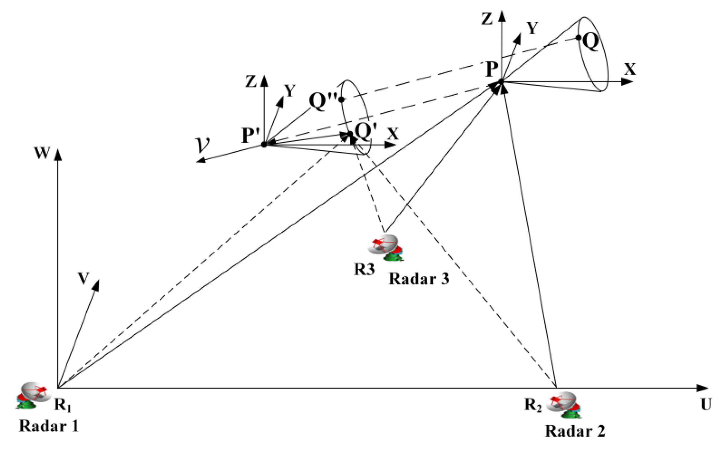
The geometry model for the radar network imaging is shown in Figure 1, where three radars will simultaneously and independently observe the target from different angles and the target is located in the far field. The observation data in the different perspectives will be fused to overcome the anisotropy problem. A local Cartesian coordinate is defined, where the origin is the location of Radar 1. The coordinate system move along with the translational motion direction and the origin is the imaging center point. The axis , , and are parallel with the axis , , and , respectively.
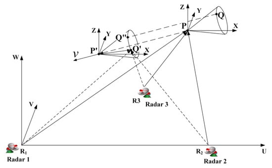
Figure 1.
The radar network imaging geometry.
Suppose the point Q is a scatterer. The vector matrix , , and denote the rotation matrix, coordinates of the scatterer, and angular velocity vector with respect to the coordinate system , respectively. The vector is defined as the velocity vector of the translational motion with respect to the coordinate system . Among them, the rotation matrix is determined by
where ,
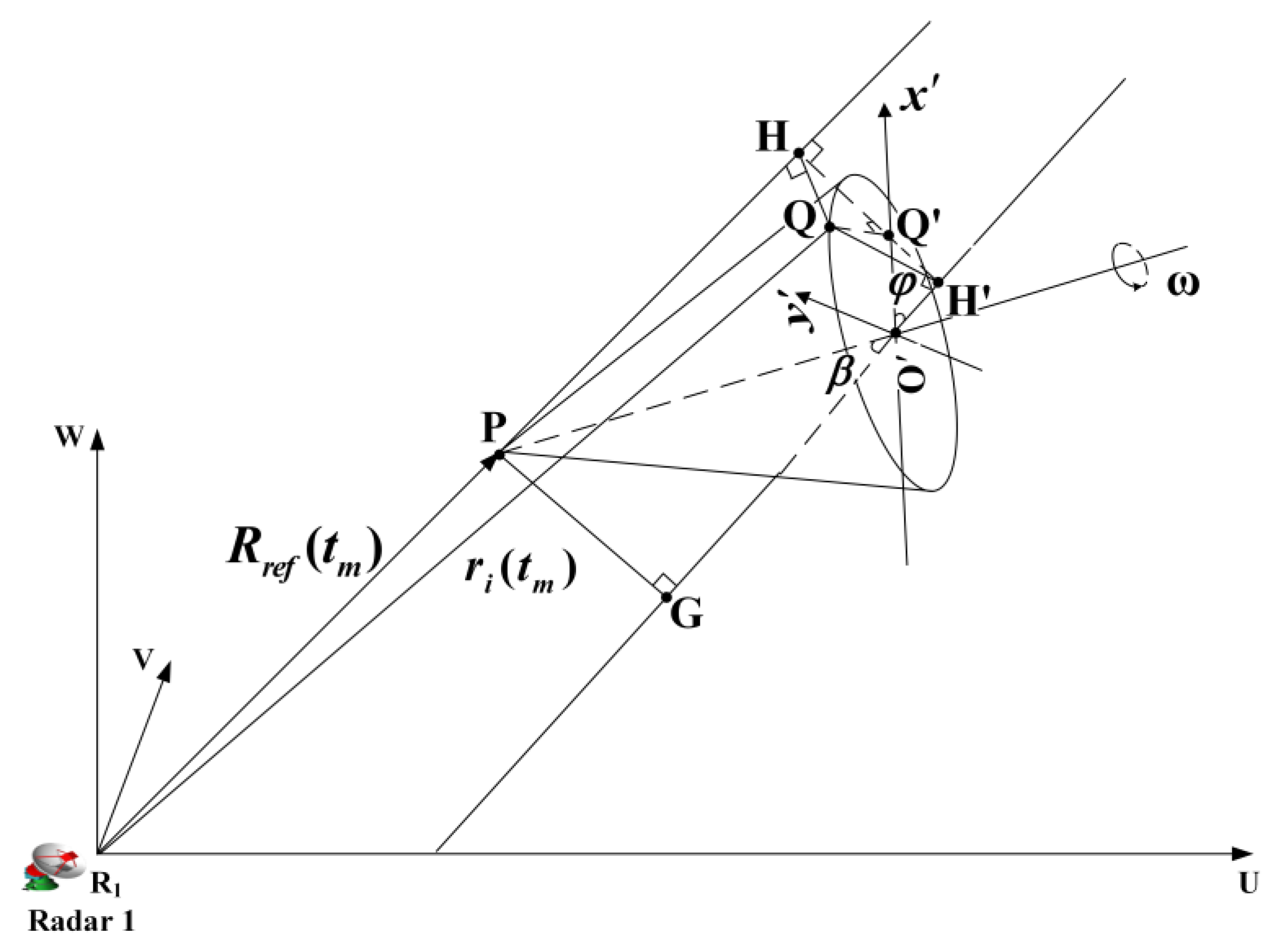
To analyze the mapping process, it is effective to analyze the 2D imaging principle. The diagram of the spinning target in the imaging scene is shown in Figure 2. The spinning scatterers incorporate the micromotion and translational motion, while the imaging center point incorporates the translational motion. Therefore, the distance between the radar and the spinning scatterer is calculated as follows:
and the distance between the radar and the imaging center point is calculated as follows:
where is the vector from the radar 1 to the imaging center point with respect to the coordinate system at the imaging initial moment. is the coordinates of the imaging center point and is the coordinates of the radar 1.
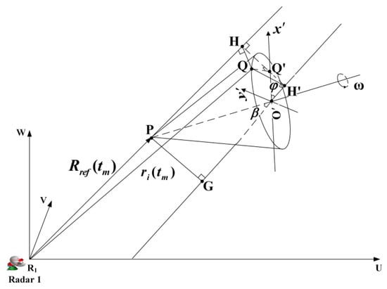
Figure 2.
The diagram of the spinning target in the imaging scene.
Support the point is the mapping of the point on the spinning plane and the line is parallel with the spinning axis. Thus, the line is perpendicular to the spinning plane and is parallel with the bulk-motion direction. The line is parallel with the line which is the extension cord of the line and the point is the intersection between the line and the line . Therefore, the plane is the imaging plane. The axis is defined as the intersection between the plane and the spinning plane, and the axis constrained on the spinning plane is perpendicular to the axis . Support the point is a scatterer and the line is perpendicular to the axis . Because the line is perpendicular to the axis and the line , respectively, the line is perpendicular to the plane and the point is the mapping of the scatterer on the imaging plane. Let the line be perpendicular to the line and the point be the intersection between the line and the axis . Because the line is perpendicular to the line and the line , the line is perpendicular to the line .
According to the geometrical relationship, the relative distance between the scatterer and the imaging center point can be calculated. The point is located on the axis , and the coordinates of the point is defined as with respect to the coordinate system . Considering that the target is located in the far field, the approximate solution of the relative distance will be determined by
where and are the constant, as shown in Figure 2. For the spinning scatterer , the coordinate is a sinusoidal function of time. Therefore, the micro-Doppler signature is a sinusoidal function of frequency due to the coordinate .
3.2. Analysis of the Mapping Process
Because the scatterer spins around and around, when the spinning scatterer is mapped onto the imaging plane is not clear. Therefore, it is necessary to deduce the mapping moment when the spinning target is mapped onto the imaging plane.
In the 2D continuous space, the Radon transform of the image over the axis at a given angle is
For the distribution function , its Radon transform can be expressed as follows:
Therefore, the Radon transform of the distribution function of a point in the domain satisfies
As usually reported, is the length of the apothem associated with the chord formed when a straight line secant to the spinning scatterer, and is the angle between the axis and the line perpendicular to the chord. For the fixed point, and are the constant, and the is a sinusoid in the domain. The inverse Radon transform of is the reconstructed distribution function .
Let a spinning point rotate clockwise around the origin of the coordinate system like the spinning scatterer, as shown in Figure 3. The coordinates of the spinning point are and the angle between the line and the axis is at the initial time. After the point spins by degree, the coordinates about the axis can be calculate as follows:
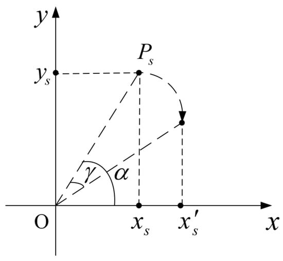
Figure 3.
The rotation geometry for the spinning point.
By contrasting (16) and (17), it is found that the variable , and the constant , are equivalent to the variable , and the constant , , respectively. By analogy, the point distribution function can be regarded as the result of the inverse Radon transform in the domain. Suppose the spinning point is a scatterer, Equation (17) should become the micro-Doppler signature of the spinning scatterer, and its micro-Doppler signature can be roughly depicted as Figure 4a. Therefore, we can infer that, by performing the inverse Radon transform to the micro-Doppler signature, it is transformed to the distribution function on the imaging plane. The distribution function indicates the coordinates of the spinning scatterer at the spinning initial time. The spinning initial time can be considered as the imaging initial time.
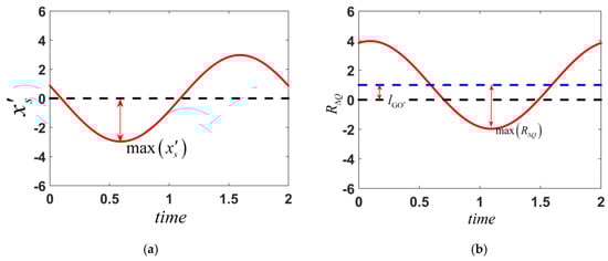
Figure 4.
The theoretical micro-Doppler signature. (a) the curve of to time. (b) the curve of to time.
Micro-Doppler signature induced by micromotion is the imaging result in range-slow time domain or frequency-slow time domain. For the spinning scatterer in the imaging scene, the amplitude of the micro-Doppler signature will vary as the variable change, as shown in (13). There is a linear relationship between the relative distance and the coordinate , thus the relation curve (i.e., micro-Doppler signature) can be roughly depicted as Figure 4b. Because the angle is determined by the initial coordinates of the scatterer in the domain, the initial phase of the micro-Doppler signature is also determined by the initial coordinates. The sinusoidal curve in the domain generated with the scatterer rotation is identical to the micro-Doppler signature (as shown in Figure 4b), where the coordinate is the linear transform of the variable like (13) and the angle is the rotation angle of the scatterer. After performing the inverse Radon transform to the sinusoidal curve in the domain, the transform results is the distribution function of the spinning scatterer in the domain and the distribution function indicates the scatterer position at the imaging initial time. Then, the distribution function of the scatterer in the domain can be obtained by performing the linear transform to the coordinate . Considering that the coordinate system is on the spinning plane, we define the 2D image plane as the spinning plane. Therefore, the 2D image obtained by the range compression and the inverse Radon transform can be regarded as the mapping of the spinning scatterer on the 2D image plane. The imaging initial time is the mapping time. After the linear transform in the domain, the mapping will be equivalent to the 2D image.
3.3. Mapping Formulas and Mapping Image
Let the vector and denote the normal vector perpendicular to the plane and the spinning plane, respectively. Among them, the vector is the cross product between the vector and , while the vector is parallels with the vector . The vector and are expressed as follows:
where , , and are the unit vector of the axis with respect to the coordinate system . Because the axis is perpendicular to the vector and , the normal vector of the axis will be calculated by the cross product operation. The normal vector of the axis is the cross product between the vector and . Thus, the vector and are expressed as follows:
The is selected as a spinning point which will be mapped onto the 2D image plane. Suppose the coordinates of the point is with respect to . Therefore, the plane which is the spinning plane of the point and is perpendicular to the vector can be expressed as follows:
where the is the coordinates of the point on the plane . Let the point be the mapping of the imaging center point on the 2D image plane. The mapping line through the imaging center point and perpendicular to the 2D image projection plane is expressed as follows:
where is the coordinates of the mapping line with respect to the real variate . The mapping of the imaging center point is the intersection of the plane and the mapping line. Substitute the formula of the mapping line into the formula of the plane , we can gain the expression as follows:
Equation (24) can be written as:
The coordinates of the point with respect to will be calculated as follows:
Depending on the normal vector , , and the coordinates , the coordinate system is built on the 2D image plane.
The coordinates of the point in the domain can be calculated by
where the vector is . As shown in Figure 2, the constant and can be calculated as follows:
Therefore, after the linear transform, the coordinates of the point in the domain can be calculated as follows:
So far, the formulas for mapping the spinning point onto the 2D image plane are presented. As mentioned above, the proposed method makes use of the similarity of the imaging result with the mapping on the 2D image plane to reconstruct the target 3D image. The air point whose mapping on the 2D image plane coincides with the reconstructed point in the 2D imaging result could be a scatterer and its position in 3D Cartesian space would contain a scatterer. Taking the imaging result minus the mapping image of the air point is a way to determine the scatterer distribution. Therefore, it needs to form the mapping image which has the same resolution unit with the 2D imaging result. The mapping image can be achieved by using the mapping coordinates of the air points.
Let denote the range resolution and signify the sampling numbers on the range direction. Thus, the length of the range bin in the 2D image is the and the sampling numbers of the 2D image on the range direction is . The plane grid for the mapping image, which is same as the grid of the imaging result, is depicted in Figure 5. Every grid unit may be occupied by the mapping point.
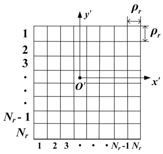
Figure 5.
The plane grid for the mapping image.
For the imaging center point, its mapping point is . The serial number of the grid occupied by the point in the direction of the axis and axis are and , respectively. Therefore, the grid serial number with respect to the mapping of the point is determined by
where the mathematical symbol is the rounding-off method. Therefore, the mapping image is achieved by calculating the serial number about the mapping point and filling the corresponding grid unit. To measure the similarity of two images, we can calculate the minus value between the imaging result and the mapping image. In this way, the scattering distribution would be confirmed.
4. 3D Image Reconstruction for Spinning Target
In this section, the reconstruction method for the 3D image of the spinning target is proposed based on the radar network. The radar network is constituted by the distributed radars and each radar observes the target independently from different perspective. According to the anisotropy, the available scattering information for each radar would normally be incomplete due to the limited observation perspective, even though the monostatic radar may observe the air target for a long time. Therefore, each radar would provide partial observation information about the target and all the observation information should be fused to form the 3D image. In this paper, a reconstruction method for the scattering distribution is proposed based on the monostatic radar, but the scattering distribution is incomplete due to the anisotropy. Then, by fusing all the scattering distribution, the 3D image of the spinning target will be reconstructed.
4.1. Scattering Distribution Reconstruction Based on the Monostatic Radar
To generate the mapping image, it needs to map the air points onto the 2D image plane. In the process, the target area is transformed into a grid area to simplify the air point number. The grid area is defined as the cube which is large enough to contain all the target scatterers, as shown in Figure 6. All the scatterers are in the grid cell of the grid area. Because the resolution to recognize the flight target is less than 0.3m as reported, the grid cell could be defined as a cube whose length is 0.25 m on a side. When the mapping of the grid cells onto the 2D image plane coincides with the 2D imaging result, these cells among the grid area are considered as the potential cells where the scatterers locate with high probability. Therefore, it is feasible to construct the scattering distribution of the spinning target by searching out the scatterers from the grid area.

Figure 6.
The air grid area. The target 3D model is constituted by the black points which are considered as the target scatterers. All the scatterers are in the cell.
However, not all the potential cells contain the scatterers, because the point on the plane parallel to the target’s bottom may have the same mapping as the scatterers. Therefore, for reconstructing the 3D image of the spinning target, it is necessary to determine which plane is the target’s bottom and which cells on the plane contain the scatterers.
It is well known some target characteristics can be obtained from the micro-Doppler signatures, thus the micro-Doppler signatures may provide the micro-Doppler feature about the target’s bottom. Substitute the (13) into the (3), the micro-Doppler signature in the time-frequency domain can be expressed as
The time-frequency micro-Doppler signature is the sinc function and is also the range profiles of the scatterers. The frequency value of the micro-Doppler signature is determined by the sum of the second and third terms of the sinc function where the second term is a sinusoid with respect to the time and the third term is a constant. Therefore, for the micro-Doppler signature, the amplitude of the sinusoid is influenced by the second term of the sinc function and the offset distance of the sinusoid in the frequency domain is determined by the third term. The sinusoid and the offset distance in the frequency domain are shown in Figure 7.
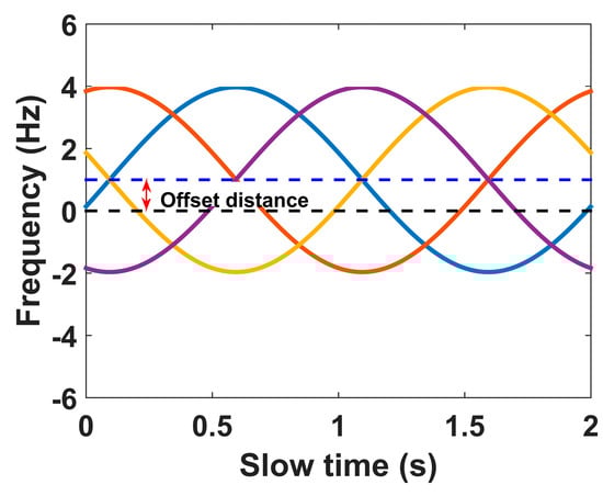
Figure 7.
Time-frequency micro-Doppler signature. The blue line is zero frequency line and the black dotted line is the line whose frequency is equal to the offset distance.
Because the coordinates of the imaging center point P and the normal vector are known, the target’s bottom can be confirmed by calculating the length of the line . As shown in Figure 2, the length of the line can calculated by the length and the angle according to the law of Sines. The angle is calculated as follows:
Because the offset distance , the length can be calculated after the offset distance is obtained. The EHT is a method for sinusoid detection and four-parameter estimation by mapping the sinusoid to a four-parameter space [33]. The four parameters include the angle frequency, initial phase, maximum extent, and offset distance of the sinusoid. Therefore, the offset distance can be calculated by the EHT and the mapped sinusoid is the micro-Doppler signature.
As mentioned above, the imaging result is identical to the mapping image, thus we attempt to reconstruct the scattering distribution of the spinning target by using the principle. The scattering distribution reconstruction model based on the monostatic radar for the spinning target can be determined by
where the three-dimensional matrix representing the grid area matrix contains only 0 or 1. The element 1 in the matrix , such as , indicates that the cell contains a scatterer. The matrix set expresses the search scope of the matrix and the matrix set expresses a part of the matrix set . For the matrix set , the cells whose offset distance of the micro-Doppler signature are unequal to contain no scatterer. Thus, the elements corresponding to these cells in the matrix are always 0, and other elements may be 0 or 1. For the m-th radar in the radar network, the function is the mapping formulas and the two-dimensional matrix is the 2D image obtained by the range compression and inverse Radon transform. The goal of the model is to minimize the reconstruction error.
The proposed algorithm for solving the scatterering distribution reconstruction model is depicted in Algorithm 1. Let the optimum matrix be denoted by , and let be the cell number on the side of the cubic grid area.
| Algorithm 1. A reconstruction algorithm for solving the scattering distribution reconstruction model. |
| Algorithm for (37) |
| 1. Define the set as the serial number of cells of the grid area; 2. Obtain the 2D image with respect to the m-th radar by the range compression and inverse Radon transform; 3. Extract the micro-Doppler signature about every reconstructed point in the 2D image by the Radon transform; Obtain the offset distance by the EHT and calculate the length ; Set and the set of the cells which are on the spinning plane is ; 4. For Set is the serial number of the cell and its coordinates are with respect to the coordinate system ; Calculate the distance between the imaging center point and the i-the cell, i.e., ; Calculate the distance from the imaging center point to the spinning plane of the i-the cell, i.e., ; Define the mapping of the imaging center point on the spinning plane of the i-the cell is ; According to the distance and the angle , the length can be calculated by ; If ; end end ; 5. Set is the number of the elements in the set ; For Set ; Calculate the mapping according to the mapping formulas; ; If ; end Set ; end 6. Set is the number of the elements in the set ; For ; end The optimum matrix ; 7. end. |
For the situation that the scatterers are not on the same spinning plane, the reconstruction algorithm also applies to the scattering distribution reconstruction model. For two scatterers which have different spinning plane, their micro-Doppler signatures have different offset distance. After performing the Radon transform to every reconstructed point in the 2D image, the micro-Doppler signature about every point is extracted and its offset distance can be calculated by the EHT. The different spinning plane can be distinguished by the different offset distance. For the different spinning planes (i.e., the different length ), their scattering distribution can be obtained by using the reconstruction algorithm, respectively. All the scattering distribution which is observed by the individual radar in the network would constitute the intact scattering distribution about the spinning target.
4.2. 3D Image Reconstruction Based on the Radar Network
In the process of reconstructing the 3D image of the spinning target, we wish that every radar in the radar network has the minimal error between its imaging result and its mapping image. In addition, the reconstructed 3D image should not be constituted by superabundant scatterers. To minimize the error and control the number of the reconstructed scatterers, the 3D image reconstruction model for the spinning target based on the radar network is determined by
The parameter is the weight coefficient of the reconstructed scatterer number. In contrast to the scattering distribution reconstruction model in (37), the 3D image reconstruction model can be considered as the superposition of all scattering distribution reconstruction models. Every radar will obtain a scattering distribution which is affected by its observation perspective. Because every scattering distribution reconstruction model has linear relation with the others in the 3D image reconstruction model and they have no tight coupling, every reconstructed matrix is mutually independent. The 3D image of the spinning target can be generated by adding up all the scattering distribution (i.e., all the reconstructed matrix).
The concrete steps of the 3D image reconstruction for the spinning target based on radar network are as follows:
- Obtain the ISAR imaging results with respect to every radar by the range compression and inverse Radon transform.
- Extract the reconstructed points in the imaging results (i.e., the peaks in the images), and perform the Radon transform to every reconstructed point to obtain its micro-Doppler signature.
- Calculate the offset distance of every micro-Doppler signature by the EHT.
- Determine the mapping formulas for every radar by (18)~(34).
- Reconstruct the scattering distribution on every spinning plane by the scattering distribution reconstruction method. When the scattering distribution about every radar is obtained, go to step 6.
- Reconstruct the 3D image of the spinning target by adding up all the scattering distribution.
4.3. Error Analysis
As shown in the algorithm flow, the main steps for reconstructing the 3D image contain ISAR imaging, the mapping image generation, and 3D image reconstruction. Because of the resolution in ISAR imaging, the resolution of the mapping image must be equal to . Therefore, in the mapping process, the mapping result would exist the mapping error in the direction of the axis and the axis , and the mapping error range is in the domain. In addition, in the process of calculating the offset distance by the EHT, the distance error would result in the part of the reconstruction error in the direction perpendicular to the spinning plane. For any two points, suppose the and are the distance from the imaging center point to the spinning plane of the points, respectively. Let the and are the coordinates in the corresponding axis, respectively. When the inequality (39) is met, the two points have the same mapping position in the mapping image. Thus, suppose one of the points is a scatterer, then the two points are all likely to be considered as the scatterer.
Inequality (39) can be rewritten as:
Equation (40) is also the error range of the mapping image in the direction of the axis, and we can see that the range of (i.e., the error range) is always regardless of . Therefore, the maximum of the reconstruction error is in the direction of the axis, then the resolution in this direction can be considered as . Because as shown in (32), the error range in the direction of the axis is , and the resolution in the direction is .
5. Results
In this section, we contrast the imaging results with the mapping images of the target model to verify the validity of the mapping formulas firstly. After extracting the micro-Doppler curves and calculating the offset distance, the scattering distribution for every radar is reconstructed and the 3D image reconstruction is accomplished by fusing all the scattering distributions.
5.1. Comparison between the Imaging Result and the Mapping Image of the Target Model
The radar network is composed of three imaging radars which are located at km, km, and km, respectively. All the radars have the same configuration. The radar bandwidth is 300 MHz, the range resolution is 0.5 m, and the radar pulse repeated frequency (PRF) is 1000 Hz. The position of the imaging center point is km at the initial moment, the velocity vector is m/s, and the angular velocity vector is rad/s.
The radar distribution is shown in Figure 8 and the spinning target consisting of 9 ideal scatterers is shown in Figure 9. In Figure 8 and Figure 9, the units are in kilometers. To verify the mapping formulas, the mapping images of the target model are compared with the imaging results. The comparison results are illustrated in Figure 10. In this experiment process, the target containing more scatterers would make it more convincing, thus the anisotropy problem may not be considered in this part. Three radars image the target from the different perspectives independently and simultaneously. The time to calculate the mapping image must be consistent with the imaging initial time. The imaging results are illustrated in Figure 10a,c,e and the mapping images are illustrated in Figure 10b,d,f. We can see that the mapping image of the spinning target are identical with the 2D imaging results, thus the veracity of the mapping operation and formulas are verified.

Figure 8.
Radar distribution. The units are in kilometers. The red, green, and blue square represent Radar 1, Radar 2, and Radar 3, respectively.

Figure 9.
Spinning target model. The units are in kilometers.
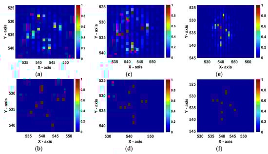
Figure 10.
The comparison between the 2D imaging results and the mapping image. (a,c,e) are the imaging results obtained by Radar 1, 2, and 3, respectively. (b,d,f) are the mapping image with respect to Radar 1, 2, and 3, respectively.
5.2. 3D Image Reconstruction
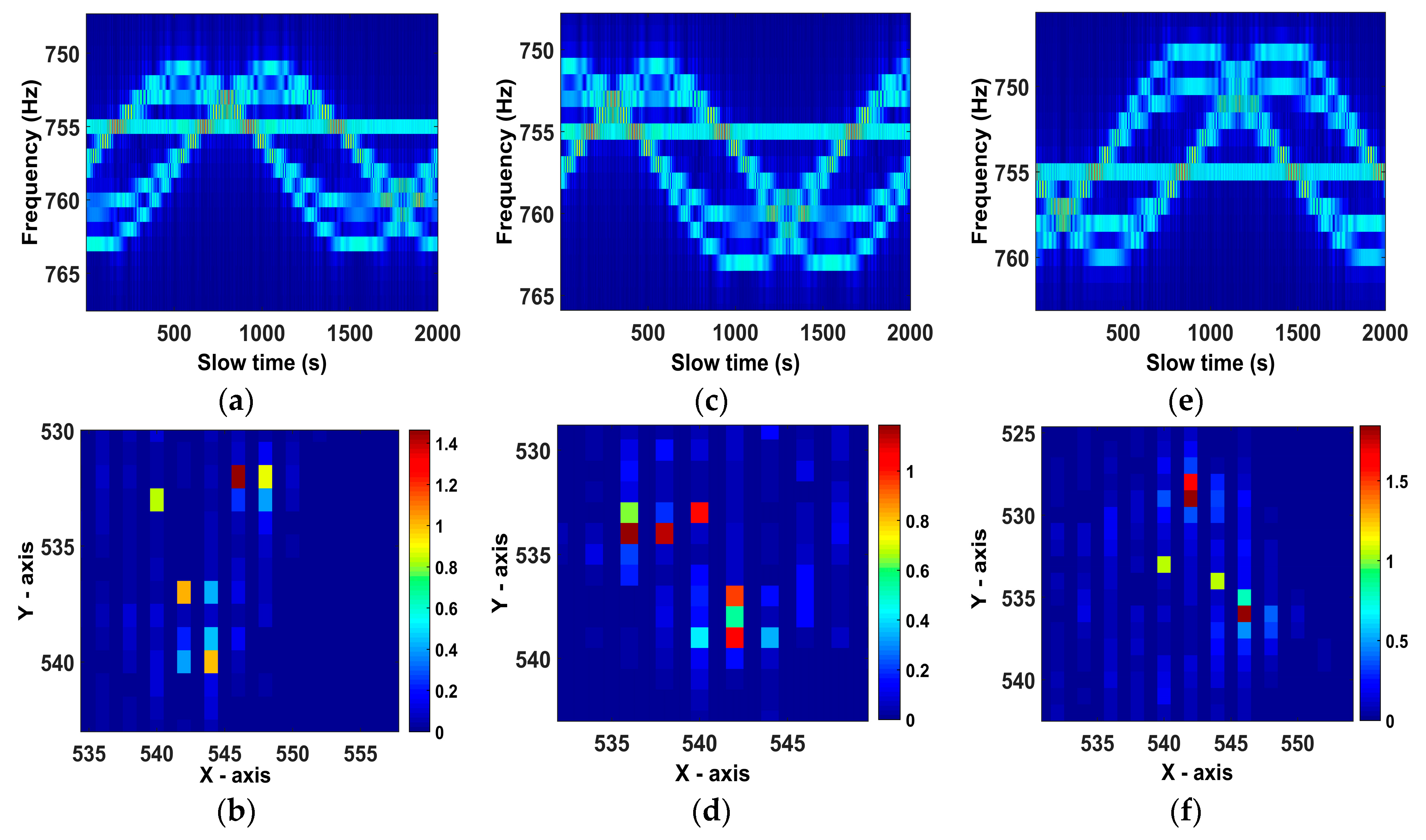
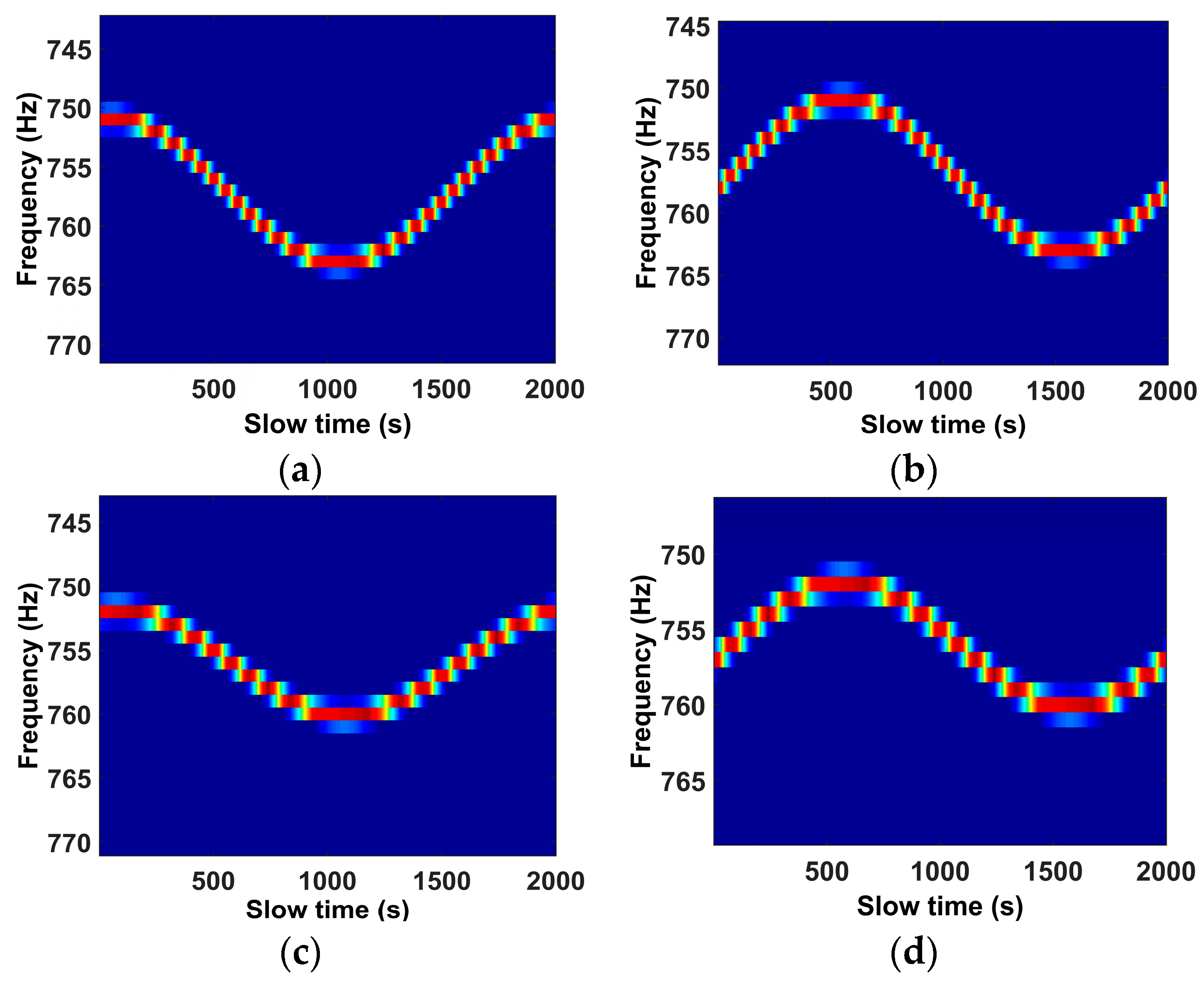
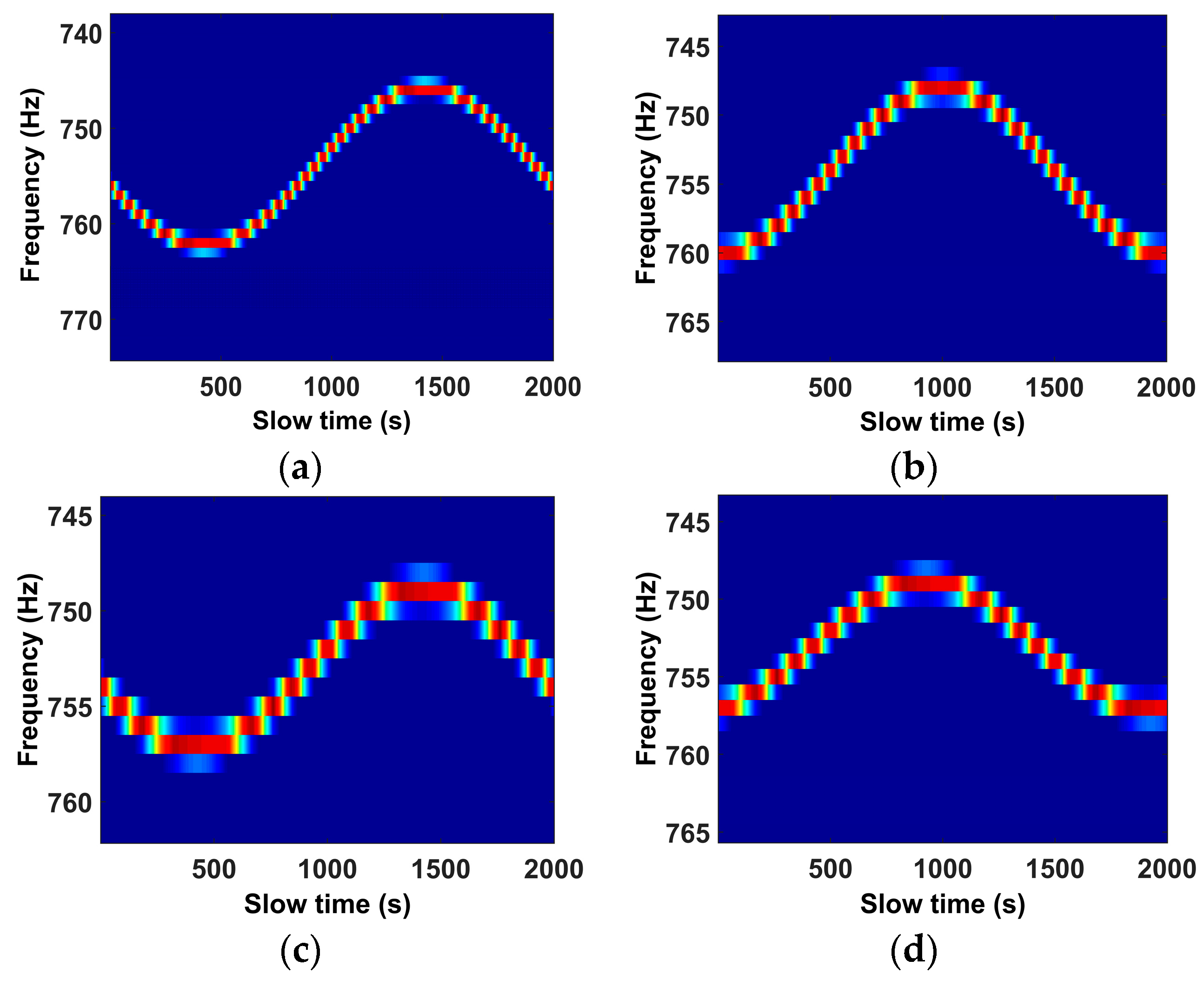
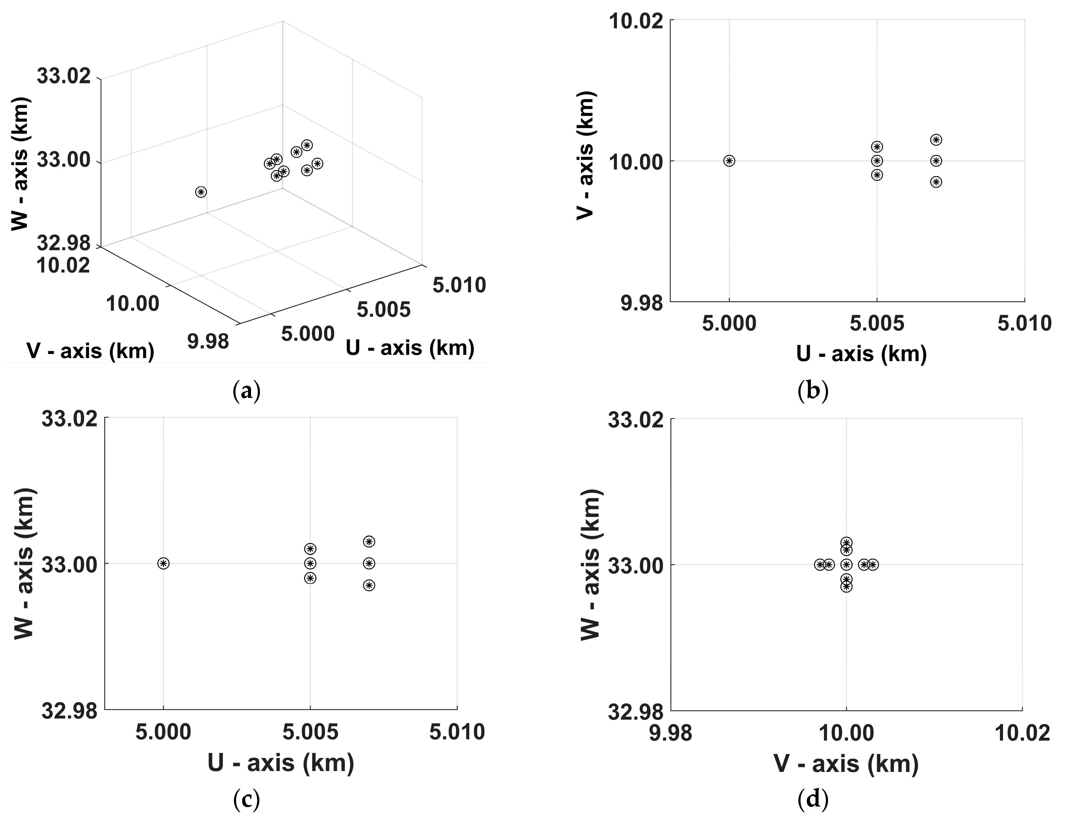
Due to the anisotropy problem, any one of the radars cannot observe all the scatterers, thus we pin our hope on the radar network which can observe the target from the different perspectives and may observe all the scatterers. For the ideal scatterer model, we preset the scattering distribution for every radar according to the relative position of the target and the radar, and the radar can only observe partial target scatterers. For every radar, the scattering distribution they can observe is illustrated in Figure 11. Radars image the target independently and the micro-Doppler signatures obtained via the range compression are shown in Figure 12a,c,e. After performing the inverse Radon transform to the micro-Doppler signatures, the imaging results are shown in Figure 12b,d,f. The extend Hough transform has better performance when there is only one sinusoid curve. Therefore, to calculate the offset distance exactly, we extract the reconstructed points in the imaging results (i.e., the peaks in the images), respectively. After that, for every reconstructed point, its micro-Doppler signature is reconstructed by the Radon transform as shown in Figure 13, Figure 14 and Figure 15. The offset distance of the micro-Doppler signature about the reconstructed point in the 2D image can be calculated by the extended Hough transform. The offset distance parameters obtained via the extended Hough transform are illustrated in Table 1. Taking advantage of the 2D imaging results, the imaging moment, and the offset distance parameter, the scattering distribution about every radar can be reconstructed by the scattering distribution reconstruction method. The reconstruction results are shown in Figure 16. The 3D image of the spinning target based on the radar network is obtained by fusing all the scattering distribution. The simulation results are shown in Figure 17. It has proven that the proposed method is efficient to reconstruct the 3D image of the spinning target in the radar network.

Figure 11.
Scattering distribution. (a–c) are the observable scattering distribution from Radar 1, Radar 2, and Radar 3, respectively.
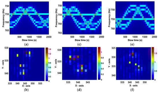
Figure 12.
Micro-Doppler signature and 2D imaging results obtained by the radars. (a,b) are the results obtained by Radar 1. (c,d) are the results obtained by Radar 2. (e,f) are the results obtained by Radar 3.
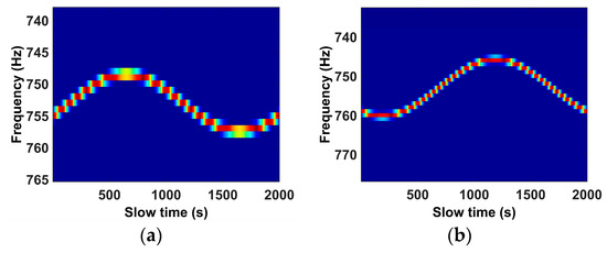

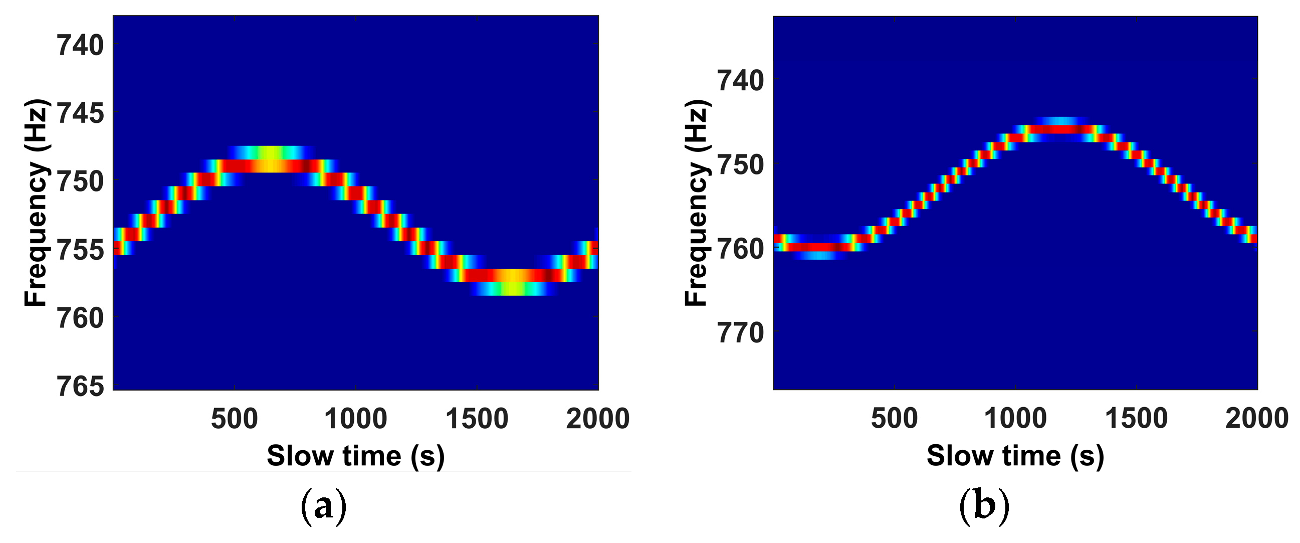
Figure 13.
The micro-Doppler signatures are reconstructed by the Radon transform. (a–d) represent the micro-Doppler signature with respect to one of the reconstructed scatterers in Figure 12b.
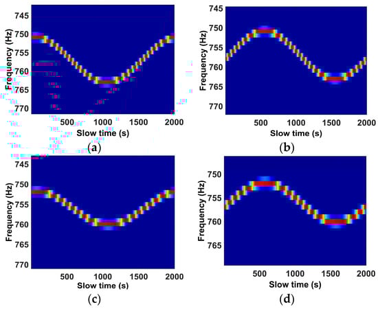
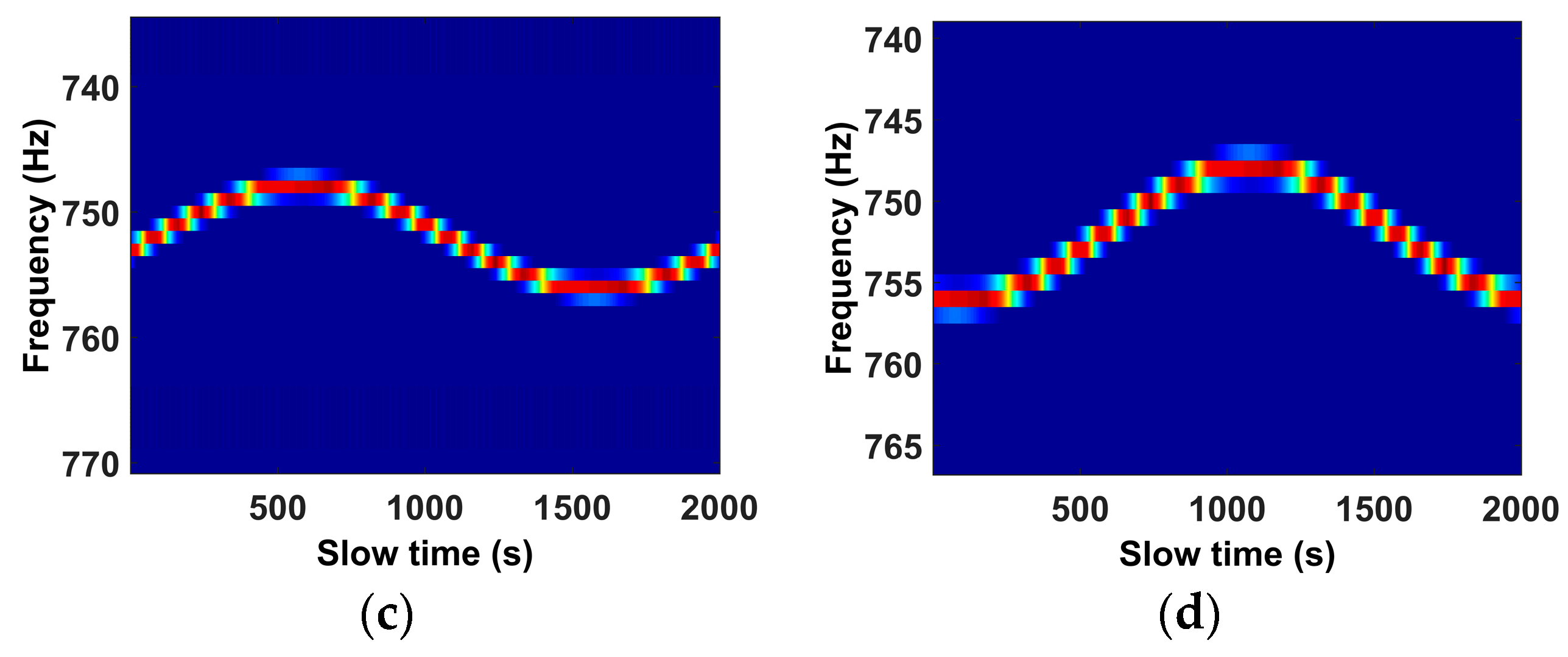
Figure 14.
The micro-Doppler signatures are reconstructed by the Radon transform. (a–d) represent the micro-Doppler signature with respect to one of the reconstructed scatterers in Figure 12d.
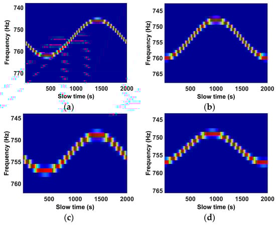
Figure 15.
The micro-Doppler signatures are reconstructed by the Radon transform. (a–d) represent the micro-Doppler signature with respect to one of the reconstructed scatterers in Figure 12f.

Table 1.
The Offset Distance.
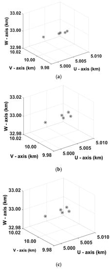
Figure 16.
Scattering distribution reconstruction results. The units are in kilometers. (a–c) are the reconstruction results obtained by Radar 1, Radar 2, and Radar 3, respectively. The asterisks and the circles represent the target model and the reconstructed scattering distribution, respectively.

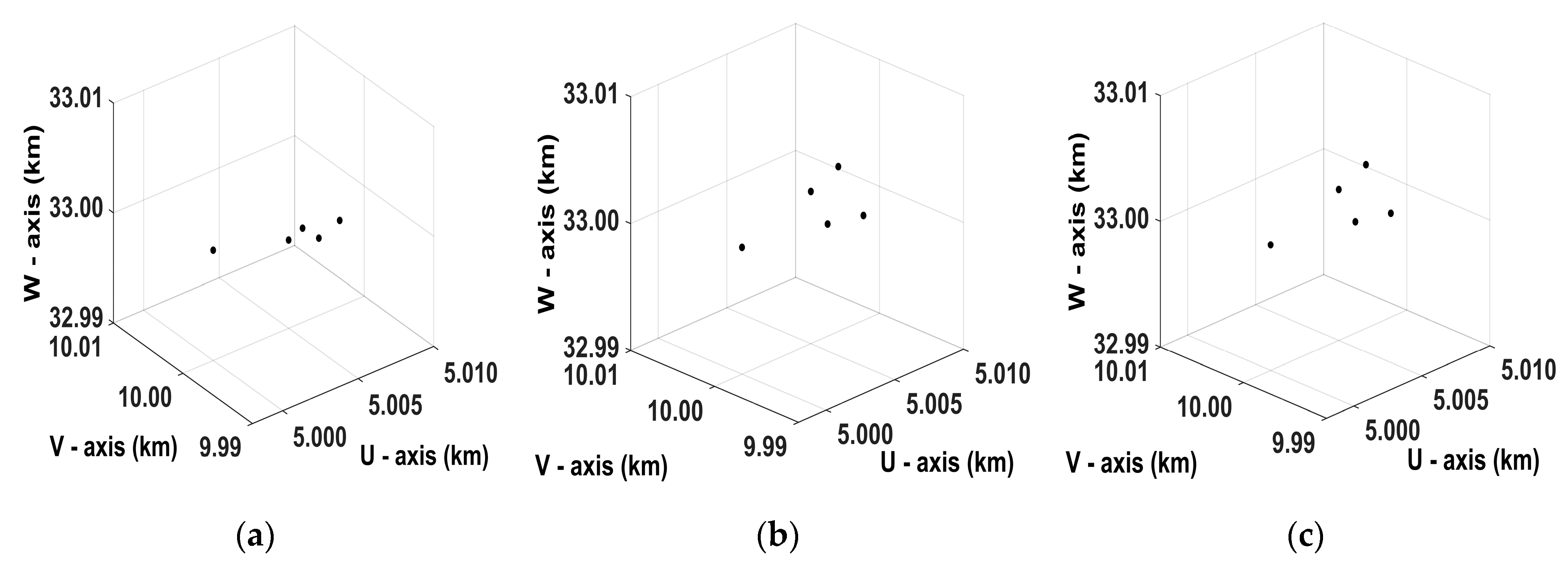
Figure 17.
3D image reconstruction result of the spinning target and its three different views. The units are in kilometers. (a) The reconstructed 3D ISAR image. (b) The reconstructed 3D ISAR image in the plane U-V. (c) The reconstructed 3D ISAR image in the plane U-W. (d) The reconstructed 3D ISAR image in the plane V-W. The asterisks and the circles represent the target model and the reconstructed scattering distribution, respectively.
To evaluate the performance of the proposed algorithm quantitatively, the mean square error (MSE) of the recovered 3D target geometry is calculated in the terms of Euler distance error. For each signal-to-noise ratio (SNR), 500 different noise realizations are used to calculate the average MSE. The imaging performance of the proposed method is compared with the interferometric 3D imaging method in different SNR (as shown in Figure 18a). Unlike the interferometric 3D imaging method which will be affected when the noise is overwhelming, the MSE of the reconstructed scatterers obtained by the proposed method is small (as shown in Figure 18). Thus, the proposed algorithm has very good robustness to noise. Practically, the 2D ISAR imaging method can get rid of much noise so that the 2D imaging result is almost unaffected by noise.
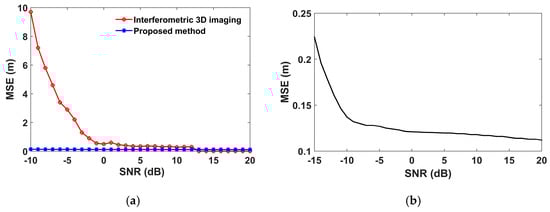
Figure 18.
The reconstruction MSE with respect to SNR. (a) The comparison of MSE between the proposed method and interferometric 3D imaging. (b) The MSE of the reconstructed scatterers obtained by the proposed method.
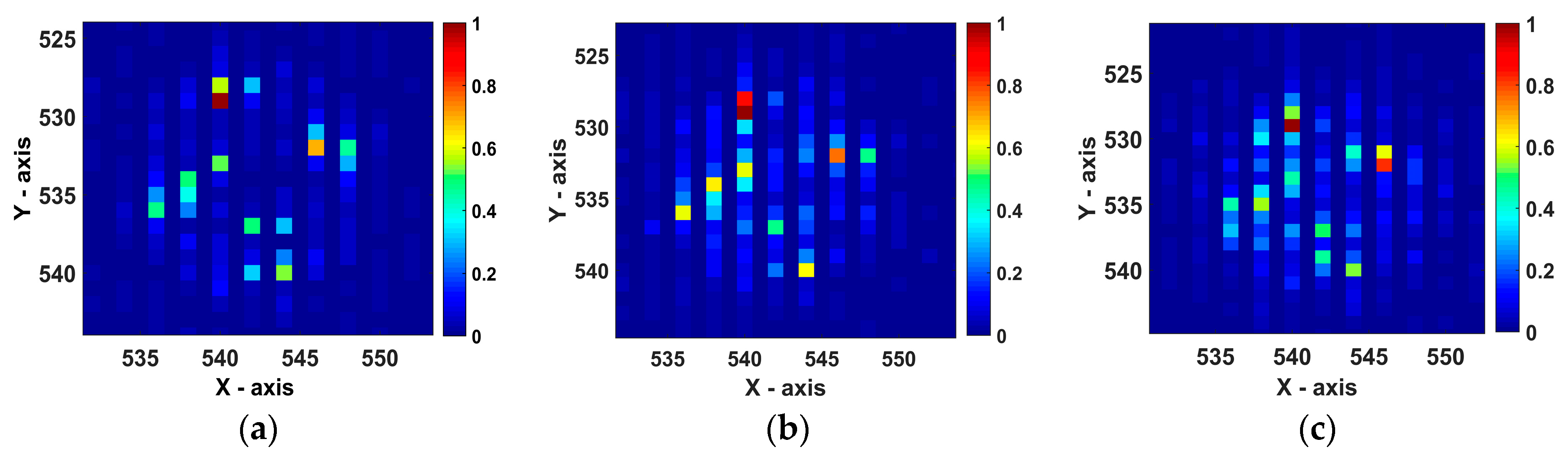
The spinning scatterer with the steady angular velocity has sinusoidal modulus and phase in the range-slow time domain, thus its micro-Doppler signature which is a sine function can be transformed into the distribution function of the spinning scatterer by the inverse Radon transform. When the inverse Radon transform is used to calculate the 2D image, the angular velocity, strictly speaking, should be a constant and could not change. The situation that the angular velocity changes slightly is analyzed by the simulation experiments to the imaging performance, and the results are as shown in Figure 19.
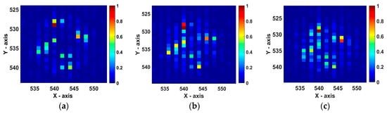
Figure 19.
The 2D imaging results of the target with different variation in angular velocity and they are obtained by Radar 1. (a) The angular velocity is constant. (b) The angular velocity changes ten degrees per second. (c) The angular velocity changes twenty degrees per second.
It can be seen that the 2D imaging method can produce the image with lesser error when the angular velocity changes ten degrees per second, thus 3D image with less reconstruction error can be obtained. While the angular velocity changes twenty degrees per second, the 2D image (i.e., Figure 19c) exists obvious different compared to Figure 19a. We roughly estimate that the 2D imaging result starts to deteriorate when the angular velocity changes more than ten degrees per second. The lower-quality 2D image will severely degrade performance of the 3D image reconstruction.
6. Discussion
The greatest strength of the proposed method is to prove a method for the radar network to reconstruct the 3D image of the spinning target, and the anisotropy problem which is caused when the radars in the network observe the target from the different perspectives is overcome in the proposed method. At present, interferometric technique is regarded as an effective method to reconstruct the 3D image with high precision, and there are several novel and cutting-edge papers [10,11,14,20,30] which study the interferometric technique to reconstruct the 3D target image. In the interferometric 3D imaging method, L-shaped three-antenna configuration or the Bistatic radar configuration is necessary to generate the interferometric signal and calculate the interferometric phase. However, how to reconstruct 3D target image by the radar network which is constituted by several independent imaging radars is relatively unexplored. Because the radar network possesses high flexibility in the radar configuration, it has the potential to improve the 3D imaging quality and overcome the existing problems in the process of the 3D imaging.
The main problem of the interferometric 3D imaging technique is the robustness to noise. Because the noise affects the interferometric phase, the interferometric results in position will generate deviation from the real value. Therefore, the performance of the interferometric 3D imaging method is always affected when the noise is overwhelming. As reported in the paper [12], when SNR is higher than 3 dB, MSE holds a steady trend which is less than about 0.3 m, and the interferometric 3D imaging method can achieve satisfactory results. By contrast, the 3D image reconstruction method proposed in this paper has a better robustness to noise, as shown in Figure 18. When SNR is at the level of −15 to 20 dB, the MSE of the reconstructed scatterers obtained by the proposed method is small. For the proposed method, the primary task is to obtain the 2D imaging result of the spinning target and the mapping of the air points. The 2D imaging method depending on the range compression can get rid of much noise, while the mapping process does not involve noise. Therefore, the reconstructed 3D image result obtained by the proposed method is less affected by noise.
Although the reconstruction error does not appear to be easily seen in the reconstructed 3D image, as shown in Results, the reconstruction error is virtually existent as recited in Error analysis. The mainly reason of the error produced is the gridding air area and the gridding imaging plane. This kind of error can also be considered as the reconstruction resolution. There is another aspect to the error produced: the calculation error, such as calculating the offset distance by the EHT, would lead to the reconstruction error. However, as shown in the simulation experiment, the reconstruction error could be small when selecting the appropriate air grid size, i.e., the appropriate resolution.
The proposed 3D image reconstruction method can overcome the anisotropy problem and the strong noise and is appropriate for the target with slightly variational angular velocity, however, it is evident that the full potential of radar network to reconstruct the spinning target 3D image has not yet been explored. A few research priorities and recommendations on the way ahead emerge from this review:
- As shown in the experiments, when the angular velocity changes roughly more than ten percent per second, the 2D imaging result starts to deteriorate and it can severely degrade performance of the 3D image reconstruction. Although the angular velocity is often considered as a constant in current research, it is also significant to study the 3D image reconstruction for the target with variational angular velocity. We urge future research to focus on the 2D and 3D imaging for the spinning target with variational angular velocity.
- The radars in network are required to observe the target from different angles simultaneously and independently. In other words, we must use the observation data obtained by the different radars in the same period. It obviously lacks the flexibility in the multi-radar observation. If we can propose a radar network 3D imaging method which can adopt a flexibility observation mode, it would have the potential to obtain a better 3D imaging result.
- The optimal deployment problem of the radar network is an important research content in space target surveillance and imaging task. Future research must be focused on the optimal deployment problem of the radars to improve the performance of the 3D image reconstruction and the use of the radar resources.
- There is not real radar data we can use in the experiments of the 3D image reconstruction for spinning target in radar network. On the one hand, now we indeed have no ability to set up a real radar network experimental platform for the space target 3D image reconstruction problem. On the other hand, there is bare minimum of available real radar data acquired by the radar network in the field of the space target imaging research currently, especially the space spinning target 3D imaging research. In current work [13,14,15], the simulation data is usually used to verify the space target imaging method. Future work must be focused on constructing the real radar network experimental platform and verifying the proposed method in using real radar data.
With the increasing numbers of the space targets and the enhancement of the interference in the electromagnetic environment, it is difficult for the monostatic radar to complete all the reconnaissance and surveillance tasks. Radar technique will surely move toward networked and intelligent. Aimed at the networked direction, the proposed method in the paper has the potential to complete the 3D imaging task for the air targets in future networked radar mode. In addition, the paper also has the potential to be used in noise condition due to good robustness to noise.
7. Conclusions
In this paper, a novel 3D image reconstruction method for the spinning target based on the radar network is proposed. The radar network composed of three dispersed imaging radars in the simulation experiments can observe the target from the different perspectives and the anisotropy problem can be overcome by fusing the observation information from the different perspectives. At first, the range compression and inverse Radon transform is applied to form 2D image of the spinning target. Secondly, the process of mapping the spinning scatterers onto the imaging plane is analyzed and the mapping formulas to form the mapping image are derived. After the parameter (i.e., the offset distance) in the micro-Doppler signature is calculated, the 3D scattering distribution reconstruction model based on the monostatic radar and 3D image reconstruction model based on the radar network are constructed, respectively. Afterwards, the algorithm for solving the scattering distribution reconstruction model is proposed and the concrete steps of the 3D image reconstruction are given. The 3D image of the spinning target is reconstructed by adding up all the scattering distribution observed from the different perspectives, thus the anisotropy problem is overcome. Finally, the reconstruction error and the resolution are analyzed, and the experimental results are presented to verify that the mapping formulas and 3D image reconstruction method proposed in this paper are valid. In addition, the reconstruction MSE with respect to SNR is presented. The MSE relatively holds a steady trend when the SNR is higher than −10 dB, while the curve of MSE steeply rise when the SNR is lower than −10 dB. However, when SNR is at the level of −15 dB, the MSE of the recovered 3D target is less than 0.25 which is not enormous. In conclusion, the main contribution of this paper in the field of the 3D imaging is that it provides a 3D image reconstruction method for the radar network system to image the spinning target and provides a novel 3D image reconstruction method by taking advantage of the similarity of the imaging result with the mapping image. The mapping process is analyzed, and the mapping formulas are derived. The 3D image reconstruction model is constructed and the algorithm for the reconstruction model is proposed. Finally, the steps of the proposed method are given.
Author Contributions
X.-w.L. and Q.Z. proposed the method and designed the experiments; X.-w.L., L.J. and J.L. coordinated reading, analysing and categorizing the articles reviewed in this stud; X.-w.L. and Y.-j.C. analyzed the data; X.-w.L. performed the experiments, wrote and revised the paper.
Funding
This research and APC was funded by the National Natural Science Foundation of China grant number 61631019.
Acknowledgments
The authors would like to thank the handing editor and the anonymous reviewers for their valuable comments and suggestions for this paper. This work was supported in part by the National Natural Science Foundation of China under Grant 61631019.
Conflicts of Interest
The authors declare no conflict of interest.
References
- Joshi, N.; Baumann, M.; Ehammer, A.; Rasmus, F. A Review of the Application of Optical and Radar Remote Sensing Data Fusion to Land Use Mapping and Monitoring. Remote Sens. 2016, 8, 70. [Google Scholar] [CrossRef]
- Chen, Y.C.; Li, G.; Zhang, Q.; Sun, J. Refocusing of Moving Targets in SAR Images via Parametric Sparse Representation. Remote Sens. 2017, 8, 795. [Google Scholar] [CrossRef]
- Sadjadi, F.A. New experiments in inverse synthetic aperture radar image exploitation for maritime surveillance. In Proceedings of the SPIE—The International Society for Optical Engineering, Baltimore, MD, USA, 1 July 2014; p. 909009. [Google Scholar]
- Wang, Y.; Kang, J.; Jiang, Y.C. ISAR Imaging of Maneuvering Target Based on the Local Polynomial Wigner Distribution and Integrated High-Order Ambiguity Function for Cubic Phase Signal Model. IEEE J. Sel. Top. Appl. Earth Observ. Remote Sens. 2017, 7, 2971–2991. [Google Scholar] [CrossRef]
- Wang, Z.S.; Yang, W.; Chen, Z.M.; Zhao, Z.Q.; Hu, H.Q.; Qi, C.H. A Novel Adaptive Joint Time Frequency Algorithm by the Neural Network for the ISAR Rotational Compensation. Remote Sens. 2018, 10, 334. [Google Scholar] [CrossRef]
- Hu, X.W.; Tong, N.N.; Zhang, Y.S.; Hu, G.P.; He, X.Y. Multiple-input–multiple-output radar super-resolution three-dimensional imaging based on a dimension-reduction compressive sensing. IET Radar Sonar Navig. 2016, 10, 757–764. [Google Scholar] [CrossRef]
- Zhao, J.; Zhang, M.; Wang, X.; Cai, Z.H.; Nie, D. Three-dimensional super resolution ISAR imaging based on 2D unitary ESPRIT scattering centre extraction technique. IET Radar Sonar Navig. 2017, 11, 98–106. [Google Scholar] [CrossRef]
- Suwa, K.; Wakayama, T.; Iwamoto, M. Three-Dimensional Target Geometry and Target Motion Estimation Method Using Multistatic ISAR Movies and Its Performance. IEEE Trans. Geosci. Remote Sens. 2011, 49, 2361–2373. [Google Scholar] [CrossRef]
- Ding, S.S.; Tong, N.N.; Zhang, Y.S.; Hu, X.W. Super-resolution 3D imaging in MIMO radar using spectrum estimation theory. IET Radar Sonar Navig. 2017, 11, 304–312. [Google Scholar] [CrossRef]
- Xu, G.; Xing, M.D.; Xia, X.G.; Zhang, L.; Chen, Q.Q. 3D Geometry and Motion Estimations of Maneuvering Targets for Interferometric ISAR with Sparse Aperture. IEEE Trans. Image Process. 2016, 25, 2005–2020. [Google Scholar] [CrossRef]
- Martorella, M.; Stagliano, D.; Salvetti, F.; Battisti, N. 3D interferometric ISAR imaging of noncooperative targets. IEEE Trans. Aerosp. Electron. Syst. 2014, 50, 3102–3114. [Google Scholar] [CrossRef]
- Bai, X.R.; Bao, Z. High-Resolution 3D Imaging of Precession Cone-Shaped Targets. IEEE Trans. Antennas Propag. 2014, 62, 4209–4219. [Google Scholar] [CrossRef]
- Bai, X.R.; Zhou, F.; Bao, Z. High-Resolution Three-Dimensional Imaging of Space Targets in Micromotion. IEEE J. Sel. Top. Appl. Earth Observ. Remote Sens. 2015, 8, 3428–3440. [Google Scholar] [CrossRef]
- Sun, Y.X.; Luo, Y.; Zhang, Q.; Hu, J.; Huo, W.J. Time-varying three-dimensional interferometric imaging for space rotating targets with stepped-frequency chirp signal. IET Radar Sonar Navig. 2017, 11, 1397–1405. [Google Scholar] [CrossRef]
- Bi, Y.X.; Wei, S.M.; Wang, J.; Mao, S.Y. 3D Imaging of Rapidly Spinning Space Targets Based on a Factorization Method. Sensors 2017, 17, 366. [Google Scholar] [CrossRef] [PubMed]
- He, X.Y.; Tong, N.N.; Hu, X.W. High-resolution Imaging and Three-dimensional Reconstruction of Precession Targets by Exploiting Sparse Apertures. IEEE Trans. Aerosp. Electron. Syst. 2017, 53, 1212–1220. [Google Scholar] [CrossRef]
- Luo, Y.; Zhang, Q.; Yuan, N.; Zhu, F.; Gu, F.F. Three-dimensional precession feature extraction of space targets. IEEE Trans. Aerosp. Electron. Syst. 2014, 50, 1313–1329. [Google Scholar] [CrossRef]
- Wang, Q.; Xing, M.D.; Lu, G.Y.; Bao, Z. High-Resolution Three-Dimensional Radar Imaging for Rapidly Spinning Targets. IEEE Trans. Geosci. Remote Sens. 2008, 46, 22–30. [Google Scholar] [CrossRef]
- Bai, X.R.; Li, Y.G.; Huang, P. High-resolution 3-D imaging of micromotion targets from RID image series. In Proceedings of the IEEE International Geoscience and Remote Sensing Symposium (IGARSS), Beijing, China, 10–15 July 2016; pp. 5031–5034. [Google Scholar]
- Nasirian, M.; Bastani, M.H. A Novel Model for Three-Dimensional Imaging Using Interferometric ISAR in Any Curved Target Flight Path. IEEE Trans. Geosci. Remote Sens. 2014, 52, 3236–3245. [Google Scholar] [CrossRef]
- Liu, H.C.; Bo, J.; Liu, H.W.; Bao, Z. A Novel ISAR Imaging Algorithm for Micromotion Targets Based on Multiple Sparse Bayesian Learning. IEEE Geosci. Remote Sens. Lett. 2017, 11, 1772–1776. [Google Scholar]
- Varshney, K.R. Joint Anisotropy Characterization and Image Formation in Wide-Angle Synthetic Aperture Radar. Master’s Thesis, Massachusetts Institute of Technology, Cambridge, MA, USA, 2004. [Google Scholar]
- Bai, X.R.; Zhou, F.; Bao, Z. High-resolution 3-D imaging of group rotating targets. IEEE Trans. Aerosp. Electron. Syst. 2014, 50, 1066–1077. [Google Scholar] [CrossRef]
- Hu, D.D.; Zhang, Q.; Luo, Y.; Li, S.; Zhu, R.F. Resolution and Micro-Doppler Effect in Bi-ISAR System. J. Radars 2013, 2, 152–167. [Google Scholar]
- Kim, A.J.; Dogan, S.; Fisher, J.W.; Moses, R.L.; Willsky, A.S. Attributing scatterer anisotropy for model-based ATR. In Proceedings of the SPIE—The International Society for Optical Engineering, 24 August 2000; pp. 176–189. [Google Scholar]
- Zheng, J.B.; Su, T.; Liao, G.S.; Liu, Q.H. ISAR Imaging for Fluctuating Ships Based on a Fast Bilinear Parameter Estimation Algorithm. IEEE J. Sel. Top. Appl. Earth Observ. Remote Sens. 2015, 8, 3954–3966. [Google Scholar] [CrossRef]
- Bai, X.R.; Zhou, F.; Xing, M.D.; Bao, Z. High Resolution ISAR Imaging of Targets with Rotating Parts. IEEE Trans. Aerosp. Electron. Syst. 2011, 47, 2530–2543. [Google Scholar] [CrossRef]
- Zhou, Y.; Zhang, L.; Wang, H.; Xing, M. Performance Analysis on ISAR Imaging of Space Targets. J. Radars 2017, 6, 17–24. [Google Scholar]
- Wu, W.Z.; Xu, S.Y.; Hu, P.J.; Zou, J.W.; Chen, Z.P. Inverse Synthetic Aperture Radar Imaging of Targets with Complex Motion based on Optimized Non-Uniform Rotation Transform. Remote Sens. 2018, 10, 593. [Google Scholar] [CrossRef]
- Zhao, L.; Gao, M.; Martorella, M.; Stagliano, D. Bistatic three-dimensional interferometric ISAR image reconstruction. IEEE Trans. Aerosp. Electron. Syst. 2015, 51, 951–961. [Google Scholar] [CrossRef]
- Feng, C.Q.; Li, J.Q.; He, S.S.; Zhang, H. Micro-Doppler Feature Extraction and Recognition Based on Netted Radar for Ballistic Targets. J. Radars 2015, 4, 609–620. [Google Scholar]
- Wang, F.; Xu, F.; Jin, Y.Q. Three-Dimensional Reconstruction from a Multiview Sequence of Sparse ISAR Imaging of a Space Target. IEEE Trans. Geosci. Remote Sens. 2018, 56, 611–620. [Google Scholar] [CrossRef]
- Zhang, Q.; Yeo, T.S.; Tan, H.S.; Luo, Y. Imaging of a Moving Target with Rotating Parts Based on the Hough Transform. IEEE Trans. Geosci. Remote Sens. 2008, 46, 291–299. [Google Scholar] [CrossRef]


© 2018 by the authors. Licensee MDPI, Basel, Switzerland. This article is an open access article distributed under the terms and conditions of the Creative Commons Attribution (CC BY) license (http://creativecommons.org/licenses/by/4.0/).