Article

Assimilation of Sentinel-2 Data into a Snowpack Model in the High Atlas of Morocco

1
Centre d’Etudes Spatiales de la Biosphère, Université de Toulouse, CNRS/CNES/IRD/INRA/UPS, 18 av. E. Belin bpi 2801, 31401 Toulouse, France
2
Laboratoire Géoressources-Département des Sciences de la Terre, Faculté des Sciences et Techniques Guéliz, Université Cadi Ayyad, av. A. Khattabi, BP 549, Marrakech 40000, Morocco
*
Author to whom correspondence should be addressed.
Remote Sens. 2018, 10(12), 1982; https://doi.org/10.3390/rs10121982
Submission received: 12 October 2018 / Revised: 27 November 2018 / Accepted: 4 December 2018 / Published: 7 December 2018
(This article belongs to the Section Remote Sensing in Geology, Geomorphology and Hydrology)

Abstract

:
The snow melt from the High Atlas is a critical water resource in Morocco. In spite of its importance, monitoring the spatio-temporal evolution of key snow cover properties like the snow water equivalent remains challenging due to the lack of in situ measurements at high elevation. Since 2015, the Sentinel-2 mission provides high spatial resolution images with a 5 day revisit time, which offers new opportunities to characterize snow cover distribution in mountain regions. Here we present a new data assimilation scheme to estimate the state of the snowpack without in situ data. The model was forced using MERRA-2 data and a particle filter was developed to dynamically reduce the biases in temperature and precipitation using Sentinel-2 observations of the snow cover area. The assimilation scheme was implemented using SnowModel, a distributed energy-balance snowpack model and tested in a pilot catchment in the High Atlas. The study period covers 2015–2016 snow season which corresponds to the first operational year of Sentinel-2A, therefore the full revisit capacity was not yet achieved. Yet, we show that the data assimilation led to a better agreement with independent observations of the snow height at an automatic weather station and the snow cover extent from MODIS. The performance of the data assimilation scheme should benefit from the continuous improvements of MERRA-2 reanalysis and the full revisit capacity of Sentinel-2.

Graphical Abstract

1. Introduction

The snow melt is an important water resource in many semi-arid and Mediterranean regions [1]. In the Tensift region near Marrakesh, Morocco, farmers are heavily dependent on melt water from the High Atlas mountains to irrigate the crops during the growing season. Snow melt also provides drinkable water and recharges groundwater [2,3,4]. Boudhar et al. [3] estimated that snow melt contribution to the discharge of the five major rivers from the High Atlas mountains ranged from 15% to 45%.
In semi-arid and Mediterranean mountains like the High Atlas, the snow accumulates during winter in the high elevation areas of the catchments, where the terrain complexity enhances the variability of the climatic conditions [5]. Spatial variability in near-surface meteorological variables like precipitation, air temperature, wind speed, solar radiation result in heterogeneous snow accumulation and ablation patterns, which influence the spatio-temporal dynamics of the melting rates and streamflow [6,7].
The main challenge to monitor the snowpack evolution in the High Atlas mountains is the lack of automatic weather stations at high elevation. There is no operational snow course program either and the cost of airborne LIDAR campaigns is prohibitive for water agencies. Satellite remote sensing was used to track the variations of the snow cover area in the High Atlas [8], but water managers are mainly interested in the snow water equivalent (SWE) and snow melt, which cannot be retrieved by current space-borne sensors [9].
Global-scale climate reanalyzes like MERRA-2 (Modern-Era Retrospective analysis for Research and Applications, Version 2 [10]) provide atmospheric data that are continuous in space and time. These data can be used instead of weather station data to simulate the snow water equivalent in any mountain region, provided that a spatial downscaling is applied to account for first-order effects of surface topography on key variables like air temperature and precipitation [4,11,12]. In the High Atlas, MERRA-2 data enabled to simulate reasonably well the evolution of the snow cover over 2000–2018 [13]. However, some large biases were identified in the precipitation forcing. Indeed, although current climate reanalyzes integrate many satellite-based and conventional weather observations, their output is still subject to significant biases, especially in mountainous regions and in regions with few meteorological stations like Africa [14].
Complementary remote sensing observations can be used to avoid the spreading of forcing errors in the model through data assimilation approaches. In particular, the snow cover area is easily retrieved from multi-spectral optical imagery [15,16]. Given the wide availability of snow cover products from MODIS or Landsat, many studies have focused on the assimilation of remotely sensed snow cover area (or snow cover fraction) into a snowpack model to dynamically adjust the model parameters or to correct errors in model forcing data [11,17,18,19,20,21,22,23,24]. In particular, assimilation of snow cover area data improved the simulation of SWE in mountain regions with partial or transient snow cover, whereas the improvement was marginal in regions with deep snowpacks [19,24]. The assimilation of high resolution snow cover area images from Landsat into a distributed energy balance model enabled to significantly reduce the bias in SWE simulation in the California Sierra Nevada and the subtropical Andes [22,25]. Landsat data were preferred to MODIS data in both cases, based on the premise that only Landsat data can accurately capture the spatial variability of the snow cover in semi-arid and Mediterranean mountains [22]. However, a limitation of the Landsat mission for snow cover applications is its long revisit time of 16 days. Given the reported cloud probability in Mediterranean mountain regions [8,26], the probability to have a clear observation with Landsat-8 can be lower than once per month per pixel. Since 2017, the Sentinel-2 mission provides high resolution multi-spectral observations of the global land surface with a 5-day revisit time [27]. Hence, Sentinel-2 data have the potential to further improve data assimilation schemes for snow modelling. In addition, as part of the Copernicus program of the European Commission, Sentinel-2 data are freely available and should be provided continuously for the next decade at least [28], which are two important assets in the perspective of an operational snow monitoring system in a developing country like Morocco.
The objective of this study is to implement an assimilation scheme for Sentinel-2 data to simulate the spatial distribution of the snow water equivalent and snow melt in the High Atlas without ground data. We introduce a new assimilation scheme based on SnowModel, a spatially-distributed energy-balance snowpack model [29], which has been previously evaluated in the High Atlas [13]. The data assimilation scheme is based on the particle filter, as this approach is better adapted to non-linear physically-based model like SnowModel [30,31,32]. The model takes MERRA-2 data as meteorological forcing and Sentinel-2 snow cover area products as observational data. The other input data are a digital elevation model and a land cover map. The scheme is demonstrated in the case of the Rheraya catchment over the 2016–2017 snow season. The Rheraya catchment is a pilot catchment in the High Atlas near Marrakech where meteorological data are available for the evaluation of the data assimilation [33]. We compare the output of the data assimilation scheme to the open loop simulation (i.e., without assimilation of Sentinel-2 data), and to a reference simulation which was forced by in situ meteorological data instead of MERRA-2.
To our knowledge, this study is the first to use Sentinel-2 data to estimate SWE in mountain regions. It is also the first attempt to assimilate remote sensing data to characterize snow distribution in the High Atlas.

2. Study Area and Data
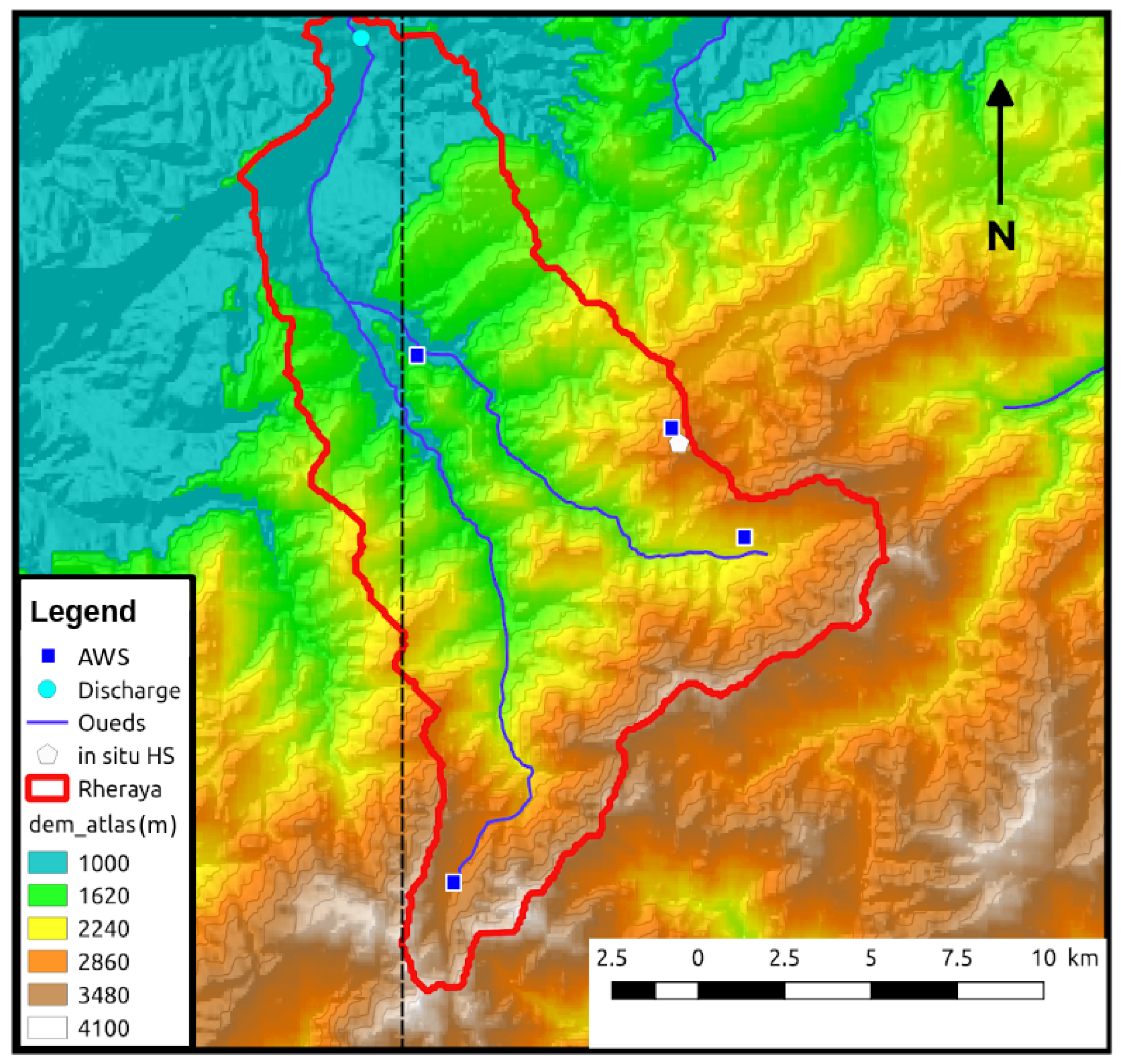
2.1. Study Area

The study area is the Rheraya catchment in the High Atlas Mountains of Morocco (Figure 1). The catchment elevation ranges from 1000 (river gauge station of Tahanaout) to 4167 m (Mount Toubkal, the highest peak in the North Africa). The Rheraya river discharge at Tahanaout is strongly influenced by the snow melt contribution in spring (Figure 2). The discharge during the melt season between March and May represents about 50% of the annual discharge. The catchment is sparsely vegetated, except in the valley’s bottoms, where snowfalls rarely occur.
We selected the Rheraya catchment because it is the only catchment in the High Atlas with high elevation automatic weather stations [33]. The Rheraya catchment was also the study site of previous snow hydrology studies in Morocco [3,34,35].

2.2. Data

2.2.1. Topography and Land Cover

The 90 m Shuttle Radar Topography Mission (SRTM) digital elevation model was used after resampling it to 200 m spatial resolution by using cubic interpolation. The choice of the spatial resolution is based on a previous study in the Rheraya catchment [36], where we analyzed the trade-off between spatial resolution and the computation time. This study suggested that a distributed snow model with a grid coarser than 250 m is not able to capture the high spatial variability in the snow cover patterns due to the importance of the incoming solar radiation in the snowpack energy budget.
The land cover use data set is derived from European Space Agency Climate Change I (ESA-CCI). The majority of the area is bare soil.

2.2.2. Snow Cover Area

We queried all available Sentinel-2 snow covered area (SCA) products between January and July 2016 in the L2B-Snow collection of the Theia Land data center [37]. All snow products were derived from Sentinel-2A acquisitions since Sentinel-2B was only launched in 2017. The Rheraya catchment intersects tiles 29RNQ and 29RPQ, but we used only the products from tile 29RPQ since the tile 29RNQ only covers the low elevation area of the catchment where the snow is rarely observed. The downloaded snow products were clipped over the Rheraya catchment in their native projection (WGS-84 UTM 29N). To reduce the input/output operation time in the assimilation phase, we removed the products with a cloud cover higher than 70%. We obtained 13 SCA maps of the Rheraya catchment with a snow cover fraction ranging from 82% to 0% and a cloud fraction ranging from 0% to 66% (Table 1).
These SCA products were generated from Sentinel-2 images based on the MAJA/LIS processor [37]. The MAJA processor computes the surface reflectance and the cloud and cloud shadow mask [38]. The output of MAJA is a level-2A product, that is read by the LIS processor to determine the snow cover area at 20 m resolution [37]. The snow detection is performed using the “flat surface reflectances”, i.e., surface reflectances that were corrected to remove the first order effect of the topography. The snow classification in LIS uses the Normalized Difference Snow Index [39]:
NDSI = ρ green ρ SWIR ρ green + ρ SWIR ,
where ρ green (resp. ρ SWIR ) is the flat surface reflectance in the green channel (resp. SWIR at 1.6 μ m). The NDSI encapsulates the fact that almost only snow surfaces are very bright in the visible but dark in the shortwave infrared. The output of LIS is a single band raster resolution having four possible values: snow, no-snow, cloud and no-data. For further details, the reader can refer to [37].
We used the daily MODIS snow products (MOD10A1 collection 6) to validate the different simulations. These products have a spatial resolution close to 500 m and a daily revisit time. The MODIS products were post-processed to generate a gap-free time series of snow cover fraction images (SCF) [4,8]. First, the NDSI in each snow pixel was converted to SCF using the equation that was used in the collection 5 [40]
SCF = 0.01 + 1.45 × NDSI
Then, the data gaps due to cloud obstruction were interpolated with the algorithm of [8], which was specifically developed and validated in the High Atlas mountains. The products were finally clipped over the Rheraya catchment.

2.2.3. MERRA-2 Data

The meteorological forcing were taken from NASA’s second Modern-Era Retrospective analysis for Research and Applications (MERRA-2). MERRA-2 reanalysis data are widely used, including studies dealing with the assimilation of snow cover data [24,25,41]. MERRA-2 data have a spatial resolution of 0.5 × 0.625 and a temporal resolution of 1 hour. MERRA-2 includes the assimilation of satellite observations that were not available to MERRA and an improved representation of key variables for simulating snowpack evolution [10]. We extracted the precipitation, 2-m air temperature, 2-m specific humidity and 2-m wind speed in the four nearest grid cell of the Rheraya catchment. The post-processing steps to make MERRA-2 compatible with SnowModel are described in [4].

2.2.4. In Situ Observations

The hourly data from three automatic weather stations (AWS) were used as input to SnowModel to generate synthetic observations and as validation data (snow height at Oukaimeden). Table 2 summarizes the AWS characteristics and available data. We also used a continuous record of the snow height at Oukaimeden (3230 m.a.s.l.) measured by an acoustic snow gauge.
We also used the observed river discharge at the gauging station of Tahanaout (31.29 N, −7.96 E, 1048 m) provided by the Tensift river basin water agency (ABHT). A river stage device measures the height of the water three times per day. The gauging is performed once per month at best for logistical reasons. These measurements are known to have large errors given the difficulty to establish a robust stage-discharge relation in the Rheraya river, which has an unstable river bed.

3. Methods

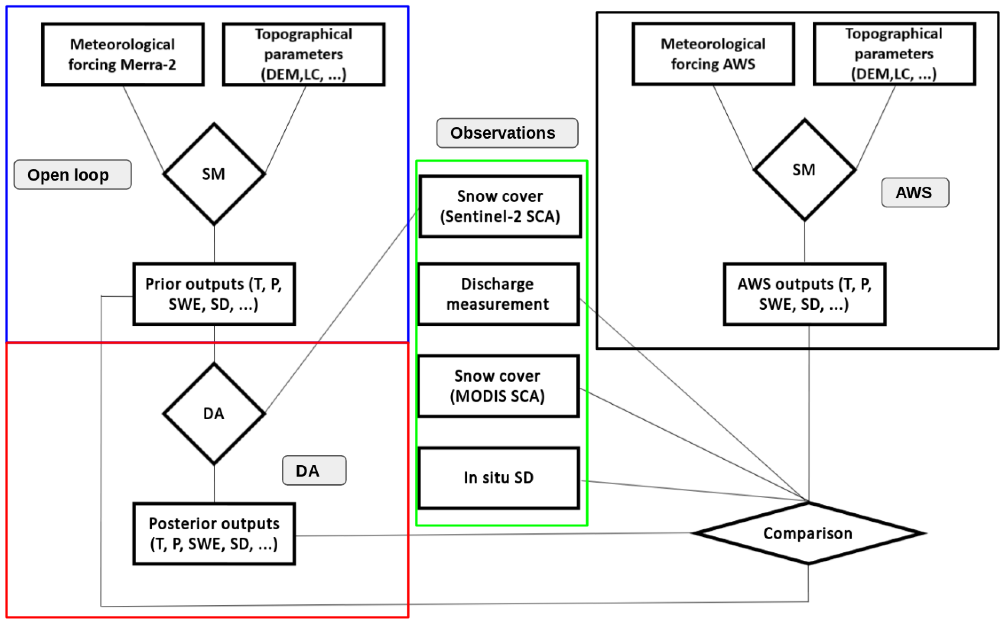
3.1. Validation Strategy

We focused on the 2015–2016 snow season. We defined three simulations:
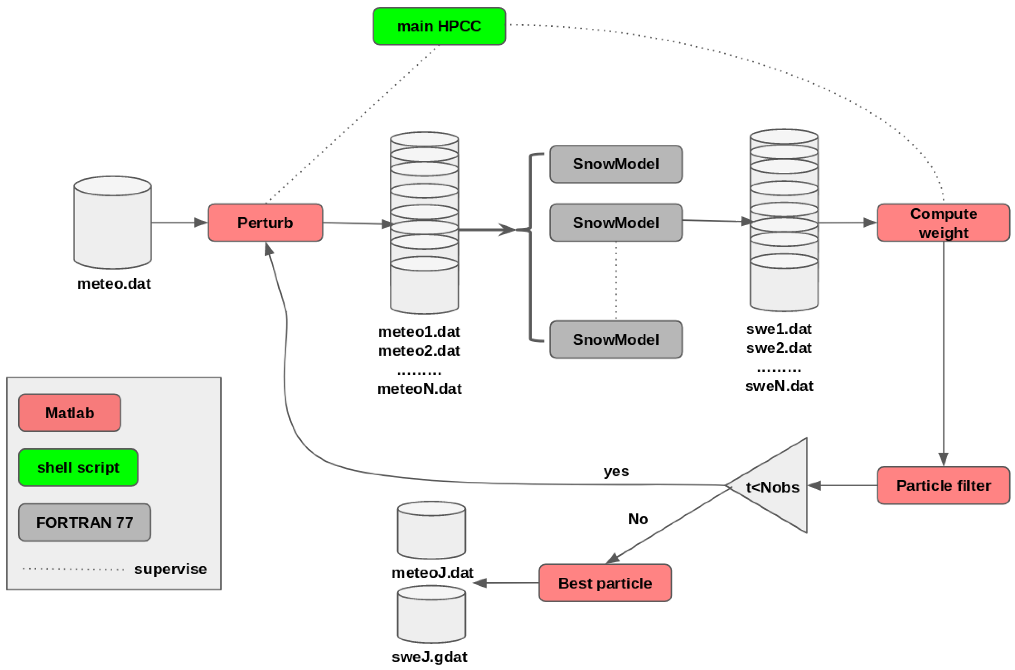
  • the open loop simulation (OL) was obtained by running SnowModel with downscaled MERRA-2 data as input. The output of this simulation is called the prior.
  • the data assimilation simulation (DA) was obtained in the same configuration as the open loop simulation but downscaled MERRA-2 forcings were perturbed to assimilate the Sentinel-2 snow cover maps through a particle filter. The output of this simulation is called the posterior.
  • the synthetic data simulation (referred to as AWS) was obtained by running SnowModel with in situ meteorological observations from the AWS. The output of this simulation was considered as an independent dataset to evaluate the effect of the assimilation.
The main input and output of the simulations is presented in Figure 3.
The performance of the DA was qualified by computing the RMSE (Equation (3)) and the Pearson correlation coefficient between the output of the DA scheme and the synthetic observations of air temperature, precipitation, SWE and SCA.
RMSE = 1 N i = 1 N ( X i X i truth ) 2
R = E [ X Y ] E [ X ] E [ Y ] E [ X 2 ] E [ X ] 2 E [ Y 2 ] E [ Y ] 2
where X i is the ith element of the vector X, and X i truth is the ith element of the synthetic observation vector X truth . E is the expectation. Y is the observation vector.
The output of the OL, DA and AWS were also compared to in situ observations of the snow height at Oukaimeden, the snow cover fraction of the catchment area from MODIS data and the river discharge at Tahanaout. Regarding the river discharge comparison, the challenge is that SnowModel does not simulate the water transfer from the snow melt to the streamflow. The runoff is the sum of the rain and melt water released from the snowpack. Given the complexity of the intermediate hydrological processes in the Rheraya catchment [3,42], we compared the observed discharge with the simulated runoff using 3-day averages. The Rheraya catchment has a low storage capacity because it is a mountainous catchment with steep slopes, thin soils and impermeable bedrock [35], therefore we considered that a 3-day average is sufficient. The simulated discharge was obtained by multiplying the simulated runoff by the catchment area.

3.2. Snowpack Model

We used SnowModel [43], a distributed energy-balance model, to simulate the snowpack evolution. The model was run at the hourly time step since the daily time step do not allow an accurate representation of the energy fluxes and determination of the precipitation phase [44]. SnowModel is composed of four sub-models: MicroMet, EnBal, SnowPack and SnowTran-3D. MicroMet distributes the meteorological forcing from station data on model grid using topography data [43]. EnBal solves the energy balance equation to compute the SWE evolution [29]. SnowPack computes the evolution of the snow depth and snowpack density [29]. SnowTran-3D computes the redistribution of the snow cover due to the wind [45].
In this work, SnowTran-3D was not activated because of its high computational cost. However, the assimilation scheme is compatible with SnowTran-3D. In addition, the assimilation scheme is not dependent upon the snowpack model itself, i.e., submodels EnBal and SnowPack could be replaced by another implementation of a snowpack model. Although our assimilation scheme does not depend on the type of snowpack model, it is closely linked to MicroMet (as explained in Section 3.4). This is why we focus below on the description of MicroMet submodel only.
In MicroMet, a DEM is used to correct the effect of elevation on air temperature, humidity and precipitation. In the case of the air temperature, the following equation is used:
T x = T s t n τ ( Z x Z s t n )
where T s t n is the air temperature at the station, Z s t n the station elevation, T x ( C) the air temperature in the target grid cell, Z x the elevation of the grid cell. τ is the temperature lapse rate ( C · km 1 ), which depends on the month of the year. As a first step, MicroMet adjusts the station data to a common elevation Z = 0 using Equation (5). Then, the temperature is interpolated using a Gaussian distance-dependent weighting function to the model grid [46]. Finally, Equation (5) is used again to adjust the gridded temperatures values back to the actual elevation taken from the DEM.
The same method is used for the relative humidity and precipitation. The relative humidity at the station is first converted to dew point temperature. The same function as for the air temperature is used to account for elevation (Equation (5), but with different lapse rate values. In the case of the precipitation, a different function of elevation is used:
P x = P s t n × [ 1 + χ ( Z x Z s t n ) ] [ 1 χ ( Z x Z s t n ) ]
where P s t n is the precipitation at the station, P x (mm) the precipitation in the target grid cell, Z x the elevation of the grid cell. χ is the precipitation correction factor (km 1 ), which also depends on the month of the year. The shortwave and longwave radiations are derived from the interpolated temperature and humidity on each grid cell accounting for the effect of the slope and orientation of the terrain [43]. The performance of MicroMet in a high-mountain semi-arid area was evaluated by Gascoin et al. [47]. The results of this study indicate that the uncertainties in the meteorological inputs due to MicroMet spatial interpolation are typically lower than the expected uncertainties in MERRA-2 data.
As noted above, MicroMet was originally designed to spatially distribute meteorological variables from weather station measurements. However it can also be used to downscale large scale meteorological data like MERRA-2 data. In this case, the MERRA-2 data are simply considered as the meteorological measurements of a virtual weather station that is located in the center of the MERRA-2 grid cell. The elevation of the virtual station is calculated from the surface geopotential height of the MERRA-2 cell. This approach was successfully applied in the High-Atlas [4] and in the Andes [12].
Preliminary sensitivity tests revealed that the parameterization of the precipitation solid fraction caused significant biases in the simulated snow cover area after the snowfalls. Excessive model biases should be corrected as much as possible to make the assimilation scheme efficient. By default, MicroMet uses a temperature threshold of 2 C to distinguish between solid and liquid precipitation [43]. We found that theses biases could be reduced by enhancing the default parameterization in SnowModel to account for the influence of the relative humidity on the precipitation phase using the empirical relation of Froidurot et al. [48]:
F s = 1 1 + e γ RH + β T + α
where F s is the solid fraction in the total precipitation, RH is the relative humidity in % and T the 2 m air temperature during the same time step. The parameters α , γ , β were optimized on a different snow season. We chose the 2008–2009 snow season for which we dispose of an accurate time series of high resolution SCA maps from Formosat-2 data [8]. A set of 200 ( α , γ , β ) triplets were generated in the intervals [22.00, 26.00], [−2.80, −2.40], [−0.25, −0.20] by Monte-Carlo sampling and used as parameters of the same SnowModel run as in [36]. These intervals were chosen following the recommendations of Froidurot et al. [48]. The optimization was done using the same model configuration as presented in [13]. We used the Heidle Skill Score (HSS) [49] between the simulated snow cover area and the Formosat-2 SCA maps over the entire study period to identify the optimal parameters triplet ( α = 25, β = −2.5, γ = −0.2).

3.3. SWE-SCA Conversion

We define the SCA as a binary variable indicating the presence (SCA = 1) or absence (SCA = 0) of snow in a grid cell, and the SCF as a continuous variable indicating the snow covered fraction of a grid cell. The SCA or the SCF are not standard outputs of SnowModel hence must be derived from the simulated SWE or snow depth. This transformation is done through a “snow depletion curve”. There are several snow depletion curve formulations in the literature [50,51], and their parameters are poorly known especially in the context of the High Atlas. In addition snow depletion curves were mostly developed for low to mid-resolution imagery like MODIS. Therefore, in this study we chose to assimilate the SCA rather than the SCF to reduce the importance of the snow depletion curve equation and parameters.
First, we compute the SCF at the grid cell level using the snow depletion curve of Zaitchik and Rodell [19], also used by Thirel et al. [21]:
SCF = min ( 1 [ exp ( τ SWE SWE SCF = 1 ) SWE SWE SCF = 1 exp ( τ ) ] , 1.0 )
where SWE is the snow water equivalent in the grid cell, τ is the snow distribution shape parameter relating the total amount of snow in the grid cell to the percent snow cover within the grid cell (by default it is set to 4.0 [21]). SWE SCF = 1 defines the minimum SWE to reach a full snow coverage within the grid cell, whose value depends on the land cover. In this study we used the value for bare soil (SWE SCF = 1 = 13 mm). The grid cell was considered as snow covered if the SCF is greater than a fixed value SCF 0 , i.e.,
SCA = u [ SCF SCF 0 ]
where u is the discrete form of the Heaviside function. SCF 0 was set to 0.25.

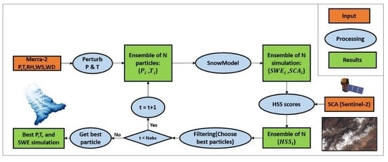
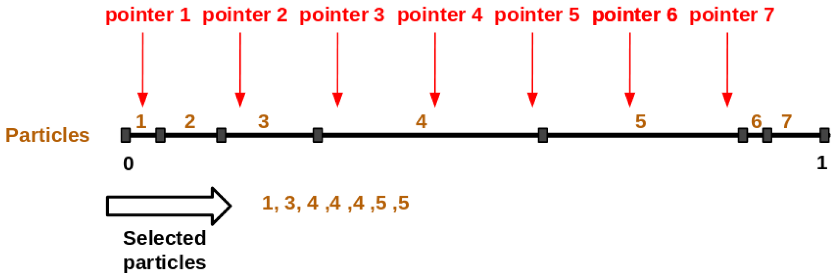
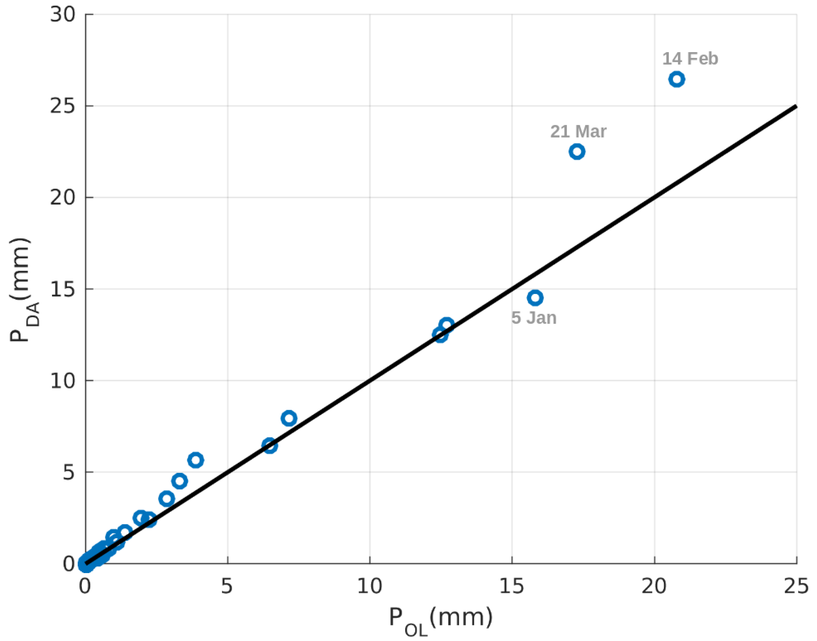
3.4. Data Assimilation Algorithm

In this study, the data assimilation scheme is used to reduce the biases in air temperature and precipitation. Let x the state vector containing a discrete approximation of the SWE, air temperature, precipitation. The basis of the particle filter is to seek the best estimation of the prognostic variables, by generating an ensemble of N e n s random draws (particles) x i where i [ 1 : N e n s ] . These particles are propagated through SnowModel whenever an observation (here a Sentinel-2 snow product) is available. At each observation date, a specific normalized weight is assigned to every particle [32,52]:
w i , j = 1 2 σ 2 π e ( ϵ i , j ) 2 2 σ 2
where w i , j is the weight of the ith particle at the jth observation date, σ is the standard deviation of the observation error. We assume that σ is constant throughout the study period. Here σ was set to 0.15 based on the comparison with very high resolution images in the Alps and a visual inspection of the snow products in our study area [37].
ϵ i , j is often defined as the difference between the spatial average of the observed and modeled SCF [31]. Here, we aim to take into account the differences between the model and the observations at the grid cell level (i.e., on a pixel basis) when defining the quality of each particle. Hence we chose to derive ϵ i , j from the Heidle skill score (HSS), a statistical index based on the confusion matrix, which is often used to evaluate the skills of snow remote sensing products at the pixel level [49]:
HSS = 2 ( T P × T N F P × F N ) ( T P + F P ) × ( F P + T N ) + ( T P + F N ) ( F N + T N )
where T P , T N , F P , F N are the number of true positive, true negative, false positive and false negative pixels, respectively. The perfect simulation has an HSS equal to 1 while the worst has an HSS close to 0. Hence, ϵ i , j is defined as:
ϵ i , j = 1 HSS i , j .
Subsequently, each weight is updated using
w i , j * = j = 1 n obs w i , j
where w i , j * is the updated value of the weight, n obs is the number of assimilated observations until this time step (including the jth). Thereafter the weights are normalized using:
W i = w i , j * i = 1 N w i
where W i is the updated normalized weight.
After computing the weights, the particle filter removes particles with low weight and duplicates particles with high weight to estimate the posterior distribution of the state vector. This step is called resampling. Many resampling algorithms exist (see a review by Douc and Cappé [53]). The most used algorithm in hydrological studies is the stochastic universal sampling (SUS) method, due to the ease of its implementation, its low computational time and also its satisfying results [54,55].
First, a vector containing the cumulative sum of W i is computed. Then, N pointers spaced by 1 / N are used to select the particles in this space (Figure 4). This enables to preferentially select a particle with a high weight given that this particle will span a larger segment of this space, hence particles with the highest weight will be duplicated. The selected particles are thereafter perturbed as explained in Section 3.4.1.
An issue arises if all particles have equivalent weights, e.g., if the domain is fully snow covered or snow-free. In this case, every particle is equally likely to be selected for the next assimilation window, which will prevent the creation of new particles since the number of particles must remain constant. Therefore, we modified the SUS to select, at each assimilation date, only 50% of the particles for the next assimilation window, i.e., we use only N S U S = N e n s / 2 pointers instead of N e n s . Thus, each selected particle is duplicated at least once.
Figure 5 shows the difference between the standard SUS resampling and the enhanced resampling in such a case of equivalent particle weights. In the standard algorithm, only one particle can be perturbed in the next step, whereas in the enhanced algorithm, three particles can be perturbed. This will increase the probability to obtain a better estimation of the state vector for the next assimilation step.
To summarize, we present the different steps of the computational implementation of the DA scheme as follows, and also illustrate them in Figure 6.
  • Sample N e n s particles x i by perturbing MERRA-2 precipitation and temperature.
  • Integrate all particles in SnowModel forward time (from t to t + 1 ).
  • Calculate the weights according to Equation (14).
  • Resample the particles with the enhanced SUS method.
  • Get the new N e n s particles x i . Repeat steps 1,2,3,4 sequentially until the end of observations.
  • Choose the particle with the maximum weight. The model output (SWE) that correspond to the most likely S W E t r u e state.

3.4.1. Ensemble of Meteorological Forcings

At each assimilation step, the MERRA-2 air temperature and precipitation are perturbed to generate an ensemble of meteorological forcing spanning the next assimilation window. It is important to emphasize that the perturbation is done before the downscaling by MicroMet, i.e., from the coarse scale MERRA-2 data, which are considered as virtual station measurements (Section 3.2).
For the air temperature, the perturbation is done by adding a white noise with zero mean and standard deviation of 2 C [18,31]. The precipitation data were perturbed by a multiplicative correction factor randomly sampled between 0.75 and 1.5 [56].

3.5. Implementation

The DA workflow uses code in Matlab, Fortran and shell scripts. The scheme was implemented in the CNES high performing computing cluster (HPCC). The main script uses the Portable Batch System (PBS Pro) job scheduler to execute the different steps. As a first step, the main HPCC PBS script creates N e n s perturbed meteorological forcing files (ASCII) from the initial meteorological file. Thereafter, N e n s simulations are performed with SnowModel in parallel (Figure 7). This allows to get N e n s of SWE simulations (GDAT binary files). For each particle the SWE is converted to SCA, then its weight is computed based on the observed snow cover area (GeoTiff). Finally, all particles enter the particle filtering process. These steps are repeated until the end of the observations (Figure 7). The PBS script was configured to request 8000 Mbytes of memory and 1 CPU per node. The whole DA process takes approximately 2 h.

4. Results

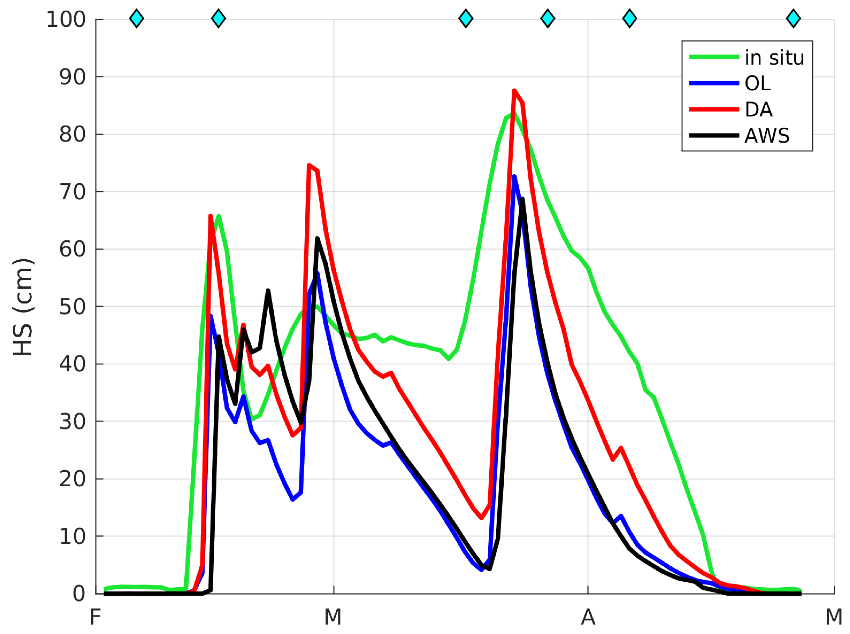
4.1. Comparison to In Situ Snow Height

The different simulations captured the overall snow height evolution at Oukaimeden (Figure 8), however the DA simulation outperformed the OL and AWS simulation in terms of correlation and RMSE (Table 3).
There remain large discrepancies from the end of February to the mid-March even in the DA simulation. Over the same period there is no assimilation data. In the three cases the melting rates were too high especially in March. By contrast, the DA simulation captured well the snow height peaks on 16 February and 26 March. Both peaks occurred between two successive Sentinel-2A acquisitions (7 and 17 February, 18 and 28 March, Table 1).

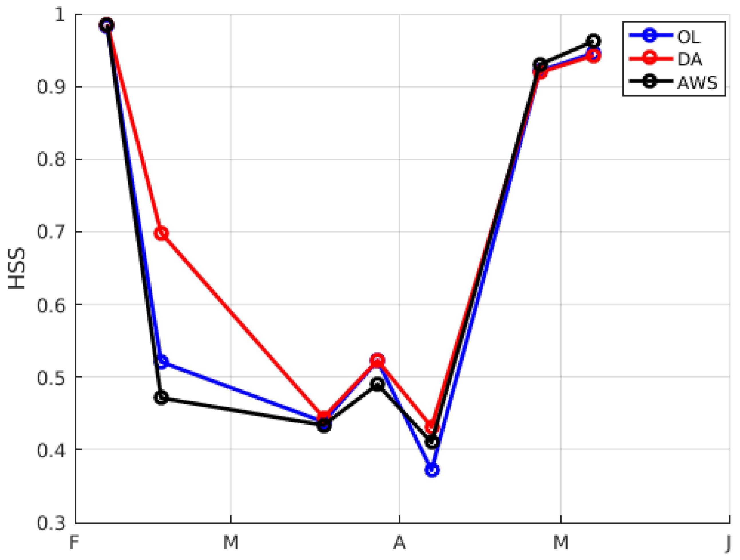
4.2. Comparison to MODIS

Figure 9 shows the evolution of the snow covered fraction of the Rheraya catchment over the study period from the three simulations and from MODIS observations. The simulated snow covered fraction of the catchment was obtained by taking the average of the SCF in every grid cell, which was obtained by applying Equation (8). The three simulations reproduce well the MODIS observations (Table 3). The DA cSCF is larger than the OL cSCF, meaning that the correction of the precipitation led to increase the snowfall. The RMSE and correlation both indicate that the DA has improved the realism of the simulation with respect to the OL simulation (Table 3). The DA simulation is close to the AWS forcing but it is also slightly better in terms of RMSE and correlation.

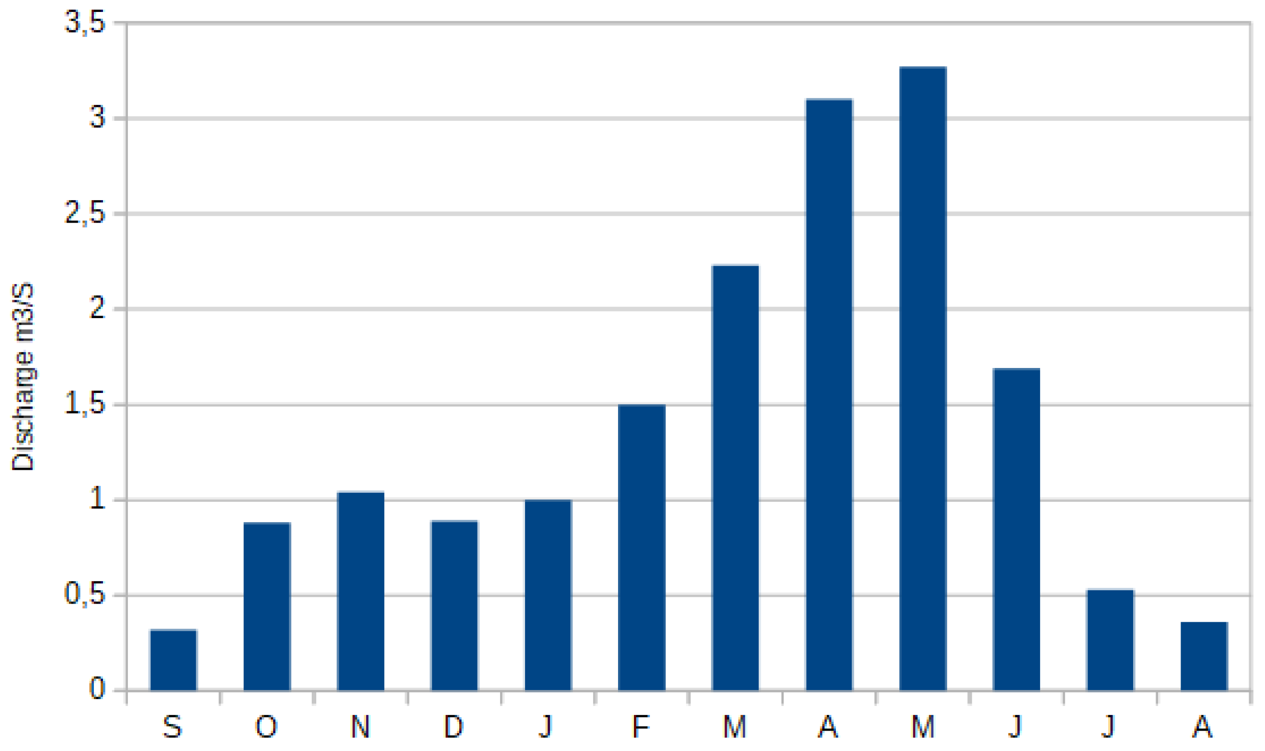
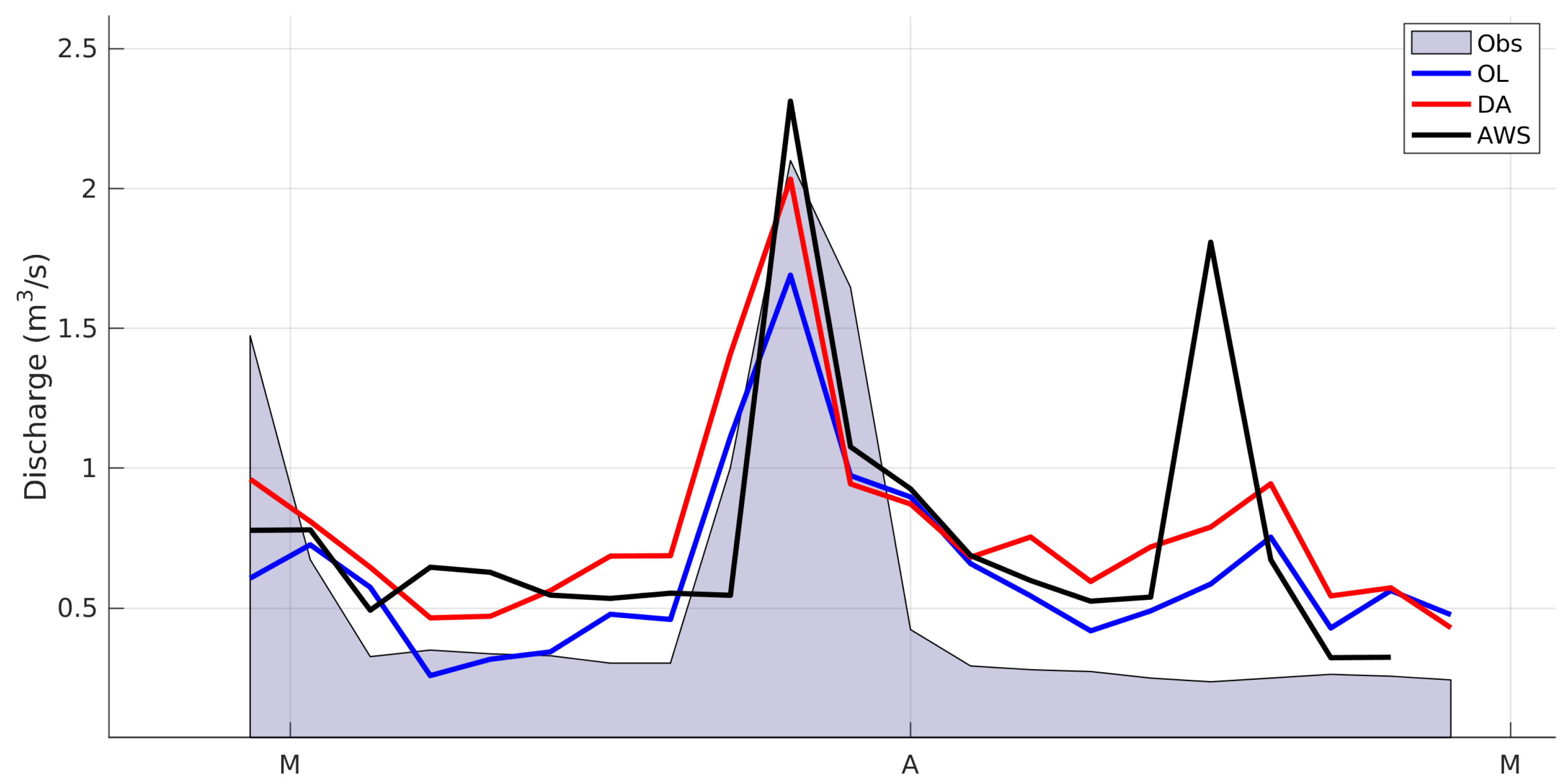
4.3. Comparison to Discharge Observations

Despite the crude approach to compute the discharge from the model output, the three simulations provide a realistic representation of the discharge at the 3-day time step. The DA simulation better captures the spring melt flood at the end of March (Figure 10). In addition, the AWS simulation has a large error in mid-April (an excessive melt), which is not present in the OL and DA simulations.

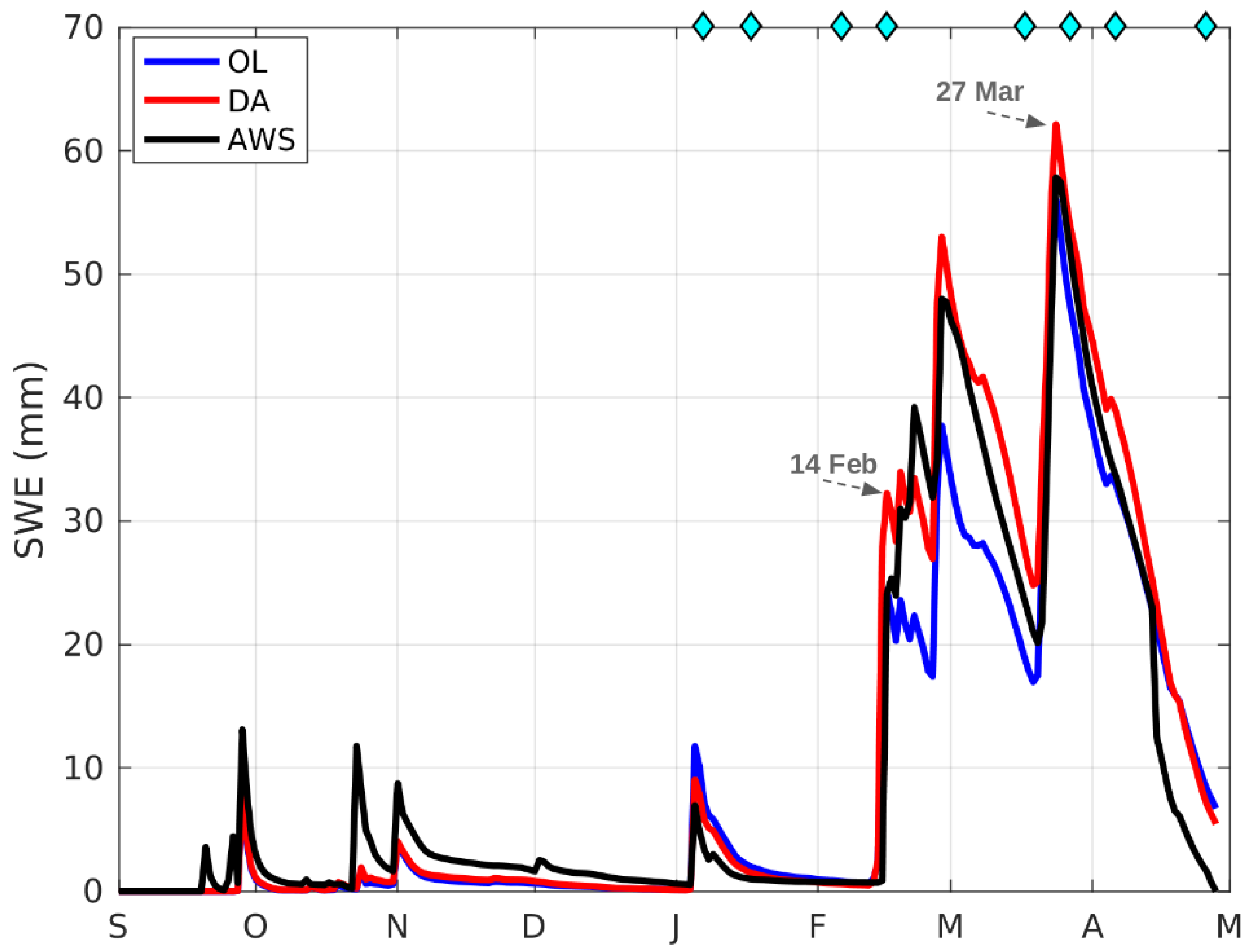
4.4. Comparison to the AWS Simulation

As explained in Section 3.1, we use the AWS simulation to assess the effect of the data assimilation on the SWE, air temperature and precipitation.
Figure 11 shows the evolution of the mean SWE over the Rheraya catchment from the three simulations. The difference between the DA SWE and OL SWE is highest between mid-February to mid-March. The DA has led to a significant increase in the simulated SWE with respect to the OL simulation. As a result, the DA SWE is closer to the AWS SWE during the same period. As shown in Figure 12, the higher SWE in the DA run is the result of higher precipitations, in particular the DA has increased the precipitation rate of the two major events on 14 February and 27 March. However, despite these differences in the accumulation period, the DA and OL simulations produced a similar SWE in the end of the melt season. This can be explained by the differences in evolution of the air temperature over the melt season (Figure 13). The mean air temperature in the DA simulation is higher than the one of the OL simulation between February to May, which increased the melting rate in the DA simulation.
On 5 January, we note that the DA has reduced the OL precipitation (Figure 12), which is consistent with the AWS simulation (Figure 11).

5. Discussion

The results show that the data assimilation scheme has reduced the bias and increased the correlation with two independent observation datasets of snow height and snow cover area. However, these observations provide only a partial evaluation of the simulations: (i) the snow height was measured only at the Oukaimeden weather station, therefore it is not necessarily representative of the snow height evolution over the entire catchment, even at similar elevations; (ii) a better agreement with the MODIS snow cover area does not necessarily mean that other snowpack properties like the SWE were better simulated. However, the combination of these observations suggest that the assimilation improves the model outputs.
The comparison with the synthetic data (AWS simulation) showed that MERRA-2 provided a good estimate of the meteorological forcing in agreement with a previous study in the neighbouring catchment of the Ourika catchment [4]. This means that there was a relatively low bias in the prior precipitation and air temperature, which could have caused otherwise a divergence in the posterior SWE. Yet, the assimilation generally tended to increase the precipitation and SWE (Figure 12 and Figure 14). However, it decreased the SWE in the highest area of the catchment near the Toubkal peak (Figure 14). This is consistent with the fact that MicroMet uses a crude representation of the orographic enhancement of the precipitation (Section 3.2). If the weather stations used in the interpolation are located at lower elevations, MicroMet lapse rate formulation can lead to overestimated distribution of the precipitation at high elevation without assimilation (Equation (6)). Here the elevation of MERRA-2 virtual stations ranges between 836 m and 1892 m, whereas the elevations in southern part of the catchment exceed 3000 m.a.s.l. During the melt season, the data assimilation also increased the air temperature (Figure 13) and as a result the air temperature is more consistent with the AWS simulation. Consequently, it means that the posterior air temperature is more consistent with in situ observations of the air temperature.
Figure 15 shows the evolution of the HSS with respect to the Sentinel-2 data over the simulation period. As expected, the HSS of the DA simulation is higher than the OL HSS since the HSS was used in the function to weight the particles during the assimilation. The median of the HSS values is 0.72 for OL, 0.81 for DA and 0.71 for AWS. The improvement is mostly significant on 17 February and 07 April. The assimilation of the 17 February Sentinel-2 image in particular has caused an increase in the SWE which persisted until mid-March (Figure 11). This image was captured only 3 days after the precipitation event of the 14 February, the largest precipitation event of the study period (Figure 12). As a result this observation was important in the general performance of the assimilation scheme.
The approach presented in this study is based on the downscaling of large scale MERRA-2 data with MicroMet. Each MERRA-2 grid cell is considered as a virtual station. In the proposed data assimilation scheme, the meteorological forcing is perturbed at each virtual station before downscaling to the resolution of the snowpack model. This enables to restrain the number of particles (and thus the computation cost), in comparison with a data assimilation scheme which perturbs the forcing at the model grid cell level. Another advantage of this approach is that it guarantees a spatially smooth distribution of the posterior SWE, because MicroMet distributes the meteorological forcing using an optimal Gaussian distance-dependent weighting function [43,46]. However, localized weather phenomenon like convective precipitation events might not be corrected correctly with this approach. Another important limitation is related to the generation of the perturbed precipitation data. Here we used a stochastic multiplicative factor, which means that if the MERRA-2 precipitation is zero, the perturbed precipitation data is unchanged. Hence, the success of the particle filter is strongly dependent upon the quality of the prior precipitation from MERRA-2. In this study, we found that MERRA-2 provided a good first guess for the snow season 2015-2016. A previous study in the High Atlas showed that the general quality of MERRA-2 data is higher over the most recent years, probably due to the increasing amount of analyzed weather satellite data [4].
The assimilation scheme has also a number of known deficiencies in its non-stochastic parts. In particular, the MicroMet submodel does not simulate a number of meteorological processes, which can influence the snowpack energy balance like gravity-driven winds, thermal inversions, or differences between leeward and windward slopes in precipitations, which may create a bias even at a catchment level. In addition, the calculation of the radiation budget does not account for projected shadows and reflected light from the surrounding slopes. The energy balance model does not account for radiative forcing due to light absorbing impurities. However, the main source of uncertainty is probably due to the lack of knowledge in the variability of the surface roughness length across the domain.

6. Conclusions

We presented a new data assimilation scheme to integrate Sentinel-2 snow cover area in the simulation of the SWE in the High Atlas. The scheme is a particle filter with a modified stochastic universal sampling. The snowpack model is the distributed snow evolution model SnowModel. The method is based only on remote sensing and global climate data hence it does not require ground measurements. The results showed that the assimilation has improved the simulation of the snow cover, although this study covered only the 2015–2016 snow season before the launch of Sentinel-2B when the 5-day revisit time of the Sentinel-2 mission was not yet achieved. Since late 2017, both Sentinel-2 satellites are acquiring data over all land masses at full systematic 5-day revisit. This should increase the value of Sentinel-2 observations for snow studies in particular in areas of transient snow cover like semi-arid and Mediterranean climate mountain areas. Indeed, our study showed that a single image could have a significant positive impact on the posterior SWE, e.g., if it is acquired shortly after a snowfall event.
Here we focused on the assimilation of the snow cover area because it is easily retrieved from widely available optical remote sensing observations. However, assimilating the snow cover area only can lead to ambiguous posterior estimations [57]. For instance, if the prior underestimates the snow cover duration at high elevation with respect to satellite observations, this can be corrected by decreasing the air temperature (to reduce melting rate) but also by increasing the precipitation (to increase snow accumulation). This equifinality issue can be tackled by incorporating additional observations. In particular, we argue that even sporadic SWE or snow height measurements (e.g., snow courses) would drastically reduce the uncertainties in the posterior SWE. If such measurements are not performed by operational weather and water agencies, an option is to use crowd-sourced snow data. Our data assimilation scheme can be adapted to integrate this kind of observations because it is based on a distributed snow modelling. Additional remote sensing products like wet snow areas from Sentinel-1 could also be incorporated. Finally, additional meteorological variables could be updated using the same assimilation scheme, e.g., the shortwave radiation, which is an important driver of the snowpack energy-balance in the High Atlas. In this perspective, further model developments are also required to enhance the representation of the radiation processes in SnowModel, including the effect of Saharan dust deposition on snow albedo.
The continuous improvement of global-scale reanalyzes and the increasing availability of remote sensing data should lead to a better characterization of the SWE in more catchments in High Atlas even without ground measurements. Ultimately, this should contribute to a better knowledge of the water resources for the local communities.

Author Contributions

M.W.B. and S.G. designed the study. M.W.B. developed the data assimilation scheme. M.W.B. and S.G. analyzed the results. M.W.B. and S.G. wrote the paper with inputs from L.H.

Funding

This research was funded by Centre National d’Etudes Spatiales (CNES) and the Région Occitanie.

Acknowledgments

M.W.B. acknowledges the CNES and the Région Occitanie for funding his Ph.D. grant. S.G. acknowledges support by the CNES through the Tosca programme. We thank the Agence du Bassin Hydraulique du Tensift and Laboratoire Mixte International (LMI TREMA) for providing the discharge and meteorological data. The MERRA-2 data used in this study have been provided by the Global Modeling and Assimilation Office (GMAO) at NASA Goddard Space Flight Center. Sentinel-2 is a mission of the European Commission Copernicus program operated by the ESA. We thank the Theia Land data center for providing the Sentinel-2 snow products.

Conflicts of Interest

The authors declare no conflict of interest.

References

  1. Viviroli, D.; Dürr, H.H.; Messerli, B.; Meybeck, M.; Weingartner, R. Mountains of the world, water towers for humanity: Typology, mapping, and global significance. Water Resour. Res. 2007, 43. [Google Scholar] [CrossRef] [Green Version]
  2. Schulz, O.; De Jong, C. Snowmelt and sublimation: Field experiments and modelling in the High Atlas Mountains of Morocco. Hydrol. Earth Syst. Sci. 2004, 8, 1076–1089. [Google Scholar] [CrossRef]
  3. Boudhar, A.; Hanich, L.; Boulet, G.; Duchemin, B.; Berjamy, B.; Chehbouni, A. Evaluation of the snowmelt runoff model in the Moroccan High Atlas Mountains using two snow-cover estimates. Hydrol. Sci. J. 2009, 54, 1094–1113. [Google Scholar] [CrossRef]
  4. Baba, M.; Gascoin, S.; Jarlan, L.; Simonneaux, V.; Hanich, L. Variations of the Snow Water Equivalent in the Ourika Catchment (Morocco) over 2000–2018 Using Downscaled MERRA-2 Data. Water 2018, 10, 1120. [Google Scholar] [CrossRef]
  5. Fayad, A.; Gascoin, S.; Faour, G.; Fanise, P.; Drapeau, L.; Somma, J.; Fadel, A.; Al Bitar, A.; Escadafal, R. Snow observations in Mount Lebanon (2011–2016). Earth Syst. Sci. Data 2017, 9, 573. [Google Scholar] [CrossRef]
  6. Marks, D.; Domingo, J.; Susong, D.; Link, T.; Garen, D. A spatially distributed energy balance snowmelt model for application in mountain basins. Hydrol. Process. 1999, 13, 1935–1959. [Google Scholar] [CrossRef]
  7. Fassnacht, S.R.; López-Moreno, J.I.; Ma, C.; Weber, A.N.; Pfohl, A.K.D.; Kampf, S.K.; Kappas, M. Spatio-temporal snowmelt variability across the headwaters of the Southern Rocky Mountains. Front. Earth Sci. 2017, 11, 505–514. [Google Scholar] [CrossRef]
  8. Marchane, A.; Jarlan, L.; Hanich, L.; Boudhar, A.; Gascoin, S.; Tavernier, A.; Filali, N.; Le Page, M.; Hagolle, O.; Berjamy, B. Assessment of daily MODIS snow cover products to monitor snow cover dynamics over the Moroccan Atlas mountain range. Remote Sens. Environ. 2015, 160, 72–86. [Google Scholar] [CrossRef]
  9. Dozier, J.; Bair, E.H.; Davis, R.E. Estimating the spatial distribution of snow water equivalent in the world’s mountains. Wiley Interdiscip. Rev. Water 2016, 3, 461–474. [Google Scholar] [CrossRef]
  10. Gelaro, R.; McCarty, W.; Suárez, M.J.; Todling, R.; Molod, A.; Takacs, L.; Randles, C.A.; Darmenov, A.; Bosilovich, M.G.; Reichle, R.; et al. The Modern-Era Retrospective Analysis for Research and Applications, Version 2 (MERRA-2). J. Clim. 2017, 30, 5419–5454. [Google Scholar] [CrossRef]
  11. Durand, M.; Molotch, N.P.; Margulis, S.A. A Bayesian approach to snow water equivalent reconstruction. J. Geophys. Res. Atmos. 2008, 113. [Google Scholar] [CrossRef] [Green Version]
  12. Mernild, S.H.; Liston, G.E.; Hiemstra, C.A.; Malmros, J.K.; Yde, J.C.; McPhee, J. The Andes Cordillera. Part I: Snow distribution, properties, and trends (1979–2014). Int. J. Climatol. 2017, 37, 1680–1698. [Google Scholar] [CrossRef]
  13. Baba, W.; Gascoin, S.; Hanich, L.; Kinnard, C. Contribution of high resolution remote sensing data to the modeling of the snow cover the in Atlas Mountains. In EGU General Assembly Conference Abstracts; EGU General Assembly: Vienna, Austria, 2017; Volume 19, p. 19250. [Google Scholar]
  14. Reichle, R.H.; Liu, Q.; Koster, R.D.; Draper, C.S.; Mahanama, S.P.; Partyka, G.S. Land surface precipitation in MERRA-2. J. Clim. 2017, 30, 1643–1664. [Google Scholar] [CrossRef]
  15. Dietz, A.J.; Kuenzer, C.; Gessner, U.; Dech, S. Remote sensing of snow—A review of available methods. Int. J. Remote Sens. 2012, 33, 4094–4134. [Google Scholar] [CrossRef]
  16. Dumont, M.; Gascoin, S. Optical remote sensing of snow cover. In Land Surface Remote Sensing in Continental Hydrology; Elsevier: Amsterdam, The Netherlands, 2017; pp. 115–137. [Google Scholar]
  17. Andreadis, K.M.; Lettenmaier, D.P. Assimilating remotely sensed snow observations into a macroscale hydrology model. Adv. Water Resour. 2006, 29, 872–886. [Google Scholar] [CrossRef]
  18. Clark, M.P.; Rupp, D.E.; Woods, R.A.; Zheng, X.; Ibbitt, R.P.; Slater, A.G.; Schmidt, J.; Uddstrom, M.J. Hydrological data assimilation with the ensemble Kalman filter: Use of streamflow observations to update states in a distributed hydrological model. Adv. Water Resour. 2008, 31, 1309–1324. [Google Scholar] [CrossRef]
  19. Zaitchik, B.F.; Rodell, M. Forward-looking assimilation of MODIS-derived snow-covered area into a land surface model. J. Hydrometeorol. 2009, 10, 130–148. [Google Scholar] [CrossRef]
  20. De Lannoy, G.J.; Reichle, R.H.; Arsenault, K.R.; Houser, P.R.; Kumar, S.; Verhoest, N.E.; Pauwels, V.R. Multiscale assimilation of Advanced Microwave Scanning Radiometer—EOS snow water equivalent and Moderate Resolution Imaging Spectroradiometer snow cover fraction observations in northern Colorado. Adv. Water Resour. 2012, 48. [Google Scholar] [CrossRef]
  21. Thirel, G.; Salamon, P.; Burek, P.; Kalas, M. Assimilation of MODIS snow cover area data in a distributed hydrological model using the particle filter. Remote Sens. 2013, 5, 5825–5850. [Google Scholar] [CrossRef]
  22. Margulis, S.A.; Girotto, M.; Cortés, G.; Durand, M. A particle batch smoother approach to snow water equivalent estimation. J. Hydrometeorol. 2015, 16, 1752–1772. [Google Scholar] [CrossRef]
  23. Stigter, E.E.; Wanders, N.; Saloranta, T.M.; Shea, J.M.; Bierkens, M.F.; Immerzeel, W.W. Assimilation of snow cover and snow depth into a snow model to estimate snow water equivalent and snowmelt runoff in a Himalayan catchment. Cryosphere 2017, 11, 1647. [Google Scholar] [CrossRef]
  24. Toure, A.M.; Reichle, R.H.; Forman, B.A.; Getirana, A.; De Lannoy, G.J. Assimilation of MODIS Snow Cover Fraction Observations into the NASA Catchment Land Surface Model. Remote Sens. 2018, 10, 316. [Google Scholar] [CrossRef] [PubMed]
  25. Cortés, G.; Margulis, S. Impacts of El Niño and La Niña on interannual snow accumulation in the Andes: Results from a high-resolution 31 year reanalysis. Geophys. Res. Lett. 2017, 44, 6859–6867. [Google Scholar] [CrossRef]
  26. Gascoin, S.; Hagolle, O.; Huc, M.; Jarlan, L.; Dejoux, J.F.; Szczypta, C.; Marti, R.; Sánchez, R. A snow cover climatology for the Pyrenees from MODIS snow products. Hydrol. Earth Syst. Sci. 2015, 19, 2337–2351. [Google Scholar] [CrossRef] [Green Version]
  27. Gascon, F.; Bouzinac, C.; Thépaut, O.; Jung, M.; Francesconi, B.; Louis, J.; Lonjou, V.; Lafrance, B.; Massera, S.; Gaudel-Vacaresse, A.; et al. Copernicus Sentinel-2A calibration and products validation status. Remote Sens. 2017, 9, 584. [Google Scholar] [CrossRef]
  28. Drusch, M.; Del Bello, U.; Carlier, S.; Colin, O.; Fernandez, V.; Gascon, F.; Hoersch, B.; Isola, C.; Laberinti, P.; Martimort, P.; et al. Sentinel-2: ESA’s optical high-resolution mission for GMES operational services. Remote Sens. Environ. 2012, 120, 25–36. [Google Scholar] [CrossRef]
  29. Liston, G.E.; Elder, K. A distributed snow-evolution modeling system (SnowModel). J. Hydrometeorol. 2006, 7, 1259–1276. [Google Scholar] [CrossRef]
  30. Moradkhani, H.; Hsu, K.L.; Gupta, H.; Sorooshian, S. Uncertainty assessment of hydrologic model states and parameters: Sequential data assimilation using the particle filter. Adv. Water Resour. 2005, 41. [Google Scholar] [CrossRef] [Green Version]
  31. Leisenring, M.; Moradkhani, H. Snow water equivalent prediction using Bayesian data assimilation methods. Stoch. Environ. Res. Risk Assess. 2011, 25, 253–270. [Google Scholar] [CrossRef]
  32. van Leeuwen, P.J.; Künsch, H.R.; Nerger, L.; Potthast, R.; Reich, S. Particle filters for applications in geosciences. arXiv, 2018; arXiv:1807.10434. [Google Scholar]
  33. Jarlan, L.; Khabba, S.; Er-Raki, S.; Le Page, M.; Hanich, L.; Fakir, Y.; Merlin, O.; Mangiarotti, S.; Gascoin, S.; Ezzahar, J.; et al. Remote sensing of water resources in semi-arid mediterranean areas: The joint international laboratory TREMA. Int. J. Remote Sens. 2015, 36, 4879–4917. [Google Scholar] [CrossRef]
  34. Marchane, A.; Tramblay, Y.; Hanich, L.; Ruelland, D.; Jarlan, L. Climate change impacts on surface water resources in the Rheraya catchment (High Atlas, Morocco). Hydrol. Sci. J. 2017, 62, 979–995. [Google Scholar] [CrossRef]
  35. Hajhouji, Y.; Simonneaux, V.; Gascoin, S.; Fakir, Y.; Richard, R.; Chehbouni, A. Modélisation pluie-débit et analyse du régime d’un bassin versant semi-aride sous influence nivale. Cas du bassin versant du Rheraya (Haut Atlas, Maroc). La Houille Blanche 2018, 3, 49–62. [Google Scholar] [CrossRef]
  36. Baba, M.W.; Gascoin, S.; Kinnard, C.; Marchane, A.; Hanich, L. Effect of Digital Elevation Model Resolution on the Simulation of the Snow Cover Evolution in the High Atlas. 2018. Available online: https://osf.io/9zxqg/ (accessed on 4 December 2018).
  37. Gascoin, S.; Grizonnet, M.; Bouchet, M.; Salgues, G.; Hagolle, O. Theia Snow collection: high resolution operational snow cover maps from Sentinel-2 and Landsat-8 data. Earth Syst. Sci. Data Discuss. 2018, 2018, 1–31. [Google Scholar] [CrossRef]
  38. Lonjou, V.; Desjardins, C.; Hagolle, O.; Petrucci, B.; Tremas, T.; Dejus, M.; Makarau, A.; Auer, S. MACCS-ATCOR joint algorithm (MAJA). In Proceedings of the Remote Sensing of Clouds and the Atmosphere XXI, Edinburgh, UK, 26–29 September 2016; Volume 10001, p. 1000107. [Google Scholar]
  39. Dozier, J. Spectral signature of alpine snow cover from the Landsat Thematic Mapper. Remote Sens. Environ. 1989, 28, 9–22. [Google Scholar] [CrossRef]
  40. Hall, D.K.; Riggs, G.A.; Salomonson, V.V.; Barton, J.; Casey, K.; Chien, J.; DiGirolamo, N.; Klein, A.; Powell, H.; Tait, A. Algorithm Theoretical Basis Document (ATBD) for the MODIS Snow and Sea Ice-Mapping Algorithms. Nasa Gsfc 2001, 45. Available online: https://eospso.gsfc.nasa.gov/sites/default/files/atbd/atbd_mod10.pdf (accessed on 4 December 2018).
  41. Baldo, E. Towards Large-Scale Implementation of a High Resolution Snow Reanalysis over Midlatitude Montane Ranges. Ph.D. Thesis, University of California, Los Angeles, CA, USA, 2017. [Google Scholar]
  42. Chaponnière, A.; Boulet, G.; Chehbouni, A.; Aresmouk, M. Understanding hydrological processes with scarce data in a mountain environment. Hydrol. Process. 2008, 22, 1908–1921. [Google Scholar] [CrossRef] [Green Version]
  43. Liston, G.E.; Elder, K. A meteorological distribution system for high-resolution terrestrial modeling (MicroMet). J. Hydrometeorol. 2006, 7, 217–234. [Google Scholar] [CrossRef]
  44. Bair, E.H.; Rittger, K.; Davis, R.E.; Painter, T.H.; Dozier, J. Validating reconstruction of snow water equivalent in California’s Sierra Nevada using measurements from the NASA Airborne Snow Observatory. Adv. Water Resour. 2016, 52, 8437–8460. [Google Scholar] [CrossRef]
  45. Liston, G.E.; Haehnel, R.B.; Sturm, M.; Hiemstra, C.A.; Berezovskaya, S.; Tabler, R.D. Simulating complex snow distributions in windy environments using SnowTran-3D. J. Glaciol. 2007, 53, 241–256. [Google Scholar] [CrossRef]
  46. Barnes, S.L. A technique for maximizing details in numerical weather map analysis. J. Appl. Meteorol. 1964, 3, 396–409. [Google Scholar] [CrossRef]
  47. Gascoin, S.; Lhermitte, S.; Kinnard, C.; Bortels, K.; Liston, G.E. Wind effects on snow cover in Pascua-Lama, Dry Andes of Chile. Adv. Water Resour. 2013, 55, 25–39. [Google Scholar] [CrossRef] [Green Version]
  48. Froidurot, S.; Zin, I.; Hingray, B.; Gautheron, A. Sensitivity of precipitation phase over the Swiss Alps to different meteorological variables. J. Hydrometeorol. 2014, 15, 685–696. [Google Scholar] [CrossRef]
  49. Notarnicola, C.; Duguay, M.; Moelg, N.; Schellenberger, T.; Tetzlaff, A.; Monsorno, R.; Costa, A.; Steurer, C.; Zebisch, M. Snow cover maps from MODIS images at 250 m resolution, part 2: Validation. Remote Sens. 2013, 5, 1568–1587. [Google Scholar] [CrossRef]
  50. Liston, G.E. Representing subgrid snow cover heterogeneities in regional and global models. J. Clim. 2004, 17, 1381–1397. [Google Scholar] [CrossRef]
  51. Andreadis, K.M.; Clark, E.A.; Wood, A.W.; Hamlet, A.F.; Lettenmaier, D.P. Twentieth-century drought in the conterminous United States. J. Hydrometeorol. 2005, 6, 985–1001. [Google Scholar] [CrossRef]
  52. van Leeuwen, P.J. Nonlinear data assimilation in geosciences: An extremely efficient particle filter. Q. J. R. Meteorol. Soc. 2010, 136, 1991–1999. [Google Scholar] [CrossRef]
  53. Douc, R.; Cappé, O. Comparison of resampling schemes for particle filtering. In Proceedings of the 4th International Symposium on the Image and Signal Processing and Analysis, Zagreb, Croatia, 15–17 September 2005; pp. 64–69. [Google Scholar]
  54. Pencheva, T.; Atanassov, K.; Shannon, A. Modelling of a stochastic universal sampling selection operator in genetic algorithms using generalized nets. In Proceedings of the Tenth International Workshop on Generalized Nets, Sofia, Bulgaria, 5 December 2009; pp. 1–7. [Google Scholar]
  55. Noh, S.; Tachikawa, Y.; Shiiba, M.; Kim, S. Applying sequential Monte Carlo methods into a distributed hydrologic model: Lagged particle filtering approach with regularization. Hydrol. Earth Syst. Sci. 2011, 15, 3237–3251. [Google Scholar] [CrossRef]
  56. Charrois, L.; Cosme, E.; Dumont, M.; Lafaysse, M.; Morin, S.; Libois, Q.; Picard, G. On the assimilation of optical reflectances and snow depth observations into a detailed snowpack model. Cryosphere 2016, 10, 1021–1038. [Google Scholar] [CrossRef]
  57. Aalstad, K.; Westermann, S.; Schuler, T.V.; Boike, J.; Bertino, L. Ensemble-based assimilation of fractional snow-covered area satellite retrievals to estimate the snow distribution at Arctic sites. Cryosphere 2018, 17, 247–270. [Google Scholar] [CrossRef]
Figure 1. Elevations of the Rheraya catchment, and the location of discharge measurement (sky blue), in situ snow height (HS) and automatic weather stations (AWS). The dashed points refers to the intersection between Sentinel-2 images borders and the Rheraya.
Remotesensing 10 01982 g001
Figure 2. Mean monthly discharge (m 3 /s) of the Rheraya River at Tahanaout (river discharge data from the Agence du Bassin Hydraulique du Tensift (1974–2003).
Remotesensing 10 01982 g002
Figure 3. Simplified schematic illustrating the input and output of the DA scheme. SM refers to SnowModel. DA refers to data assimilation process and AWS refers to the simulation based on autmatic weather stations (AWS) data.
Remotesensing 10 01982 g003
Figure 4. Principle of the stochastic universal sampling method in the case of 7 particles [54]. The brown numbers identify each ith particle and the segment size is proportional to its normalized weight W i .
Remotesensing 10 01982 g004
Figure 5. Schema describing the weight calculation and resampling. (1): with initial SUS resampling. (2) with enhanced SUS method.
Remotesensing 10 01982 g005
Figure 6. Description of the data assimilation scheme used in this study.
Remotesensing 10 01982 g006
Figure 7. Description of the information technology (IT) implementation of the particle filter in this study.
Remotesensing 10 01982 g007
Figure 8. Comparison of the simulated and observed in situ snow height in Oukaimeden at the daily time step. The blue diamonds in the upper part of the figure indicate the date of the assimilated Sentinel-2 observations. OL: open loop snow height, DA: data assimilation snow height, AWS: modeled snow height using automatic weather stations forcing.
Remotesensing 10 01982 g008
Figure 9. Comparison of the simulated and observed snow covered fraction of the Rheraya catchment (cSCF) at the daily time step. The blue diamonds in the upper part of the figure indicate the date of the assimilated Sentinel-2 observations. OL: open loop sSCF, DA: data assimilation sSCF, AWS: modeled sSCF by using automatic weather stations data.
Remotesensing 10 01982 g009
Figure 10. Comparison of the simulated and observed discharge at Tahanaout (see Section 3.1). OL: open loop discharge, DA: data assimilation discharge, AWS: modeled discharge by using automatic weather stations data.
Remotesensing 10 01982 g010
Figure 11. Comparison of open loop (OL), data assimilated (DA) and modeled SWE by using automatic weather stations (AWS).
Remotesensing 10 01982 g011
Figure 12. Comparison between the open loop and data assimilation mean daily precipitation over the Rheraya catchment.
Remotesensing 10 01982 g012
Figure 13. Evolution of the mean air temperature over the Rheraya catchment during (i) all season (ii) melt season. AWS refers to automatic weather station, OL refers to open loop simulation and DA refers to data assimilation.
Remotesensing 10 01982 g013
Figure 14. Map of the differences between the mean SWE from simulations with data assimilation (SWE DA ) and open loop (SWE OL ). The mean SWE was computed over the entire study period.
Remotesensing 10 01982 g014
Figure 15. Temporal evolution of HSS (compared to Sentinel-2 SCA maps) for open loop (OL), data assimilation (DA) and with automatic weather stations (AWS) simulations.
Remotesensing 10 01982 g015
Table 1. Acquisition dates of Sentinel-2 snow products and fraction of the Rheraya catchment covered by snow and clouds.
Dates08-01-201618-01-201607-02-201617-02-201618-03-201628-03-201607-04-2016
SCA(%)1.191.941.5479.9319.7235.8318.11
Cloud(%)63.3313.690.751.507.023.332.45
Dates27-04-201607-05-201627-05-201606-06-201626-06-201606-07-2016
SCA(%)4.169.090.110.230.050.0
Cloud(%)1.874.3341.280.0069.130.0
Table 2. Description of the three automatic weather stations (T: temperature, P: precipitation, RH: relative humidity, HS: height of snow).
StationsCoordinate (WGS 84)Elevation (m)Available Data
Neltner(31.063 N, −7.938 E)3207P,T,RH
Tachedirt(31.158 N, −7.849 E)2393P,T,RH
Imskerbour(31.205 N, −7.938 E)1404P,T,RH
Oukaimeden(31.180 N, −7.865 E)3230HS
Table 3. RMSE and correlation between modeled and observed (i) daily snow height (HS) and (ii) snow cover fraction over the catchment area (cSCF)(%) from 01 September to 01 May. HS was measured at Oukaimeden and cSCF was derived from MODIS data. AWS refers to automatic weather station.
Open LoopData AssimilationAWS Simulation
RMSE (HS)13.659.0814.36
R (HS)0.750.820.64
RMSE (cSCF)8.256.408.70
R (cSCF)0.870.920.86

