Article

A New Algorithm for the Characterization of Thermal Infrared Anomalies in Tectonic Activities

1
The School of Geosciences, China University of Petroleum (East China), Qingdao 266580, China
2
The Laboratory for Marine Mineral Resources, Qingdao National Laboratory for Marine Science and Technology, Qingdao 266071, China
3
The State Key Laboratory of Earthquake Dynamics, Beijing 100029, China
4
The Graduate School, China University of Petroleum, Qingdao 266580, China
5
The State Key Laboratory of Information Engineering in Surveying, Mapping and Remote Sensing, Wuhan University, Wuhan 430079, China
6
Shanghai Earthquake Administration, Shanghai 200062, China
7
The School of Environment Science and Spatial Informatics, China University of Mining and Technology, Xuzhou 221116, China
*
Authors to whom correspondence should be addressed.
Remote Sens. 2018, 10(12), 1941; https://doi.org/10.3390/rs10121941
Submission received: 8 August 2018 / Revised: 27 November 2018 / Accepted: 29 November 2018 / Published: 3 December 2018

Abstract

:
The monitoring of earthquake events is a very important and challenging task. Remote sensing technology has been found to strengthen the monitoring abilities of the Earth’s surface at a macroscopic scale. Therefore, it has proven to be very helpful in the exploration of some important anomalies, which cannot be seen in a small scope. Previously, thermal infrared (TIR) anomalies have been widely regarded as indications of early warnings for earthquake events. At the present time, some classic algorithms exist, which have been developed to extract TIR anomaly signals before the onset of large earthquakes. In this research study, with the aim of addressing some of the deficiencies of the classic algorithm, which is currently used for noise filtering during the process of extracting tectonic TIR anomalies signals, a novel TTIA (tectonic thermal infrared anomalies) algorithm was proposed to characterize earthquake TIR anomalies using the Moderate Resolution Imaging Spectroradiometer (MODIS) land surface temperature dataset (MOD11A2). Then, for the purpose of determining the rule of the TIR anomalies prior to large earthquake events, the Qinghai-Tibet Plateau in China was chosen as the study area. It is known that tectonic movements are very active in the study area, and major earthquakes often occur. The following conclusions were obtained from the experimental results of this study: (1) The TIR anomalies extracted using the proposed TTIA method showed a very obvious spatial distribution characteristic along the tectonic faults, which indicated that the proposed algorithm had distinctive advantages in removing or weakening the disturbances of the atectonic TIR anomalies signals; (2) The seismogenic zone was observed to be a more effective observation scale for assisting in the deeper understanding and investigations of the mid- and short-term seismogenic and crust stress change processes; (3) The movement trace of the centroids of the TIR anomalies on the Tibetan Plateau three years prior to earthquake events contributed to improved judgments of dangerous regions where major earthquakes may occur in the future.

Graphical Abstract

1. Introduction

Earthquake events bring enormous disasters to human society. Therefore, the monitoring of earthquakes is a huge and challenging task with great significance. Traditional earthquake monitoring techniques can only observe the systems of the Earth at very local positions (i.e., deformation observation and underground water temperature and level, outflow, and hydrogen ion exponent (pH), etc. from the ground site) [1,2,3,4], which limits the observations of environments with seismic activities at a macroscopic level. Meanwhile, remote sensing technology has been found to strengthen the monitoring abilities of the Earth’s surface at a macroscopic level [5,6,7]. Therefore, these new types of technology have opened up a new era for earthquake monitoring by simultaneously obtaining large amounts of information concerning the dynamic features of the Earth’s crust and seismic activities [8,9,10,11,12,13,14].
Enhanced thermal infrared (TIR) emissions from the Earth’s surface preceding an earthquake, which are often perceivable by remote sensors, can be referred to as a thermal anomaly [8,9,15,16,17,18,19,20,21,22,23]. TIR anomalies have been widely reported [16,17,18,19,20] to occur prior to some of the major earthquake events in the past 20 years using satellite data, among which Advanced Very High Resolution Radiometer (AVHRR) and Moderate Resolution Imaging Spectroradiometer (MODIS) data are the most widely used [3,5,7,8,9,20,21,22,23,24,25,26,27,28,29,30,31,32,33,34,35,36,37,38,39,40,41,42,43]. Some researchers [2,8,21,43] have pointed out that the TIR anomalies are associated with fault systems or main tectonic regions. These observations have been regarded as important potential earthquake indicators, and have assisted in the predictions of earthquake occurrences. This strategy has attracted a great deal of attention from researchers during recent years, and has contributed to intense discussions on the mechanisms of precursory anomalies [3,44,45,46,47,48,49], which can be attributed to degassing from rocks under stress, and the participation of ground water have been propounded as a possible cause for generation of TIR anomalies or to p-hole activation in the stressed rock volume and their further recombination at the rock-air interface and frictional heating on fault surfaces as a result of seismicity [9,23,50,51,52,53,54,55,56]. The recent development of the Lithosphere–Atmosphere–Ionosphere (LAI) coupling model and experimental data of remote sensing satellites on thermal anomalies before major strong earthquakes have described the probable physical basis behind this land surface temperature (LST) anomaly, namely that the radon emanations in the area of earthquake preparation can possibly produce variations of the air temperature and relative humidity [2]. The main physical process responsible for the observed variations maybe is a result of water vapor condensation on ions produced as a result of air ionization by energetic α-particles emitted by 222 Rn [2]. Other intense discussions mainly focuses on explorations regarding spatial-temporal evolution patterns [29,32,57], and the development of algorithms for the identification of TIR anomalies [35,58,59,60,61,62,63,64,65,66,67,68,69,70,71,72], in which the Robust Satellite data analysis Technique (RST) proposed by Tramutoli in 2007 is a very well-known TIR anomalies algorithm [22] that is widely used to observe the anomalies prior to the major earthquake events [9,21,22,25,31,33,42,43,62]. It has become apparent that the proper presentation of the precursory anomalies is very crucial to the predications of earthquake events. Therefore, the determination of methods for the accurate extraction of the TIR anomalies, which are known to be highly related to tectonic activities, has become imperative. In actual situations, it has been found to be very challenging to extract tectonic TIR anomalies from the entire information of an area, which may include both the tectonic and atectonic heat information. This is due to the fact that the tectonic TIR anomalies caused by the activities of the Earth’s crust tends to make up a very small percentage within the entire heat information data. In this study, by reviewing the development of the TIR anomalies algorithms, from the early stage TIR anomalies method characterized by visual interpretation, to the more recent sophisticated algorithms, it was possible to approximately divide the algorithms into three categories as follows: (1) The algorithms based on differential analysis [58,59,60], such as the brightness temperature difference method. In this method, the anomalies are determined by calculating the differences between of the brightness temperature values prior to and after an earthquake event [58]; or calculating the differences between the inner and outer tectonic faults [59,60]. These algorithms are simple. However, they cannot efficiently eliminate the impacts of short-term weather interferences on the extractions of the TIR anomalies [60]; (2) The algorithms, which are based on background analyses [61,62,63,64], such as robust satellite techniques (RST) [21,22,23,24,25,26,27,28,29,30,31,32,33,34,35,36,37,38,39,40,41,42,43,44,45,46,47,48,49,50,51,52,53,54,55,56,57,58,59,60,61,62,63,64], are generally based on the multi-temporal analyses of the historical data sets acquired by satellite observations under similar observational conditions (for example, the same month of the year; same hour of the day; same sensor, and so on). In these methods, the spatial-temporal anomalies are always identified using a comparison of the preliminarily computed signal behaviors, such as background information; (3) The algorithms are based on signal analyses [65,66,67,68,69,70,71,72], such as a wavelet decomposition method [65]; wavelet packet method [66]; and power spectrum method [69,70,71,72]. These methods extract the useful characteristic signals in a frequency domain.
Currently, many arguments still exist in regard to the efficiency of algorithms’ abilities to indicate tectonic activities. Although these methods are known to be able to remove the impacts of solar radiation, they cannot effectively address the filtering of atmospheric disturbances and human activities. Therefore, in order to extract as much possible TIR anomalies information, which is highly related to tectonic activities, this study proposed a novel algorithm to characterize tectonic TIR anomalies, which is referred to in this study as TTIA (tectonic thermal infrared anomalies). Two important devastating earthquakes (Ms 8.0 Wenchuan earthquake in 2008, and Ms 7.3 Yutian earthquake in 2014) were selected as the study cases. The spatial-temporal evolution of the tectonic TIR anomalies based on the proposed TTIA algorithm during the entire time period (2003 to 2015) were presented. In this study, the tectonic TIR anomalies from the macroscopic scope were successfully observed, and some new findings were obtained regarding the TIR anomalies evolution characteristics prior to major earthquake events. The results of this research study may potentially provide important references for predicting the dangerous regions where significant earthquakes may occur in the future.
The main objectives of this study were as follows: (1) To propose a novel algorithm to characterize the TIR anomalies which are highly related to tectonic activities; and (2) To demonstrate and summarize the tectonic TIR anomalies evolution rule of two previous major earthquakes, and provide ideas for outlining potentially dangerous regions where major earthquakes may occur in the future.
The remainder of this research document is organized as follows: In Section 2, the MODIS LST data used in this study, along with the methodology, are described. In Section 3, the experimental results are presented. The discussion and conclusions reached in this study are detailed in Section 4 and Section 5, respectively.

2. Methodology

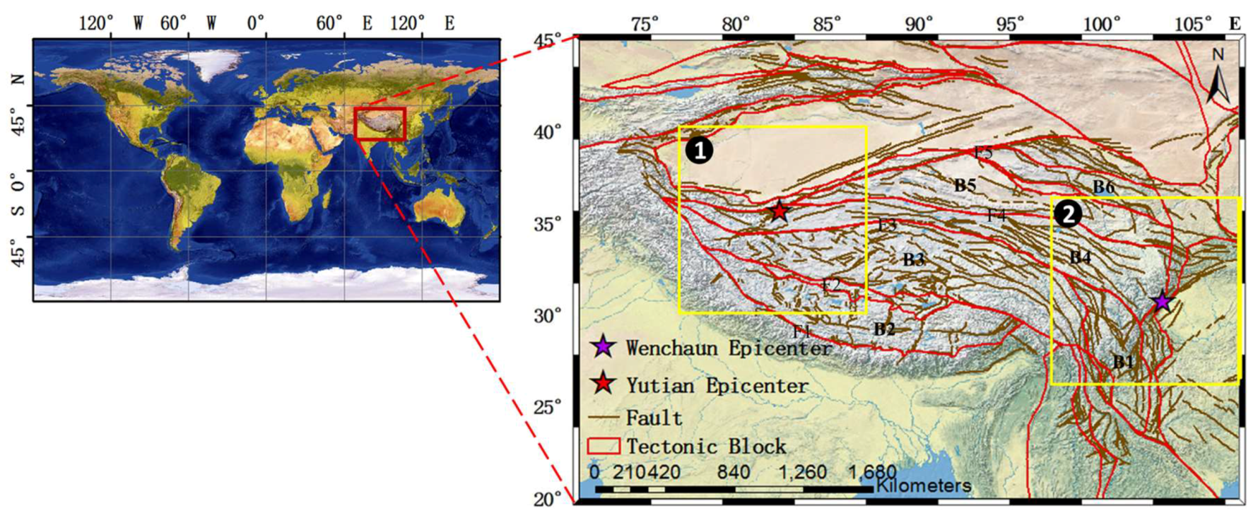
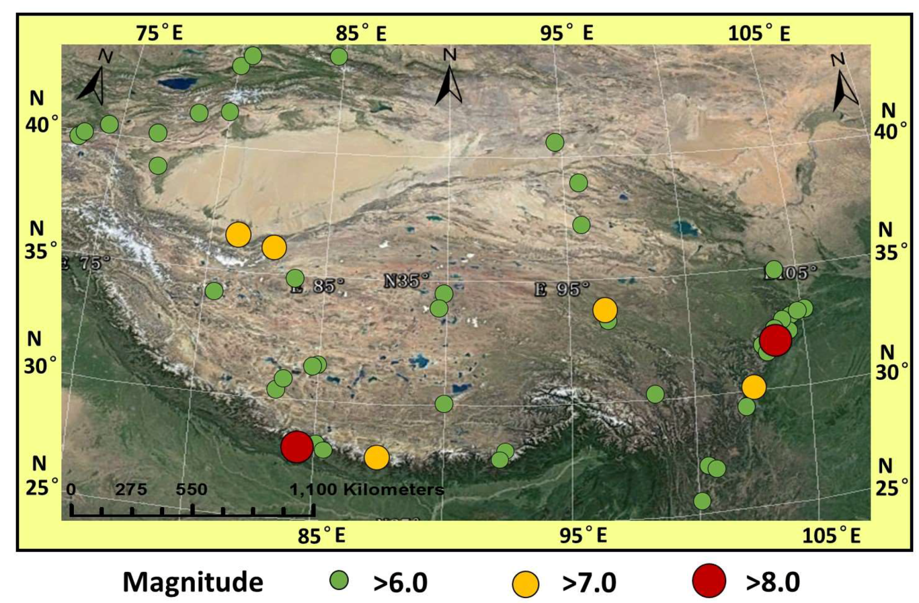
2.1. Study Area and the Two Examined Earthquake Cases

The Qinghai-Tibet Plateau was taken as the study area. As a whole, the Qinghai-Tibet Plateau was actually formed by isostatic mountain building processes beginning in 3.6 Ma, which were accompanied by the isostatic subsidence of the peripheral basins and depressions, and major changes in the topography and environment of the area. A series of pulsating mountain building events occurred at 3.6 Ma, 2.5 Ma, 1.8 to 1.2 Ma, 0.9–0.8 Ma, and 0.15–0.12 Ma, which were associated with the equilibrium of gravity and the isostactic adjustments of the crustal materials. There events led to the formation of a composite orogenic belt in which the originally relatively independent Himalayas, Gangdise, Tanghla, Longmenshan, Kunlun, Altyn Tagh, and Qilian Mountains became unified. The result was the formation of the complete Qinghai-Tibet Plateau with a unified mountain root following the Miocene uplift of the entire plateau [73]. With its very thick continental crust (70 km thickness on average; double the normal thickness of the crust), and the dramatic uplift of the late Pleistoeene period (now with an average elevation of between 4500 and 5000 m), along with its sustained and strong tectonic deformations [74], the Qinghai-Tibet Plateau has become one of the most unique geological areas in the world. It spans across Eurasia, and is an important part of the Alps-Himalayan tectonic belt. The stratum development of the plateau is now complete. The drastic lifting movement is known as the “the roof of the world”, where a series of large-scale and active fault zones have been formed since the Cenozoic. These fault zones include the following: the Himalaya main thrust belt (F1); Karakorum-Jiali fault zone (F2); Mani-Yushu-Xianshuihe fault zone (F3); Kunlun-Maqin fault zone (F4); Altyn-Haiyuan fault zone (F5); and the Jinshajiang-Honghe fault zone (F6), from the south to the north. These six main fault zones divide the Tibetan Plateau into six different active blocks as follows: The Chuandian (B1); Lasa (B2); Qiangtang (B3); Bayankala (B4); Chaidamu (B5); and Qilian (B6) [69], as shown in Figure 1.
The Tibetan Plateau is a very important seismically active region which is known for its high incidence level of earthquakes due to its special tectonic region, i.e., locating the convergence region where the Indian Plate extrudes the Eurasian plate from south to north. Most of the tectonic activity occurs on the boundaries of the blocks [75,76]. Earthquakes are the results of abrupt releases of accumulated strain energy that reaches the threshold of strength of the earth’s crust. The boundaries of tectonic blocks are the locations of the most discontinuous deformation and highest gradient of stress accumulation, thus they are the most likely places for strain energy accumulation and releases, and in turn, devastating earthquakes, to occur [75,76]. Previous research indicated that the mechanisms of precursory anomalies can be attributed to degassing from rocks under stress, and the participation of ground water or to p-hole activation in the stressed rock volume and their further recombination at the rock-air interface, especially at the boundaries of active tectonic zone [3,9,23,37,44,45,46,47,48,49,50,51,52,53,54,55,56], thus more TIR anomalies occurred along the tectonic zone [2,8,21,43]. It is well-known that the Tibetan Plateau is made up of the several important second level active tectonic blocks, detailed in Figure 1. Therefore, the area has been hit by many major earthquakes. Only within this territorial region of China, there were nearly 50 shallow earthquakes (focal depth not more than 20 km) with magnitudes greater than Ms 6.0 during the period examined in this study (2003 to 2015, illustrated in Figure 2). Among these, the earthquakes with magnitudes larger than Ms 7.0 consisted of the Ms 8.0 Wenchuan earthquake of 2008; the Ms 7.3 Yushu earthquake of 2010; the Ms 7.0 Yaan earthquake of 2013; and the Ms 7.3 Yutian earthquake which occurred in 2014. These earthquake events caused enormous economic losses and casualties.
On 12 May 2008, at 14:28 local time (06:28 UTC), the devastating Ms 8.0 Wenchuan (Sichuan, China) earthquake ruptured the Longmen Shan fault zone on the eastern edge of China’s Tibetan Plateau (illustrated in the yellow square box labelled 2 in Figure 1) [77]. The main earthquake event was followed by thousands of aftershocks. Among these, 53 reached or exceeded Mw 5.0. This major earthquake caused extreme damages that extended almost 300 km along the Longmen Shan and its adjacent area. A large number of landslides, debris flows, surface fractures, and dammed lakes were observed. Overall, more than 80,000 fatalities were reported. This catastrophic event was one of the deadliest earthquakes in China during the past few centuries.
On 12 February 2014, at 17:19 local time (09:19 UTC), a significant Ms 7.3 Yutian (Xinjiang, China) earthquake occurred in the Altyn-Haiyuan fault zone of the northwest edge of China’s Tibetan Plateau (represented by the yellow square box labelled 1 in Figure 1). The epicenter was located at 36.1°N, 82.5°E, and the depth of the hypocenter of 12 km. This major earthquake event was followed by 739 aftershocks, one of which reached Ms 5.0, and ten reached or exceeded Ms 4.0. As a result of this major disaster, more than 455,000 people became homeless; 68,340 houses were toppled; 11,515 domestic animals were killed; 497 bridges were badly damaged; and 113 landslide events occurred.

2.2. Remotely Sensing Data

The LST is an important index for evaluating the heat balance, which represents a collective outcome of the tectonic activities of the deep Earth’s crust. Also, the terrain and land cover and meteorological activities are known to be important indexes. Therefore, this study adopted the LST to measure tectonic activities. The data used in this study were the synthetic LST datasets with the average surface temperatures of eight days (MOD11A2 Version 5 (V5) of MODIS) provided by NASA, with a 1 km spatial resolution. This V5 product was a significant improvement over past versions. In this experiment, in order to weaken the influences of solar radiation and local variations due to cloud cover or shadows during the day-time hours, the data observed at night were used. In addition, since the MOD11A2 was one of the mature LST products, there was no need to implement atmosphere corrections [66]. The detailed information regarding the data set is summarized in Table 1. The original images of the MOD11A2 are shown in Figure 3 according to the time sequence. Figure 3 shows that the original LST of the MOD11A2 were noticeably dominated by solar radiation and terrain, and exhibited very distinct seasonal characteristics. Therefore, for extracting out the TIR anomalies closely related to tectonic activities, the influences of atectonic factors must be removed from the original MODIS LST data and weakened.

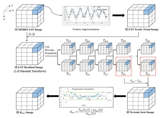
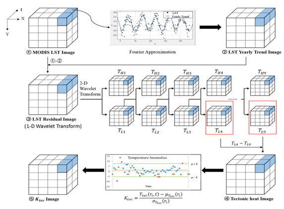
2.3. Introduction of the New Algorithm

The objective of the developed algorithm was to extract the tectonic activities information by filtering or weakening the impact of the atectonic factors (solar radiation, atmospheric disturbances, and human activities. It is widely known that solar radiation is the first and foremost factor which affects the land surface temperature field. It has been regarded as a type of stable annual periodic signal that has observable seasonal fluctuating properties. In addition, the influences of air masses and human activities (urban heat islands) should not be ignored. In accordance with the spatio-temporal scale characteristics of the various interference factors, this study proposed a new algorithm (TTIA) to characterize the tectonic TIR anomalies. The process was introduced in detail as follows:
Step (1)
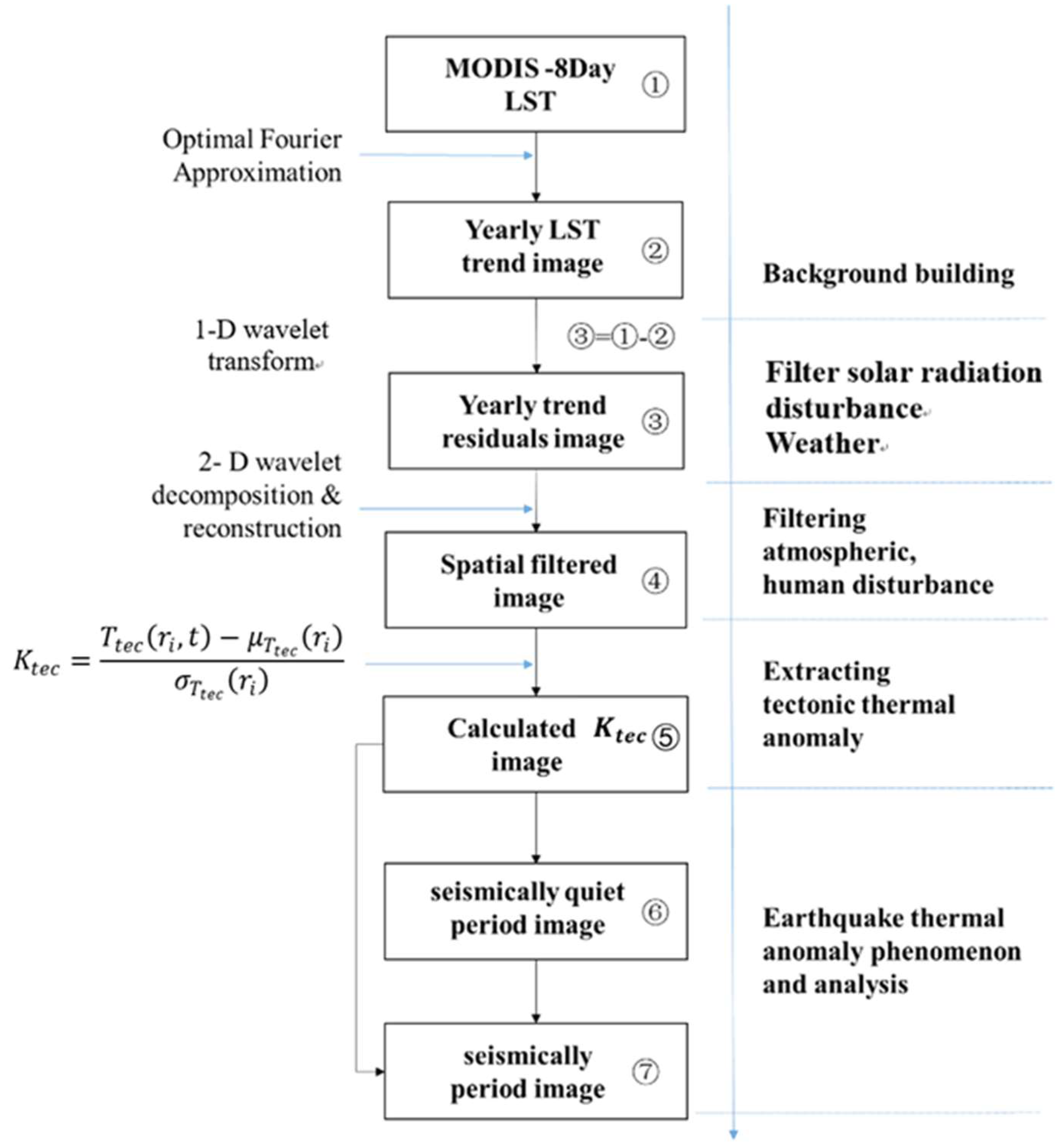
Constructing the LST background field and calculating the residuals: The annual trend values were extracted from the sequential LST data, such as the temperature background field, using a harmonic analysis fitted curve method. The detailed introduction on this step is shown in Section 2.3.1. The fitting residual error image (shown in Step ③ of Figure 4) filtered the solar radiation influence and climate change. We then applied a 1-D wavelet transform, and by means of deleting the first order high frequency of wavelet transform, the effect of the short-term meteorological factors could be removed. However, it still consisted of disturbances in the atmosphere and human activities.
Step (2)
Spatial filtering to weaken the impacts of the atmosphere and human activities (urban heat island): It was considered in this study that the air masses and urban heat islands did indeed have evident influences on the surface temperature field. Therefore, these disturbance factors needed to be removed or weakened. The spatial scales dominated by these two factors were profoundly different. Generally speaking, an air mass can cover hundreds to thousands of km. However, the influence range of the heat islands only measure tens of km [78]. Therefore, a 2-D wavelet transform technique was used in this study to filter the disturbance factors, and extract the tectonic thermal information. A detailed introduction to this is shown in Section 2.3.2.
Step (3)
Presenting the tectonic thermal anomalies information by calculating the value image (shown in ⑤ of Figure 4): Further details of this calculation process are shown in Section 2.3.3.
The above steps were the core parts of this study’s proposed new algorithm, and the process is vividly illustrated in Figure 5.

2.3.1. Construction of the LST Background Field and Calculation of the Residuals

First of all, this study ranked the pixels according to their temporal sequence. Then, a yearly trend value was extracted as the background field by approximating the curve of the LST over a period of 13 years (2003 to 2015). A key point of this process was that all the observed values were regarded as a whole, and a new approximation function was obtained [79,80,81]. A least squares criterion was used to build the new function as follows:
Least squares approximation
By assuming that the known function f ( x ) was defined in the space [ a , b ] , then ρ ( x ) 0 . Where ρ ( x ) is a weight function that is not identical to zero. Also, by assuming that the norm of f ( x ) exists, and that the inner product space is L 2 [ a , b ] , then the norm of f ( x ) can be obtained using Equation (1) [82] as follows:
f ( x ) 2 = a b ρ ( x ) f 2 ( x ) d x
The nature of the optimal approximation in L 2 is that, for any f ( x ) ( a , b ) , function φ ( x ) should be looked for on the basis space M = { φ 1 , φ 2 , , φ n } as follows:
φ ( x ) = i = 1 n c i φ i
which is subject to the following:
a b ρ ( x ) [ f ( x ) φ ( x ) ] 2 d x min
Equation (3) indicated that the square of the error function reached a minimum value after solving the integral. Therefore, φ ( x ) can be referred to as the optimal square approximation of f ( x ) .
Optimal Fourier approximation
When the function to be approximated is periodic, or the primitive function is too complex, then the primitive function has to be approximated using discretization processing. In this study’s case, this step was performed using a Fourier approximation. By letting M be made up of trigonometric functions (sine or cosine functions) [83,84], then φ ( x ) will be the optimal Fourier approximation of φ ( x ) .
Extraction of the LST’s yearly trend
In this study, by taking a pixel as an example, and building a Fourier approximation function as described in Equation (4), a fitting process for the discrete sequence of the LST values in the pixel could then be performed:
y = i = 1 m [ a i sin ( ω i t + b i ) + c i cos ( ω i t + b i ) ] + ε
where i = 1, 2, …, m, and 2m is the number of harmonic; y represents the approximate values; t is the specific moment in a time sequence; a i denotes the amplitude of the i t h sine harmonic; b i is the phase of the i t h harmonic; c i represents the amplitude of the i t h cosine harmonic; ω i is the phase of the i t h harmonic; and ε is the fitting error.
By considering the annual and diurnal changes of the LST, two types of harmonics with different frequencies were chosen to approximate the time series. One type with a 0 frequency indicated the average of LST, and that there was no phase. Meanwhile, the other type had a period of eight days, which represented the short-term variations of the LST.
As indicated above, the principle of the least square method was considered in the calculation of the variables during the approximation process, as described in Equation (5). The values of ai, bi, and c i could be obtained by computing derivatives as follows:
ε 2 = j = 1 n { y j i = 1 m [ a i sin ( ω i t + b i ) + c i cos ( ω i t + b i ) ] } 2

2.3.2. Tectonic Thermal Signal Extraction by Spatial Two-Dimensional Wavelet Filtering for the Purpose of Weakening the Disturbances of the Atmospheric and Human Activities

Although the LST fitting residuals had filtered out the main disturbances of the solar radiation, it still contained the disturbances resulting from the atmosphere and human activities. It was believed that separating the two types of thermal information from the residual images would allow for improvements in the extraction of the thermal information related to the tectonic activities. After considering the spatial affected scope of the air masses and human activities, this study applied the different features between them to achieve the signal separation using a 2-D wavelet transform.
Theory of the 2-D wavelet transform
2-D continuous wavelet transform
The 2-D continuous wavelet transform was defined as follows [7]:
W f ( a , b x , b y ) = f ( x , y ) Ψ a , b x , b y ( x , y ) d x d y
Ψ a , b x , b y ( x , y ) = 1 a Ψ ( x b x a , y b y a )
Its inverse was given by Equation (8):
f ( x , y ) = 1 C Ψ 0 + + + W f ( a , b x , b y ) Ψ a , b x , b y ( x , y ) d b x d b y d a a 3
where a is a scaling transformation parameter; and b is a displacement transformation parameter. When the value varied, the wavelet function changed, which corresponded to the elongation and contraction. That is to say, when a < 1 , Ψ ( x , y ) was elongated; and when a > 1 , Ψ ( x , y ) had contracted. When the value of b changed, the wavelet function exhibited a displacement.
2-D discrete wavelet transform
Due to the computational complexity of the continuous wavelet transform in terms of the continuous values a , a 2-D discrete wavelet transform is often used to conduct the wavelet transformation of a digital image. In this study, the 2-D discrete wavelet transform was defined as follows [83]:
Ψ m , n ( t ) = 1 a 0 m Ψ ( t n b 0 a 0 m a 0 m ) = a 0 m 2 Ψ ( a 0 m t n b 0 )
where m , n are the integer, a 0 1 and b 0 0 . The corresponding discrete wavelet transform can then be defined as follows:
f , Ψ m , n = a 0 m 2 + f ( t ) Ψ ( a 0 m t n b 0 ) d t
The reconstruction process was the inverse process of the 2-D discrete wavelet image decomposition. The digital images, which had met certain requirements, could be reconstituted through controlling the high and low frequency components of the decomposition process of the wavelet transform.
Tectonic thermal infrared signal extraction based on a 2-D wavelet transform
Except the solar radiation, among the influencing factors that dominate the land surface temperature, atmospheric air mass and human activities are two important and ought not to be missed factors [84]. Generally speaking, a distributed air mass extends up to a large scope at a horizontal direction with a homogeneous temperature and humidity characterization [85]. In terms of the thermal property, an air mass can be divided into a cold air mass and warm air mass [86]. The arrival of an air mass with certain thermodynamic properties can vary the land surface temperature. Therefore, the influence of an air mass on the land surface temperature must be removed [86]. According to the field of meteorology and physical geography, an air mass can cover a range of several hundred to several thousands of km. In this study, in order to facilitate the calculation process, the temperature components with ranges of more than 1000 km were taken as the contribution of the atmospheric air mass [84,85,86,87]. In regard to the disturbances caused by human activities, such as the urban heat island effect, the influence ranges were roughly tens of km (the length of the diameter of a city) [88,89]. Therefore, approximately 30 km was chosen in this study as the influence range of the human activities [84,89]. Then, using a wavelet transform technique, these two types of disturbances could be weakened to a certain degree.
To be more specific, since the spatial resolution of the MODIS LST dataset used in this study was 1 km, and considering the fact that the sampling of the wavelet transform abided by the geometry power of two, the thermal infrared signal was able to extract more information related to the tectonic activities by using the 2-D wavelet transform from the residual images. This was accomplished by weakening the influences of the solar radiation, atmospheric air masses, and human activities. As a result, it could be defined as T t e c , and the calculation formula is given in Equation (11):
T t e c = T L 4 T L 9
where T L 4 represents the LST, which was extracted from the low frequency signal of the 2-D wavelet transform in the 4th scale (corresponding to a 32 km resolution) of the residual images; T L 9   is the LST extracted from the low frequency signal of the 2-D wavelet transform in the 9th scale (corresponding to a 1024 km resolution) of the residual images.

2.3.3. Expressions of the Tectonic Thermal Infrared Anomalies
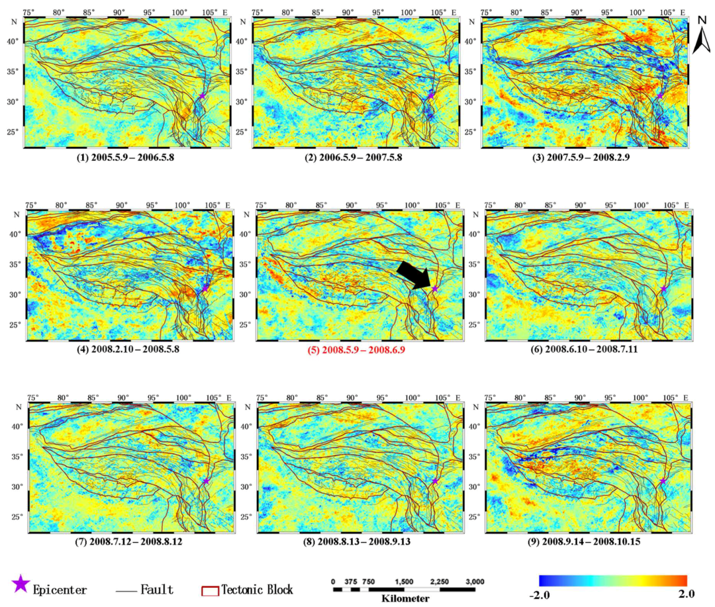
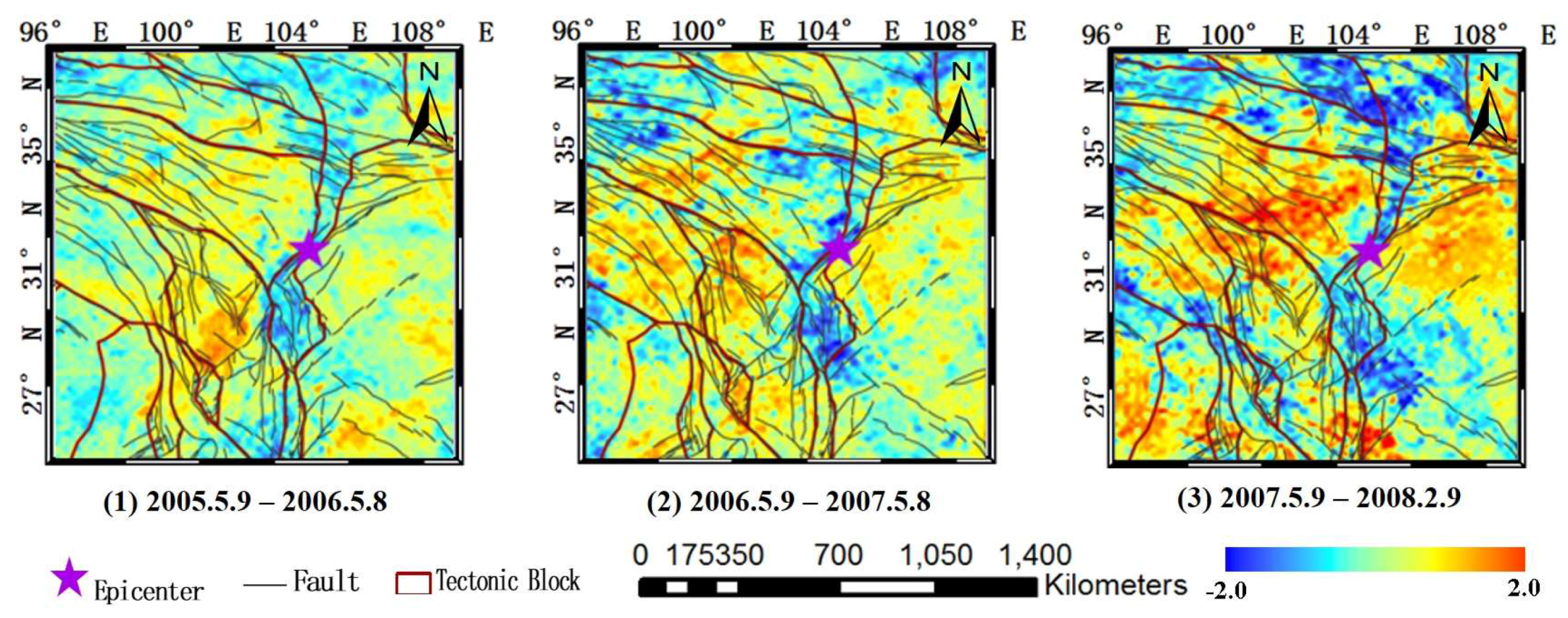
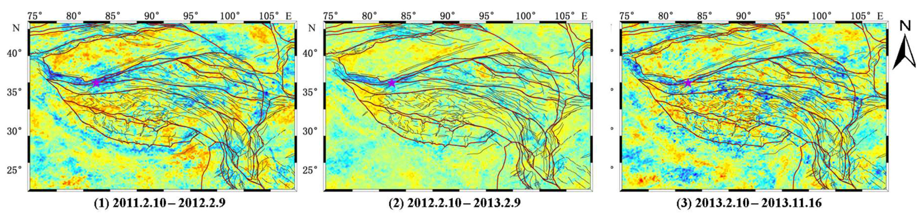
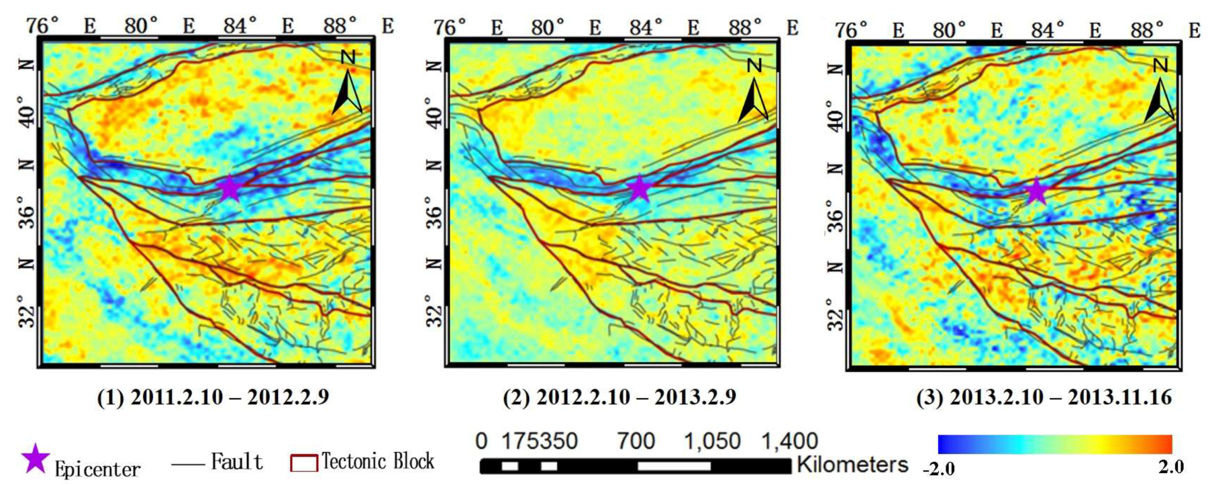
k σ ”rule and offset index K t e c
In this study, the “ k σ ”rule was used to determine the signals of the thermal anomalies. The “ k σ ” principle was proposed initially by Wright in 1884 [90,91,92,93]. This simple and basic principle is as follows:
| x i x ¯ | k σ
where x and σ are the mean and standard deviation of the result x, respectively. Here the “ k σ ” rule is introduced to characterize the variation of land surface temperature observations around their mean, where k refers to the zoom multiples of standard deviation σ. When the result x meets the above formula, then it can be defined as an anomaly signal, as illustrated in Figure 6.
The effective thermal infrared signal values T t e c were achieved using Equation (11). Then, the thermal anomalies were extracted through calculating the offset index K t e c according to Equation (13). In fact, K t e c is just the embodiment of the k value in the formula (12). The introduction of K t e c   aims to characterize the variation of land surface temperature observations around their mean. Meanwhile, K t e c can also be perceived as zoom multiples of standard deviation σ T t e c ( r i ) .
K t e c =   T t e c ( r i , t ) μ T t e c ( r i ) σ T t e c ( r i )
where r i denotes the location of pixel i on the remote sensing image, with the abscissa and ordinate ( x i , y i ) ; t represents the time of the acquisition of the satellite image, with t τ , where τ defines the homogeneous domain of the satellite imagery collected in the same time-slot (hour) of the day and period (month) of the year; T t e c is the effective thermal infrared signal; and μ T t e c and σ T t e c are the mean value and standard deviation of the T t e c in the same time-slot, respectively. It is worth noting that although equation 13 has a similar formation to the RST method, which was proposed by Tramutoli 1998 (RAT) [25], Tramutoli 2005 (RST) [38] and applied by Lisi et al. 2015 [42], who have used in the same way the reference fields of mean and standard deviation; nevertheless, in equation 13, T t e c has a distinct meaning from T in the RST method. Here T t e c has filtered the influence of air mass and human activities by a 2-D wavelet transformation, therefore μ T t e c , and   σ T t e c in the Equation (13) has distinct T t e c basis, compared with the μ and   σ in the RST method.

3. Results

In the study results, two important observation scales were adopted to describe the TIR anomalies in tectonic activities based on the proposed method. The first method was the whole Qinghai-Tibet Plateau scale, while the other was the earthquake generating fault zone scale. The Tibet Plateau contributes to observing the TIR in tectonic activities on a large scale, and to understanding the TIR anomalies evolution of the pregnant process of earthquakes before a large earthquake event. It is well known that earthquakes are the manifestations of abrupt huge energy releases that are directly caused by tectonic activities. Since earthquakes are known to be highly related to tectonic activities, it can be deduced that the relevant precursor signals of earthquakes should be evidently strongly correlated with tectonic structures. We chose two large earthquake events that had occurred on the Tibet Plateau, based on the consideration that before the large earthquakes events occurred, the TIR in the tectonic activities often varied significantly and observably, which makes it more convenient for us to observe the spatio-temporal evolution characterization of TIR and validate the new algorithm.
The period in the red typeface in Figure 7 indicates the co-seismic period. The thermal anomaly images shown in Figure 7(1)–(9) were calculated according to the following steps: Step (1) The calculation of the K t e c values was performed using Formula (12), which indicated the tectonic thermal anomaly; Step (2) The abnormal periods were identified, which needed to meet the request that K m e a n μ + σ . In this study, K m e a n is the spatial mean of the K t e c value image in a period; μ is the mean of the K t e c value images in the multi-periods; and σ is the variance of the K t e c value images in the multi-periods; Step (3) All of the selected images were overlaid by Step (2), and the average value of the image was calculated; Step (4) The differences in the value image were calculated between the average value image calculated by Step (3), and the K t e c mean value image of the aseismic periods (without the occurrence of large earthquakes).
Figure 7 illustrates the fact that the spatial form of the TTIA-based TIR anomalies corresponded well in this study to the tectonic zone distributions, which potentially provide evidence that judging the extracted TIR anomalies signals based on the new method is reasonable. This is particularly evident in Figure 7(3). The noticeable characteristics of the spatial distribution of most of the TIR anomalies from east to west, along with the major faults zones of the entire Tibetan Plateau, leads us to believe that the proposed TTIA algorithm was able to reflect tectonic activities well, as it can efficiently filter out the majority of the other atectonic disturbance information originating from the impacts of solar radiation, land cover, atmospheric and human activities. Figure 7 displays the evolution history of the TIR anomalies before and after the earthquake events, which was helpful in understanding the seismogenic stages of major earthquakes. It is well known that every earthquake has a long seismogenic stage, which may range from several decades to hundreds or even thousands of years. Generally speaking, the larger magnitude earthquakes have longer seismogenic stages. In this study, the TIR anomalies evolutions were observed and analyzed, with special emphasis on the period from the three-year pre-seismic stage to the breaking out stage of the earthquakes, in order to grasp the evolutionary characteristics of the TIR anomalies signals during the latter seismogenic stage. Figure 7(1)–(3) illustrate the developing processes of the TIR anomalies from May of 2005 to February of 2008 (prior to the Wenchuan earthquake) over the entire Tibetan Plateau region. The value of the TIR anomalies can be obviously seen as gradually rising during the period from three years to three months prior to the Wenchuan event. Also, in that period the K t e c value of the east was clearly higher than that of the west on the plateau. According to the theory of the relationship between the heat and stress in laboratory testing (temperature-rise corresponding to extrusion stress), it was deduced that the surrounding rock in the active tectonic block was increasingly extruded along the direction from east to west. This was confirmed by the observed GPS results. Until February 9th, 2008 (approximately three months before the Wenchuan earthquake), the temperature in the area had been reaching its highest value, as shown in Figure 7(3)). This was the first observed important temperature-rise stage. Then, after passing the stage of the highest value of the TIR anomalies, the temperature was observed to slightly decline, as shown in Figure 7(4). Soon after, the devastating earthquake event occurred, after which the TIR anomalies fell to a relatively low level, as detailed in Figure 7(6)–(8).
Figure 8 shows the enlarged images from Figure 7. The TIR anomalies were derived by means of the proposed algorithm in the Lonmenshan fault zone where the Ms 8.0 Wenchuan earthquake occurred. It can be seen that the TIR anomalies based on the TTIA method are in high correspondence with the tectonic line.
Figure 9 illustrates the moving tendency of the intensity centroid in the K t e c evolution process prior to the Wenchuan earthquake event. The green, yellow, and red points denote 2 to 3 years, 1 to 2 years, and 3 months to 1 year prior to the earthquake, respectively. The centroid apparently had gradually moved from the left to the right of the TIR anomalies image, and toward the epicenter of the Wenchuan earthquake. In reality, this was a significant signal, and important information was obtained that revealed that the eastern region over the Tibetan Plateau seemed to be facing a higher threat than the western region, which will potentially contribute to future estimations of dangerous regions where earthquakes might occur.
In regard to the Yutian earthquake, the evolution trend of the K t e c can be seen in Figure 10. As can be seen in the figure, the value of K t e c was not only consistently distributed along the trend of the tectonic faults, but also the K t e c of the surrounding rock in the tectonic block was observed to steadily rise until the highest value was reached. At that time, the value of the K t e c of the western region was higher than that of the eastern region.
Throughout the entire process of the K t e c evolution over the Tibetan Plateau in both of the major earthquake cases examined in this study, it was found that prior to the earthquake events, the spatial distributions of K t e c were almost entirely arranged along the significant fault zones. Also, the majority were extended along an east-west direction, which confirmed that the proposed TTIA algorithm could accurately reflect the tectonic activities. Therefore, it was concluded that the TTIA-based K t e c could be regarded as a precursor indicator for outlining potentially dangerous regions where major earthquakes may occur in the future.
Figure 11 shows the TIR anomalies based on the TTIA method in the Altyn-Haiyuan fault zone where the Ms 7.3 Yutian earthquake occurred. It can also be clearly seen that the TIR anomalies are in high correspondence with the tectonic line.
Figure 12 illustrates the moving tendency of the intensity centroid in the K t e c evolution process prior to the Yutian earthquake event. The green, yellow, and red points represent the same as in Figure 9. Overall, it was observed that the intensity centroid of the K t e c hovered around the western region of the plateau. In particular, in the entire energy of the anomalies with K t e c ≥ 1.0 detailed in Figure 12a, the centroid (indicated by the yellow point) almost coincided with the epicenter of the Yutian earthquake. The calculated intensity centroid potentially indicated that the western region of the plateau seemed more dangerous than the eastern region. These findings were very valuable signals, which provided supplementary information for outlining dangerous regions, and served as early warning signs of the earthquake events.
In this study result, another observable scale is the earthquake generating fault zone. The spatio-temporal evolution of the TIR anomalies in tectonic activities with the TTIA algorithm in the fault zone scale (Longmenshan fault zone and Altyn fault zone) are shown in Figure 13, Figure 14, Figure 15 and Figure 16. The following observations can be made: (1) Before the great earthquake, the fluctuations of the K t e c   value are significantly more volatile than those in an aseismic period, which indicates that the TIR anomalies in tectonic activities in the event year are more active than those in non-event years. (2) In an unperturbed period (when no large earthquake occurs), the K t e c value presents low value features in both the Longmenshan fault zone (shown in Figure 14) and Altyn fault zone (shown in Figure 16). Despite the fact that there are also some high or low K t e c pixels, their distribution still did not present distinct regularity.
Further observing Figure 13, we can observe the fact that during the period of three to six months before the Wenchuan earthquake event, the surrounding rock of the Longmenshan Fault presented an increasing trend in the K t e c , approximately 100 days before the earthquake, and the K t e c of the surrounding rock reached its highest value. Then the K t e c began to decline. On the contrary, during this period, the fault region went through a cold status before the earthquake. Then around three months before the event, the situation changed. The fault region was going through a hot thermal anomaly state, breaking away from the previous cold anomaly state; i.e., the temperature of the fault zone underwent a change process from cold to hot status. After the earthquake, the value of the K t e c in the fault region declined, exhibiting an increasingly discrete state in terms of spatial distribution. A similar phenomenon can be also observed in the Yutian earthquake event which occurred on the Altyn fault on 12 February 2014.
The above mentioned observed phenomenon appears to not be coincidental. In fact, we have investigated the characterization of TIR anomalies in tectonic activities before an earthquake event year via the TTIA method using four earthquake cases of magnitudes greater than Ms 7.0 over the Tibet Plateau since 2003, similar phenomena were observed in each; namely, before the large earthquake, the temperature of the surrounding rock underwent a heating to cooling process, while the temperature of the fault region underwent an inverse process. However, when we investigated earthquakes of magnitude Ms 6.0 or less, we did not observe this kind of very obvious regularity.
The possible explanation for the TIR anomalies in tectonic activities occurring before a large earthquake event is that it is the integration result of the green house air degassing from the Earth’s crust and the stress of rocks. On one hand, green house air is able to warm up the air, thereby leading to three phase changes of water vapor, which can produce the variation of the air temperature. On the other hand, the compression and tension of rocks can result in LST variation through a series of complicated geophysical and geochemical processes.

4. Discussion

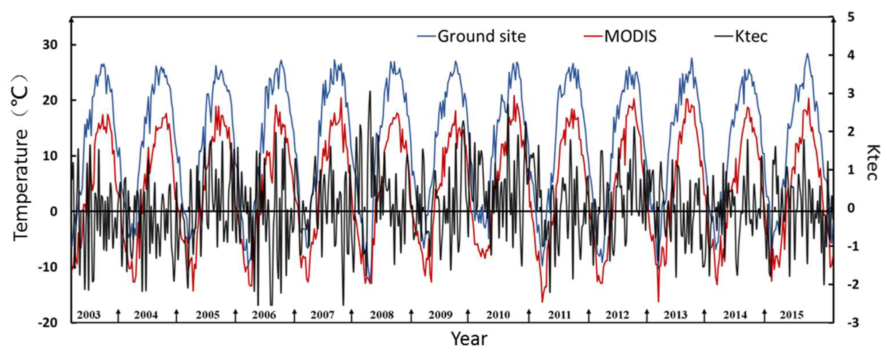
4.1. Comparison of the MOD11A2 LST and Ground Air Temperature Data, TIR Anomalies Value

Figure 17 shows the comparison between the MOD11A2 LST and air temperature observed by the ground site and the TIR anomalies value based on the TTIA method. It can be clearly seen that the MOD11A2 LST data are in high correspondence with the air temperature from the ground site, which can verify the efficiency of the MOD11A2 LST data. Meanwhile, the air temperature observed by the ground site is always higher than the MODIS LST, which can be attributed to the fact that the air temperature data are obtained during the day, while the MODIS LST used in the study are observed at night. The annual variation and very distinct seasonal characteristics of the original MOD11A2 LST data can be clearly observed, and this is the most important disturbance factor influencing the extraction of the tectonic TIR anomaly information. This is the reason for which we must first remove the influences of the solar radiation in the algorithm. Upon closer observation, we can see that the evolution process of the TIR anomalies based on the proposed TTIA algorithm is different from the original MODIS LST and ground air temperature, which indicates that the TTIA method can effectively remove the influence of solar radiation.

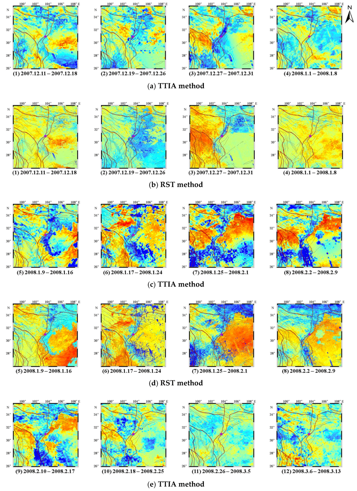
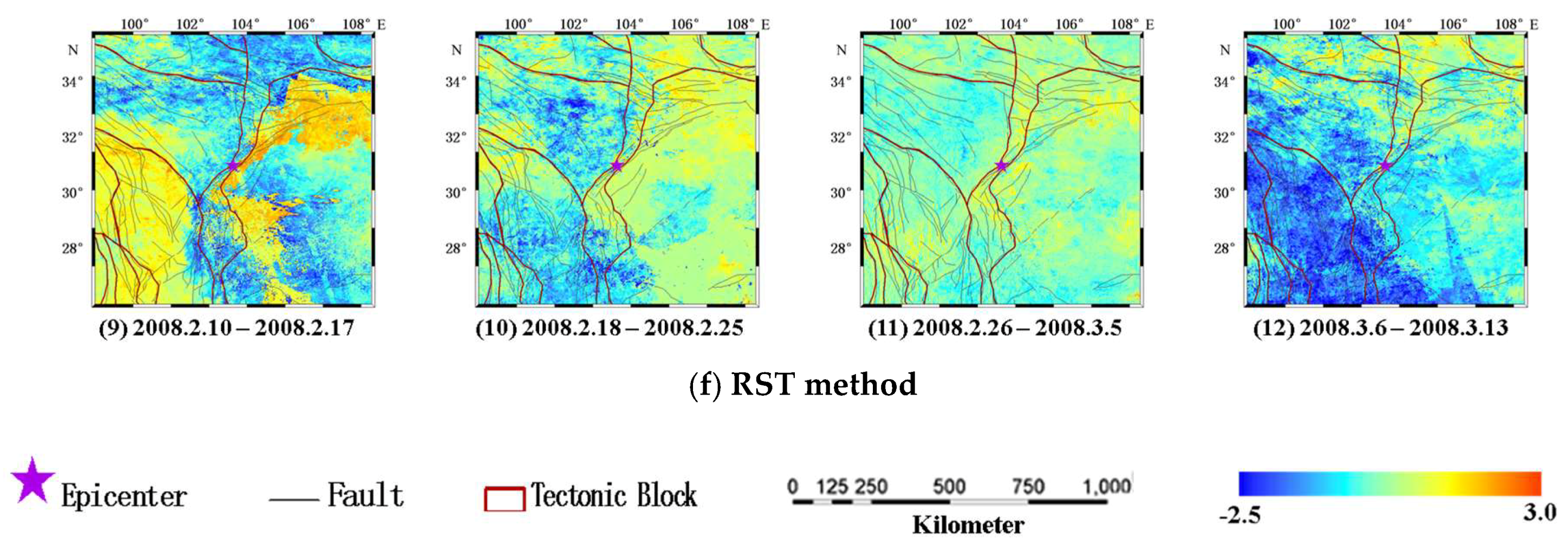
4.2. Comparison of the TTIA and RST Algorithms

The RST method is also an effective TIR anomalies extraction algorithm. It is based on a multi-temporal analysis of the historical data set, which is defined as follows:
Δ T ( r , t ) = Δ T ( r , t ) μ Δ T ( r ) σ Δ T ( r )
where r ( x , y ) represents the location coordinates on a satellite image; t is the time of acquisition of the satellite image at hand, with tτ, where τ defines the homogeneous domain of the satellite imagery collected in the same time-slot (hour) of the day, and the same period (month) of the year; Δ T ( r , t ) denotes the difference between the current ( t = t ) TIR signal value T ( r , t ) at location r , and its spatial average T ( t ) , computed in place on the image at hand, with the cloudy pixels discarded, and only the land pixels considered; μ Δ T ( r ) and σ Δ T ( r ) are the average and standard deviation values of Δ T ( r , t ) , at location r , respectively, computed on cloud-free satellite records belonging to a selected homogeneous data-set ( t τ ).
Although Equation (13) shows a certain similarity to Equation (14) in form, there were evident differences observed between the two. The input of the RST algorithm was the difference values between the LST and the mean value of all of the LST data in a spatial domain observed at the same time, the objective of which was to filter out the weather disturbances. However, the input of the TTIA algorithm was the T t e c , which was more closely related to the tectonic activities, due to the fact that the influences of solar radiation, atmosphere, and human activities had been filtered out.
The experimental results shown in Figure 18 exhibited the spatial distribution at Tibetan Plateau scope of the LST-based TIR anomalies with a contiguous group distribution characterization, rather than extending along the tectonic faults like the TTIA-based TIR anomalies shown in Figure 6. This was the main observed distinct difference between the TTIA and RST methods in regard to reflecting the spatial distribution of TIR anomalies on a large plateau scope. The extracted TIR anomalies space form prompted us to believe that the TTIA method is more sensitive to the tectonic TIR anomalies.
Figure 19 shows the comparison of the spatio-temporal evolution of TIR anomalies extracted by the RST method and TTIA method respectively in the Longmenshan fault region six months to two months before the devastating Ms 8.0 Wenchuan earthquake event of 2008. From Figure 19, the following facts can be clearly observed. The spatial distribution of TIR anomalies based on the RST are roughly similar to those based on the TTIA method, such as in Figure 19a(3),b(3), yet nevertheless there was still some difference in the detailed section in the TIR anomalies between both methods, i.e., the distribution features of the clumps of TIR anomalies were more obvious in the RST method than the TTIA method. In addition, comparing Figure 19c(5–8),d(5–8), we can observe that, although the general distribution of the TIR anomalies was similar, the contrast between the positive TIR anomalies in the surrounding rocks region and negative TIR anomalies in the Longmenshan fault region based on the TTIA method was distinctly stronger than that based on the RST method, which demonstrated that the TTIA method was possibly more sensitive to the tectonic TIR anomalies signal.
The calculated results of TTIA and RST in the Longmenshan Fault zone are presented in a time series, shown as Figure 20 and Figure 21. Each black or red dot indicates the mean value of TIR anomalies throughout the fault zone ( 10 ° × 10 ° ) in a certain 8-day period between 2003 and 2015. In addition, it must be emphasized that the red dots indicate that earthquakes with magnitude between Ms 6.0 to Ms 6.5 took place in the corresponding period. The red arrow shows that an earthquake of magnitude greater than Ms 6.5 occurred. The red solid arrow lines indicate that the earthquakes occurred inside the fault zone. The red dotted arrow lines indicate that the earthquake occurred outside the fault zone, yet the epicenter of the earthquake is close to the fault zone, so that they may have produced a certain impact on the tectonic thermal field in the fault zone.
Comparing Figure 20 and Figure 21, we can observe some significant differences between the two methods: (1) The cluster based on the TTIA algorithm presents a more aggregate distribution trend than that based on the RST algorithm during an unperturbed period. This means that the TTIA algorithm has a lower false warning rate. For example, during the period of 2003 to 2004, when no large earthquake occurred, corresponding with the period marked by Figure 20a, in the region of Longmenshan Fault, all of the K t e c -mean is less than μ + 2σ based on the new algorithm. In contrast, during the same period, there are four occurrences where the K t e c   value exceeded μ + 2σ, with the RST method, as shown in Figure 21, which indicates that the TTIA algorithm has a lower false alarm rate compared with the RST algorithm; (2) During the seismic periods, the warning rate of earthquakes of the TTIA algorithm is higher than that of the RST. For example, in the Longmenshan Fault zone, the Ms 8.0 Wenchuan earthquake broke out on 12 May 2008 and the Ms 7.0 Ya’an earthquake occurred on 20 April 2013. Before these two earthquakes, the K t e c value with the TTIA appeared to be more prominent than the RST, as exhibited in stages (b) and (c) of Figure 20 and Figure 21. Specifically, during the period of one year before the Wenchuan earthquake, there were four instances where the Ktec value exceeded the value of μ + 2σ, based on the TTIA method. However, there were only three instances where Ktec value exceeded the value of μ + 2σ, as shown based on the RST method. Similarly, one year before the Ya’an earthquake, there were four instances where the Ktec value exceeded μ + 2σ, as shown by the TTIA method. In contrast, the Ktec value did not exceed μ + 2σ, as shown by the RST method.

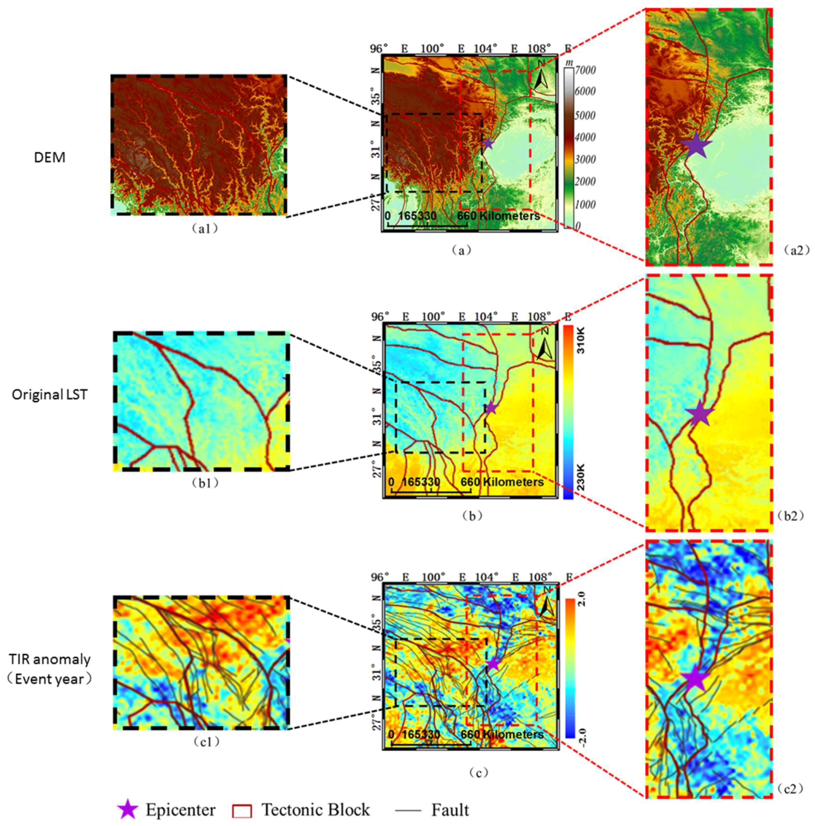
4.3. Comparison of TIR Anomalies Based on TTIA and Tectonic Lineations, Topographic Effect

Figure 22 shows the DEM (Digital Elevation Model) data, original MODIS LST data and the TIR anomalies based on TTIA algorithm. Comparing the Figure 22(a1),(b1), it can be seen that original landsurface temperature is mainly controlled by the topography because there is a good correspondence between the terrain of valley and high landsurface temperature. Figure 22(a2),(b2) also shows a similar pattern. This indicates that the topography is the important leading factor of the original landsurface temperature. Figure 22(c1),(c2) presented the TIR anomalies extracted by the TTIA algorithm. It can be obviously seen that there is no correspondence between the TTIA-based TIR anomalies and the terrain, which demonstrates that the TTIA algorithm is able to remove the influence of the terrain, and simultaneously highlight the active tectonic lineations characteristic. Particularly, comparing Figure 22(a2),(c2), it can be easily seen that there are very distinct difference between the value of the DEM and TIR anomalies in the Longmenshan fault zone, which indicates once more that the TTIA algorithm is able to remove the influence of the topographic effect of ridges/valley in such a mountainous region and reflect the tectonic features well.
Figure 23 shows the DEM data, original MODIS LST data, TIR anomalies based on the TTIA algorithm in the event year and the undisturbance year (no Ms ≥ 5 earthquakes), GPS displacement data, and tectonic fault vector data over the Tibet-plateau. Comparing Figure 23(A1),(B1), and Figure 23(A2),(B2), same rule can be obtained; i.e., the original landsurface temperature on the whole Tibet plateau is controlled by the topography. The black arrows in Figure 23(C1) indicate the vector of the GPS displacement. Observing the GPS displacement, we can know that the Karakorum-Jiali fault zone (shown in Figure 1 with F2) is a active tectonic zone. Meanwhile the TIR anomalies based on the TTIA algorithm present a very obvious distribution characteristic along the active tectonic zone no matter the event year or the undisturbance year. Previous studies demonstrate that the TIR anomalies correspond with main tectonic lines [2,8,21,43], due to the fact that the active tectonic lines made up of the faults are often the channel of greenhouse gases, such as CO2, NH4 and so on, degassing from rocks under stress, and as well as the participation of ground water as a possible cause for generation of TIR anomalies or p-hole activation in the stressed rock volume and their further recombination at the rock-air interface [9,23,50,51,52,53,54,55,56]. The study results demonstrate that the TTIA algorithm is an effective algorithm to extract the TIR anomalies ralated to the tectonic zone. However, further comparing the Figure 23(C1),(D1), we can find that in an event year, the TIR anomalies are more dramatic than that in an undisturbance year.
In a word, through the comparison of the TTIA algorithm-based TIR anomalies and original MODIS LST data, DEM data, GPS displacement data and as well as the active tectonic lines extension direction, we can know that the TTIA algorithm can reduce the disturbance of the atectonic factors, such as solar radiation, air circulation, human activities, and terrain. The study result shows that the TTIA algorithm is effective for the characterization of thermal infrared anomalies in tectonic activities. Moreover, the dangerous region which has high possibility to meet an impending earthquake can be sketched by calculating the gentroid of the TIR anomalies based on this TTIA algorithm. It should be noted that the outline of earthquake danger zone based only on TIR anomalies is not enough. Other pre-earthquake anomalies such as the electromagnetic anomalies in the atmospheric ionosphere, extracted by the Swarm satellite [93] and DEMETER satellite [94] should been incorporated.

5. Conclusions

In this study, a novel TTIA (tectonic thermal infrared anomalies) method was proposed to characterize earthquake TIR anomalies. The Tibetan Plateau was chosen as the study area. Then, using the MODIS land surface temperature (LST) products MOD11A2 via the proposed method, this study observed the spatio-temporal evolution of the TIR anomalies over the plateau from 2003 to 2015. A method that combined the typical earthquake cases, and analyzed the TIR anomalies signals of the pre-seismic, co-seismic, and post-seismic periods, was implemented, which allowed for a deeper understanding of the earthquakes’ TIR anomalies features. The TIR anomalies rule at a plateau scale and fault zone scale was examined prior to the onset of the major earthquake events in the area. Then, after analyzing this study’s experimental results, the following conclusions were drawn:
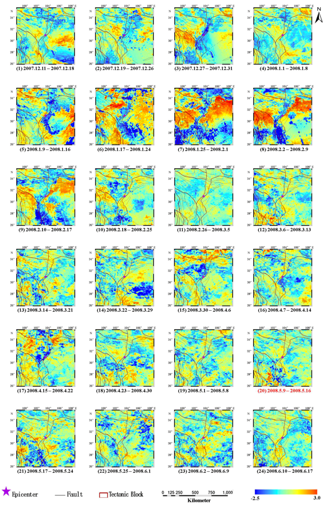
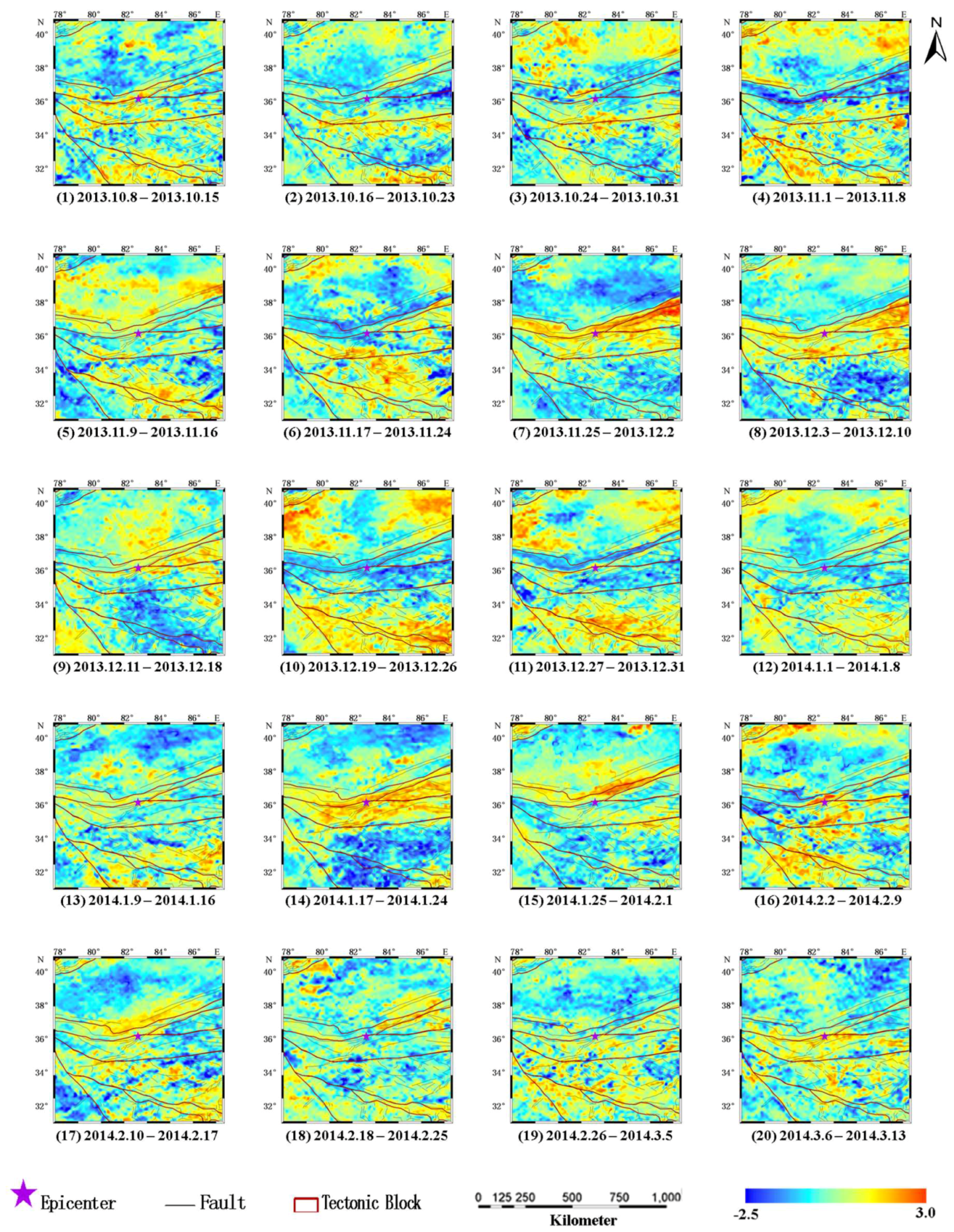
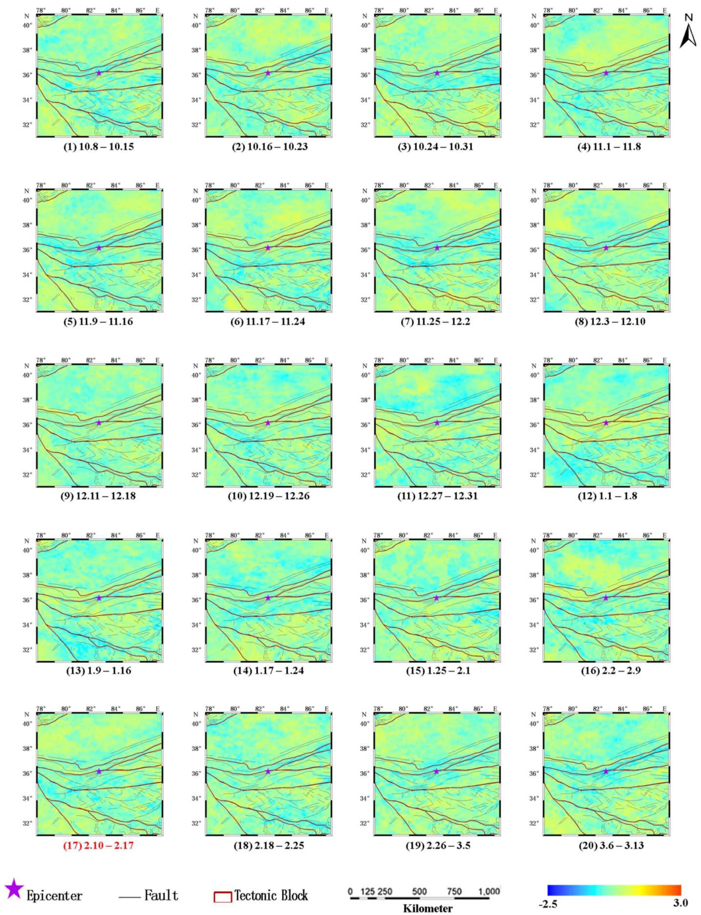
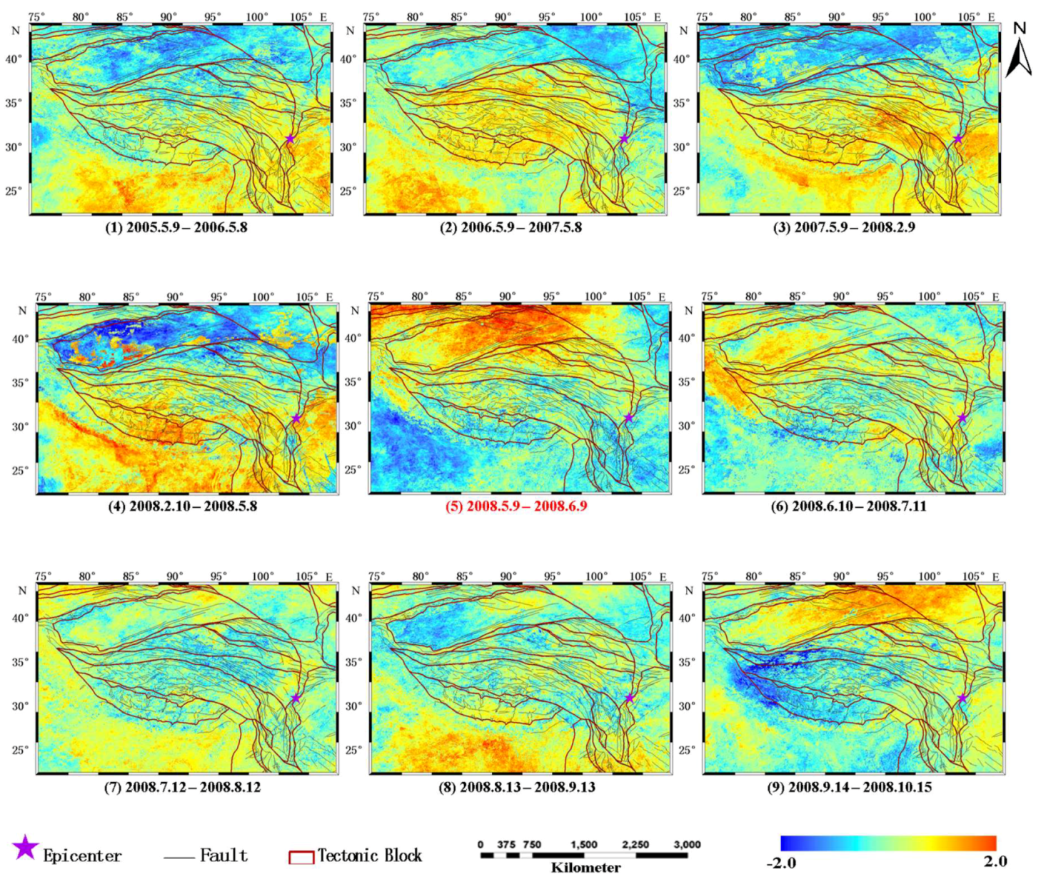
  • The obtained TIR anomalies based on the new algorithm showed an obvious spatial distribution characteristic along the main faults on the plateau. Therefore, it can be proved that the proposed algorithm had distinctive advantages in removing or weakening the disturbances of the atectonic factors, and was therefore very effective in extracting the tectonic TIR anomalies signals.
  • The seismogenic zone was found to be a more effective observation scope for the deeper understanding of the mid- and short-term seismogenic and crust stress change processes.
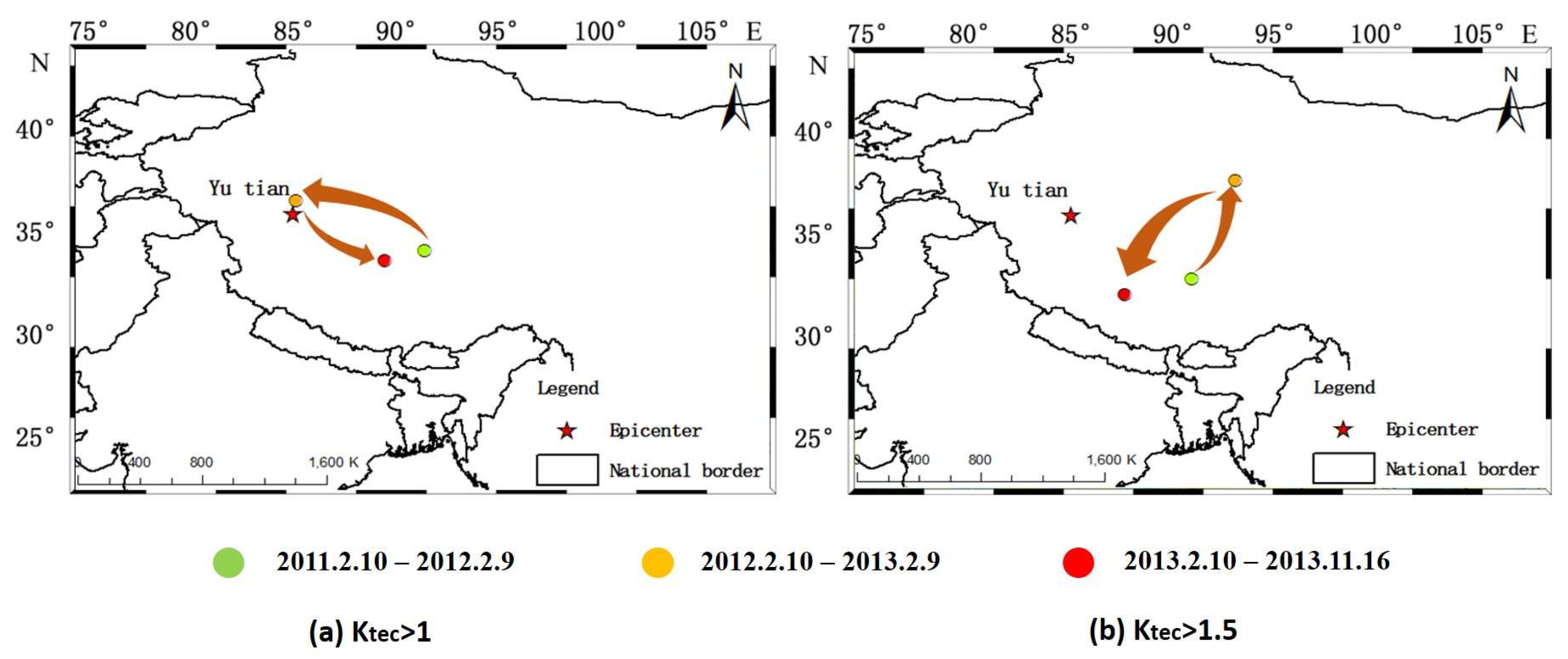
  • The movement trace of the centroid of the TIR anomalies over the entire plateau was helpful in judging the approximate dangerous tectonic regions where major earthquakes may occur in the future.
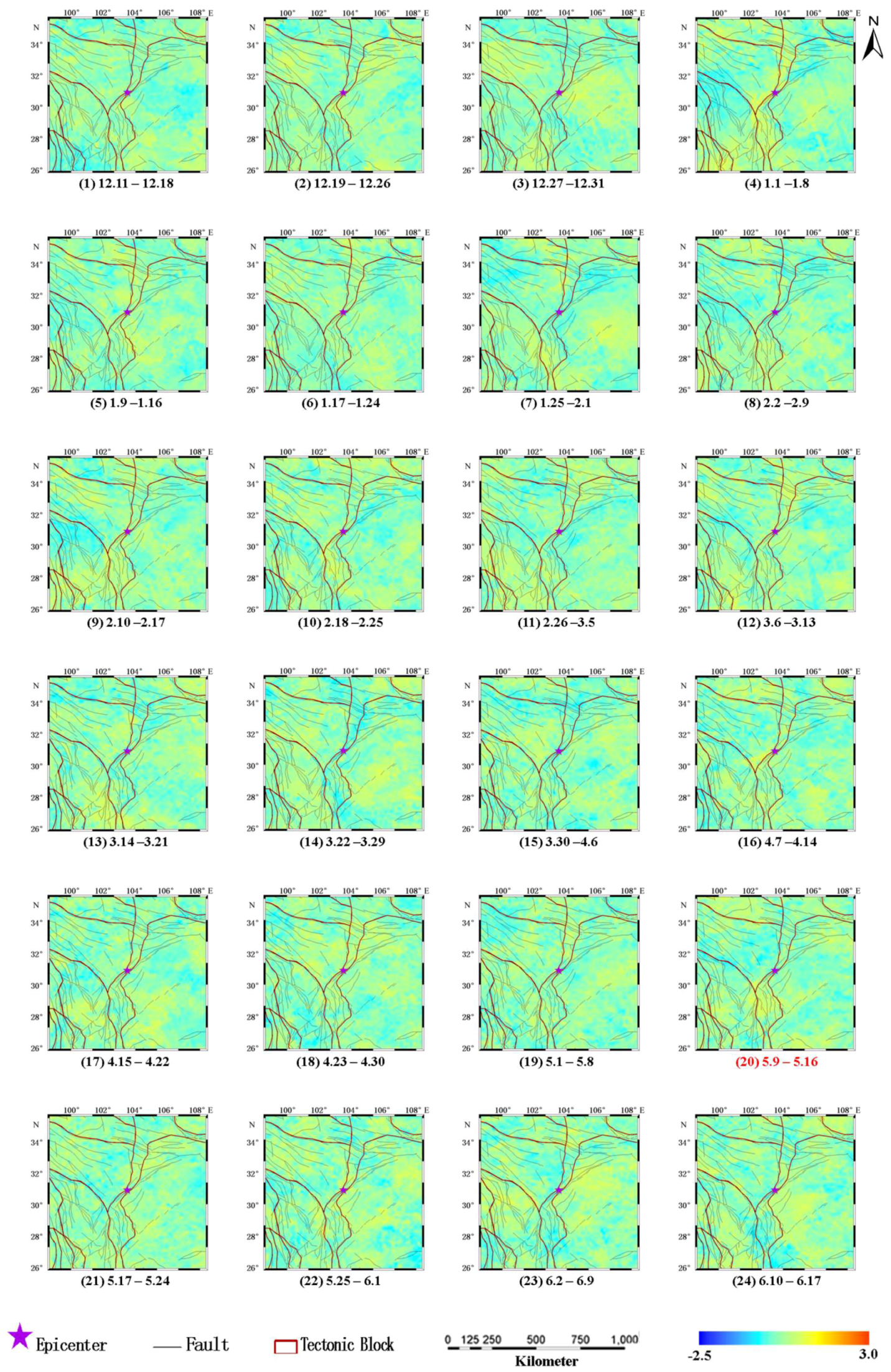
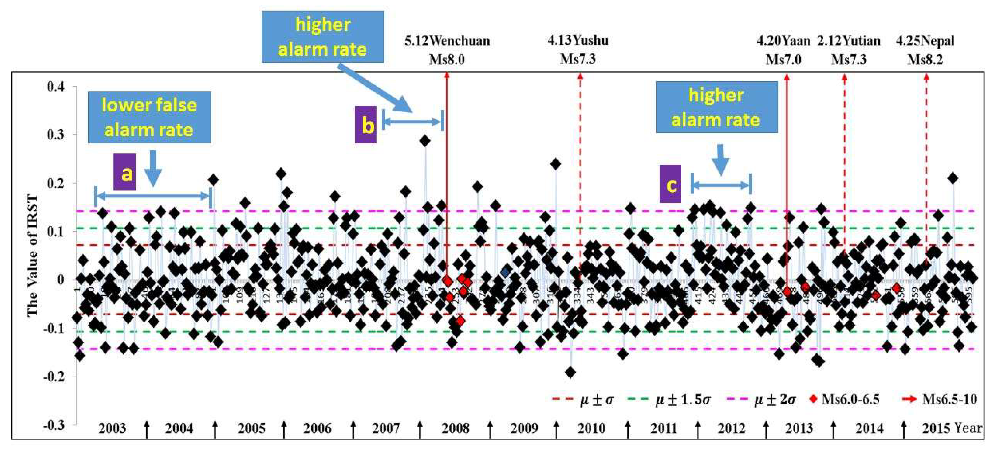
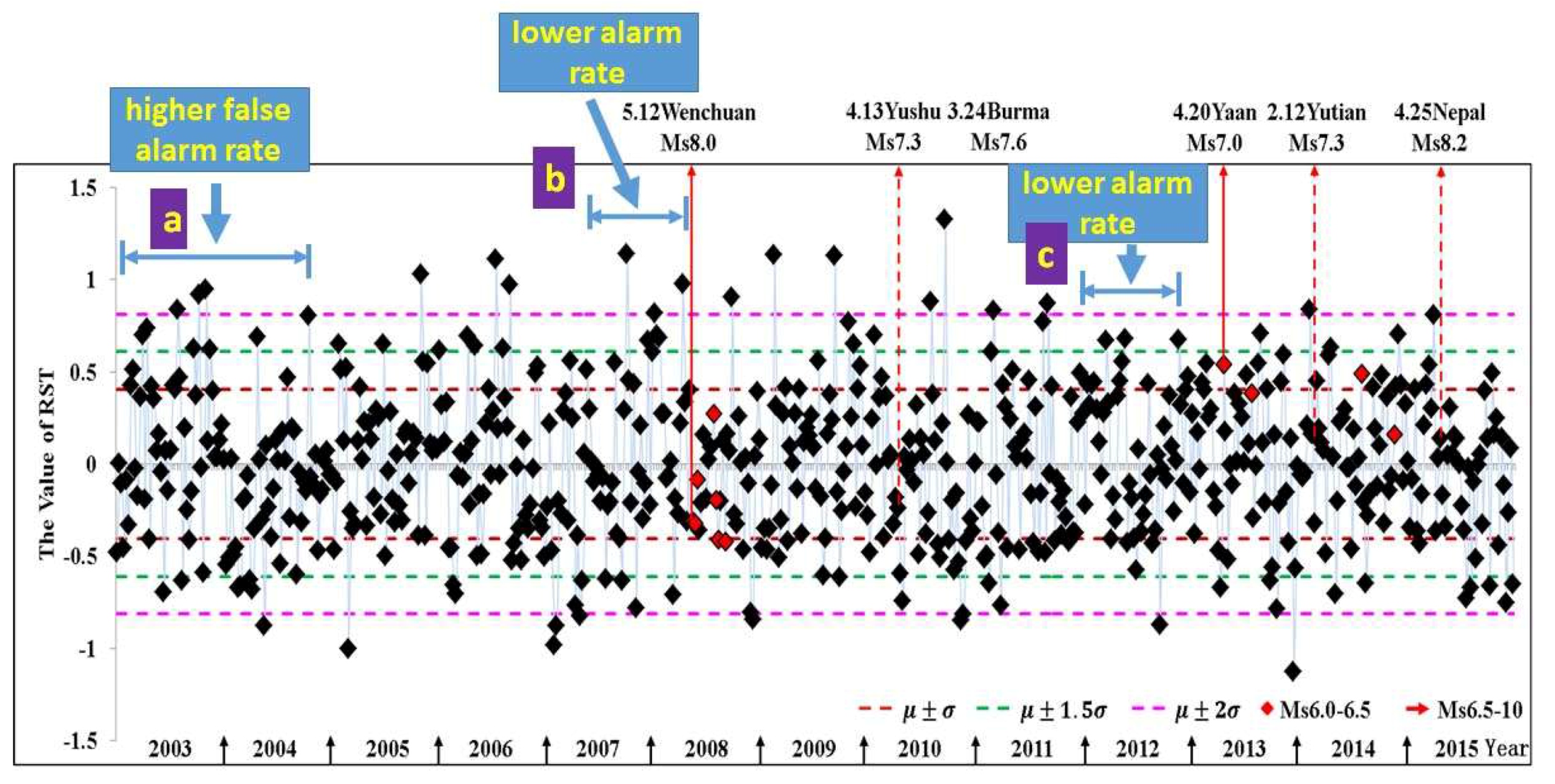
  • At the observe scale of earthquake generating fault zone, before the great earthquake, the fluctuations of the K t e c value are significantly more volatile than those in an aseismic period, which indicates that the TIR anomalies in tectonic activities in the event year are more active than those in non-event years.

Author Contributions

The following authors contributed to this study: D.S., R.X., J.Y., L.Z., X.S., and K.Q. conceived and designed the experiments; L.Z. and R.X. performed the experiments; K.Q., B.W. and J.C. contributed materials and analysis tools; and D.S. compiled and documented this study’s findings.

Funding

This research was funded by the National Science Foundation of China (41772350; 41401495; 61371189), and funded by the State Key Laboratory of Earthquake Dynamics (LED2012B02) and funded by the China Postdoctoral Science Foundation (2014M560463 and 2015T80603), and funded by the joint monitoring and analysis projections for the crust activities based on space imaging and earth surface observations were completed in Shanghai (14231202600; 16dz1206000). The authors would like to thank Shunyun Chen for his guidance during the process of performing this experimental study.

Conflicts of Interest

The authors declare no conflicts of interest.

References

  1. Freund, F. Pre-earthquake signals: Underlying physical processes. J. Asian Earth Sci. 2011, 41, 383–400. [Google Scholar] [CrossRef]
  2. Pulinets, S.A.; Dunajecka, M.A. Specific variations of air temperature and relative humidity around the time of Michoacan earthquake M8.1 Sept. 19, 1985 as a possible indicator of interaction between tectonic plates. Tectonophysics 2007, 431, 221–230. [Google Scholar] [CrossRef]
  3. Tronin, A.A.; Biagi, P.F.; Molchanov, O.A.; Khatkevich, Y.M.; Gordeev, E.I. Temperature variations related to earthquakes from simultaneous observation at the ground stations and by satellites in Kamchatka area. Phys. Chem. Earth 2004, 29, 501–506. [Google Scholar] [CrossRef]
  4. Roeloffs, E.A. Hydrologic precursors to earthquakes: A review. Pure Appl. Geophys. 1988, 126, 177–209. [Google Scholar] [CrossRef]
  5. Tronin, A.A. Remote sensing and earthquakes: A review. Phys. Chem. Earth Parts A/B/C 2006, 31, 138–142. [Google Scholar] [CrossRef] [Green Version]
  6. Qiang, Z.J.; Yao, Q.L.; Wei, L.J.; Zeng, Z.X. The characteristic of current stress hot field by satellite thermal infrared image in china. Acta Geosci. Sin. 2009, 30, 873–884. [Google Scholar]
  7. Choudhury, S.; Dasgupta, S.; Saraf, A.K.; Panda, S. Remote sensing observations of pre-earthquake thermal anomalies in Iran. Int. J. Remote Sens. 2006, 27, 4381–4396. [Google Scholar] [CrossRef]
  8. Ouzounov, D.; Bryant, N.; Logan, T.; Pulinets, S.; Taylor, P. Satellite thermal IR phenomena associated with some of the major earthquakes in 1999–2003. Phys. Chem. Earth Parts A/B/C 2006, 31, 154–163. [Google Scholar] [CrossRef]
  9. Saraf, A.K.; Rawat, V.; Banerjee, P.; Choudhury, S.; Panda, S.K.; Dasgupta, S.; Das, J.D. Satellite detection of earthquake thermal infrared precursors in Iran. Nat. Hazards 2008, 47, 119–135. [Google Scholar] [CrossRef]
  10. Saraf, A.K.; Rawat, V.; Das, J.; Zia, M.; Sharma, K. Satellite detection of thermal precursors of Yamnotri, Ravar and Dalbandin earthquakes. Nat. Hazards 2011, 61, 861–872. [Google Scholar] [CrossRef]
  11. Yao, Q.-L.; Qiang, Z.-J. Thermal infrared anomalies as a precursor of strong earthquakes in the distant future. Nat. Hazards 2012, 62, 991–1003. [Google Scholar] [CrossRef]
  12. Qiang, Z.J.; Xu, X.D.; Dian, C.G. Satellite thermal infrared anomalies—The pre-earthquake precursors. Chin. Sci. Bull. 1990, 35, 1324–1327. [Google Scholar]
  13. Piscini, A.; Santis, A.; Marchetti, D.; Cianchini, G. A Multi-parametric Climatological Approach to Study the 2016 Amatrice-Norcia (Central Italy) Earthquake Preparatory Phase. Pure Appl. Geophys. 2017, 174, 3673–3688. [Google Scholar] [CrossRef]
  14. Yadav, K.S.; Karia, S.P.; Pathak, K.N. Removal of solar radiation effect based on nonlinear data processing technique for seismo-ionospheric anomaly before few earthquakes. Geomat. Nat. Hazards Risk 2015, 7, 1147–1161. [Google Scholar] [CrossRef]
  15. Freund, F.; Keefner, J.; Mellon, J.J.; Post, R.; Takeuchi, A.; Lau, B.W.S.; La, A.; Ouzounov, D. Enhanced mid-infrared emission from igneous rocks under stress. Geophys. Res. Abstr. 2005, 7, 09568. [Google Scholar]
  16. Ishibashi, K. Two categories of earthquake precursors, physical and tectonic, and their roles in intermediate-term earthquake prediction. Pure Appl. Geophys. 1988, 126, 687–700. [Google Scholar] [CrossRef]
  17. Qiang, Z.J.; Xu, X.-D.; Dian, C.-G. Thermal infrared anomaly—Precursor of impending earthquakes. Chin. Sci. Bull. 1991, 36, 319–323. [Google Scholar] [CrossRef]
  18. Chen, S.Y.; Ma, J.; Liu, L.Q.; Liu, P. An enhancive phenomenon of thermal infrared radiation prior to Pakistan earthquake. Prog. Nat. Sci. 2006, 16, 1487–1490. [Google Scholar]
  19. Kai, Q. Preliminary analysis of surface temperature anomalies that preceded the two major Emilia 2012 earthquakes (Italy). Ann. Geophys. 2012, 55, 823–828. [Google Scholar]
  20. Bhardwaj, A.; Singh, S.; Sam, L.; Bhardwaj, A.; Martín-Torres, F.J.; Singh, A.; Kumar, R. MODIS-based estimates of strong snow surface temperature anomaly related to high altitude earthquakes of 2015. Remote Sens. Environ. 2017, 188, 1–8. [Google Scholar] [CrossRef]
  21. Genzano, N.; Aliano, C.; Corrado, R.; Filizzola, C.; Lisi, M.; Mazzeo, G.; Paciello, R.; Pergola, N.; Tramutoli, V. RST analysis of MSG-SEVIRI TIR radiances at the time of the Abruzzo 6 April 2009 earthquake. Nat. Hazard Earth Syst. Sci. Discuss. 2009, 9, 2073–2084. [Google Scholar] [CrossRef] [Green Version]
  22. Tramutoli, V. Robust Satellite Techniques (RST) for Natural and Environmental Hazards Monitoring and Mitigation: Theory and Applications. In Proceedings of the 2007 International Workshop on the Analysis of Multi-temporal Remote Sensing Images, Leuven, Belgium, 18–20 July 2007; pp. 1–6. [Google Scholar]
  23. Saraf, A.K.; Rawat, V.; Choudhury, S.; Dasgupta, S.; Das, J. Advances in understanding of the mechanism for generation of earthquake thermal precursors detected by satellites. Int. J. Appl. Earth Obs. Geoinf. 2009, 11, 373–379. [Google Scholar] [CrossRef]
  24. Tronin, A.A. Satellite thermal surveyâ a new tool for the study of seismoactive regions. Int. J. Remote Sens. 1996, 17, 1439–1455. [Google Scholar] [CrossRef]
  25. Tramutoli, V. Robust AVHRR techniques (RAT) for environmental monitoring: Theory and applications. Proc. SPIE 1998, 3496, 101–113. [Google Scholar]
  26. Tronin, A.A. Satellite thermal survey application for earthquake prediction. In Atmospheric and Ionospheric Electromagnetic Phenomena Associated with Earthquakes; Hayakawa, M., Ed.; Terrapub: Tokyo, Japan, 1999; pp. 717–746. [Google Scholar]
  27. Qiang, Z.J.; Dian, C.G.; Li, L.Z. Satellite thermal infrared precursors of two moderate-strong earthquakes in Japan and impending earthquake prediction. In Atmospheric and Ionospheric Electromagnetic Phenomena Associated with Earthquakes; Hayakawa, M., Ed.; Terrapub: Tokyo, Japan, 1999; pp. 747–750. [Google Scholar]
  28. Hayakawa, M.; Molchanov, O.A.; Kodama, T.; Tanaka, T.; Igarashi, T. On a possibility to monitor seismic activity using satellites. Adv. Space Res. 2000, 26, 993–996. [Google Scholar] [CrossRef]
  29. Tronin, A.A. Thermal IR satellite sensor data application for earthquake research in China. Int. J. Remote Sens. 2000, 21, 3169–3177. [Google Scholar] [CrossRef]
  30. Tronin, A.A. Thermal satellite data for earthquake research. In Proceedings of the IEEE 2000 International Geoscience and Remote Sensing Symposium, Honolulu, HI, USA, 24–28 July 2000; pp. 2703–2705. [Google Scholar]
  31. Tramutoli, V.; Bello, G.D.; Pergola, N.; Piscitelli, S. Robust satellite techniques for remote sensing of seismically active areas. Ann. Geophys. 2001, 44, 295–312. [Google Scholar]
  32. Tronin, A.A.; Hayakawa, M.; Molchanov, O.A. Thermal IR satellite data application for earthquake research in Japan and China. J. Geodyn. 2002, 33, 519–534. [Google Scholar] [CrossRef]
  33. Filizzola, C.; Pergola, N.; Pietrapertosa, C.; Tramutoli, V. Robust satellite techniques for seismically active areas monitoring: A sensitivity analysis on September 7, 1999 Athens’s earthquake. Phys. Chem. Earth 2004, 29, 517–527. [Google Scholar] [CrossRef]
  34. Ouzounov, D.; Freund, F. Mid-infrared emission prior to strong earthquakes analyzed by remote sensing data. Adv. Space Res. 2004, 33, 268–273. [Google Scholar] [CrossRef]
  35. Saraf, A.K.; Choudhury, S. Cover: NOAA-AVHRR detects thermal anomaly associated with the 26 January 2001 Bhuj earthquake, Gujarat, India. Int. J. Remote Sens. 2005, 26, 1065–1073. [Google Scholar] [CrossRef]
  36. Saraf, A.K.; Choudhury, S. Cover: Satellite detects surface thermal anomalies associated with the Algerian earthquakes of May 2003. Int. J. Remote Sens. 2005, 26, 2705–2713. [Google Scholar] [CrossRef]
  37. Saraf, A.K.; Choudhury, S. Thermal remote sensing technique in the study of pre-earthquake thermal anomalies. J. Ind. Geophys. Union 2005, 9, 197–207. [Google Scholar]
  38. Tramutoli, V.; Cuomo, V.; Filizzola, C.; Pergola, N.; Pietrapertosa, C. Assessing the potential of thermal infrared satellite surveys for monitoring seismically active areas: The case of Kocaell (Izmit) earthquake, August 17, 1999. Remote Sens. Environ. 2005, 96, 409–426. [Google Scholar] [CrossRef]
  39. Surkov, V.V.; Pokhotelov, O.A.; Parrot, M.; Hayakawa, M. On the origin of stable IR anomalies detected by satellites above seismo-active regions. Phys. Chem. Earth 2006, 31, 164–171. [Google Scholar] [CrossRef]
  40. Panda, S.K.; Choudhury, S. MODIS land surface temperature data detects thermal anomaly preceding 8 October 2005 Kashmir earthquake. Int. J. Remote Sens. 2007, 28, 4587–4596. [Google Scholar] [CrossRef]
  41. Rawat, V.; Saraf, A.K.; Sharma, K.; Shujat, Y. Anomalous land surface temperature and outgoing long-wave radiation observations prior to earthquakes in India and Romania. Nat. Hazards 2011, 59, 33–46. [Google Scholar] [CrossRef]
  42. Lisi, M.; Filizzola, C.; Genzano, N.; Paciello, R.; Pergola, N.; Tramutoli, V. Reducing atmospheric noise in RST analysis of TIR satellite radiances for earthquakes prone areas satellite monitoring. Phys. Chem. Earth Parts A/B/C 2015, 85–86, 87–97. [Google Scholar] [CrossRef]
  43. Ma, J.; Chen, S.; Hu, X.; Liu, P.; Liu, L. Spatial-temporal variation of the land surface temperature field and present-day tectonic activity. Geosci. Front. 2010, 1, 57–67. [Google Scholar] [CrossRef]
  44. Qiang, Z.J.; Kong, L.C.; Guo, M.H. The experimental study on the satellite thermal infrared heating mechanism. Acta Seismol. Sin. 1997, 19, 197–201. [Google Scholar]
  45. Wu, L.X.; Liu, S.J.; Wu, Y.H.; Li, Y.Q. Remote Sensing–Rock Mechanics (I)—Laws of thermal infrared radiation from fracturing of discontinuous jointed faults and its meanings for tectonic earthquake omens. Chin. J. Rock Mech. Eng. 2004, 23, 24–30. [Google Scholar]
  46. Wu, L.X.; Liu, S.J.; Wu, Y.H.; Li, Y.Q. Remote Sensing–Rock Mechanics (II)—Laws of thermal infrared radiation from viscosity-sliding of bi-sheared faults and its meanings for tectonic earthquake omens. Chin. J. Rock Mech. Eng. 2004, 23, 192–198. [Google Scholar]
  47. Wu, L.X.; Liu, S.J.; Wu, Y.H.; Li, Y.Q. Remote Sensing–Rock Mechanics (IV)—Laws of thermal infrared radiation from compressively-sheared fracturing of rock and its meanings for tectonic earthquake omens. Chin. J. Rock Mech. Eng. 2004, 23, 539–544. [Google Scholar]
  48. Piroddi, L.; Ranieri, G. Night Thermal Gradient: A New Potential Tool for Earthquake Precursors Studies. An Application to the Seismic Area of L’Aquila (Central Italy). IEEE J. STARS 2012, 5, 307–312. [Google Scholar] [CrossRef]
  49. Piroddi, L.; Ranieri, G.; Freund, F.; Trogu, A. Geology, tectonics and topography underlined by L’Aquila earthquake TIR precursors. Geophys. J. Int. 2014, 197, 1532–1536. [Google Scholar] [CrossRef]
  50. Ma, J.; Sherman, S.; Guo, Y.S. Recognition of stress state in the meta-instability stage before earthquake—Study on the evolution of temperature field in fault deformation with 5° bend. Sci. Chin. Earth Sci. 2012, 42, 633–645. [Google Scholar]
  51. Liu, P.; Ma, J.; Liu, L. An experimental study on variation of thermal fields during the deformation of a compressive en echelon fault set. Prog. Nat. Sci. 2007, 17, 298–304. [Google Scholar]
  52. Wu, L.; Liu, S.; Wu, Y. Precursors for rock fracturing and failure—Part II: IRR T-Curve abnormalities. Int. J. Rock Mech. Min. 2006, 43, 483–493. [Google Scholar] [CrossRef]
  53. Wu, L.; Liu, S.; Wu, Y. Precursors for rock fracturing and failure—Part I: IRR image abnormalities. Int. J. Rock Mech. Min. 2006, 43, 473–482. [Google Scholar] [CrossRef]
  54. Freund, F. Charge generation and propagation in igneous rocks. J. Geodyn. 2002, 33, 543–570. [Google Scholar] [CrossRef] [Green Version]
  55. Singh, R.P.; Kumar, J.S.; Zlotnicki, J.; Kafatos, M. Satellite detection of carbon monoxide emission prior to the Gujarat earthquake of 26 January 2001. Appl. Geochem. 2010, 25, 580–585. [Google Scholar] [CrossRef]
  56. Qiang, Z.; Dian, C.; Li, L.; Xu, M.; Ge, F.; Liu, T.; Zhao, Y.; Guo, M. Atellitic thermal infrared brightness temperature anomaly image—Short-term and impending earthquake precursors. Sci. China Ser. D 1999, 42, 313–324. [Google Scholar] [CrossRef]
  57. Qiang, Z.J.; Xu, X.D.; Dian, C.G. Case 27 thermal infrared anomaly precursor of impending earthquakes. Pure Appl. Geophys. 1991, 149, 319–323. [Google Scholar] [CrossRef]
  58. Chen, M.H.; Deng, Z.H.; MA, X.J.; Tao, J.L.; Wang, Y. Application of the inside-outside temperature relation analysis method in study on satellite infrared anomalies prior to earthquake. Seismol. Geol. 2007, 29, 863–872. [Google Scholar]
  59. Guo, W.Y.; Shan, X.J.; Ma, J. Discuss on the anomalous increase of ground temperature along the seismogenic fault before the Kunlunshan Ms8.1 earthquake in 2001. Seismol. Geol. 2004, 26, 548–556. [Google Scholar]
  60. Eleftheriou, A.; Filizzola, C.; Genzano, N.; Lacava, T.; Lisi, M.; Paciello, R.; Pergola, N.; Vallianatos, F.; Tramutoli, V. Long-term RST analysis of anomalous TIR sequences in relation with earthquakes occurred in Greece in the period 2004–2013. Pure Appl. Geophys. 2015, 173, 285–303. [Google Scholar] [CrossRef]
  61. Pergola, N.; Aliano, C.; Coviello, I.; Filizzola, C. Using RST approach and EOS-MODIS radiances for monitoring seismically active regions: A study on the 6 April 2009 Abruzzo earthquake. Nat. Hazards Earth Syst. Sci. 2010, 10, 239–249. [Google Scholar] [CrossRef]
  62. Blackett, M.; Wooster, M.J.; Malamud, B.D. Exploring land surface temperature earthquake precursors: A focus on the Gujarat (India) earthquake of 2001. Geophys. Res. Lett. 2011, 38. [Google Scholar] [CrossRef] [Green Version]
  63. Bellaoui, M.; Hassini, A.; Bouchouicha, K. Pre-seismic anomalies in remotely sensed land surface temperature measurements: The case study of 2003 Boumerdes earthquake. Adv. Space Res. 2017, 59, 2645–2657. [Google Scholar] [CrossRef]
  64. Chen, S.Y.; Liu, P.X.; Liu, L.Q.; Jin, M.A.; Chen, G.Q. Wavelet analysis of thermal infrared radiation of land surface and its implication in the study of current tectonic activities. Chin. J. Geophys. 2006, 49, 717–723. [Google Scholar] [CrossRef]
  65. Chen, S.Y. A Study on the Quantitative Thermal Infrared Remote Sensing Method for Extracting Information of Current Tectonic Activity. Ph.D. Thesis, Institute of Geology, China Earthquake Administration, Beijing, China, August 2006. [Google Scholar]
  66. Saradjian, M.R.; Akhoondzadeh, M. Thermal anomalies detection before strong earthquakes (M > 6.0) using interquartile, wavelet and kalman filter methods. Nat. Hazards Earth Syst. 2011, 11, 1099–1108. [Google Scholar] [CrossRef] [Green Version]
  67. Wang, Y.L.; Chen, G.H.; Kang, L.C.; Zhang, Q. Earthquake-related thermal infrared abnormity detection with wavelet packet decomposition. Prog. Geophys. 2008, 23, 368–374. [Google Scholar]
  68. Zhang, Y.S.; Guo, X.; Zhong, M.J.; Shen, W.R.; Li, W.; He, B. The satellite thermal infrared brightness temperature changes of Wenchuan earthquake. Chin. Sci. Bull. 2010, 55, 904–910. [Google Scholar]
  69. Zhang, X.; Zhang, Y.S.; Wei, C.X.; Tian, X.F.; Feng, H.W. Thermal infrared anomaly prior to Yiliang of Yunnan Ms5.7 earthquake. China Earthq. Eng. J. 2013, 35, 171–176. [Google Scholar]
  70. Chen, S.Y.; Jin, M.A.; Liu, P.X.; Liu, L.Q. A study on the normal annual variation field of land surface temperature in China. Chin. J. Geophys. 2009, 52, 2273–2281. [Google Scholar] [CrossRef]
  71. Li, Y.S. Numerical Approximation, Location of Publisher; People’s Education Press: Beijing, China, 1978. [Google Scholar]
  72. Li, D. Temporal-Spatial Structure of Intraplate Uplift in the Qinghai-Tibet Plateau. Acta Geol. Sin. (Engl. Ed.) 2010, 84, 105–134. [Google Scholar] [CrossRef]
  73. Cui, J.W.; Li, P.W.; Li, L. Uplift of the Qinhai-Tibet Plateau: Lithospheric structure and structural geomorphology of the Qinghai-Tibet Plateau. Cont. Dyn. 2001, 6, 29–37. [Google Scholar]
  74. Zhang, P.Z.; Deng, Q.D.; Zhan, G.M.; Ma, J. The activities of strong earthquakes and tectonic activities in China. Sci. China Ser. D 2003, 33, 12–20. [Google Scholar]
  75. Zhang, P.; Deng, Q.; Zhang, G.; Ma, J.; Gan, W.; Min, W.; Mao, F.; Wang, Q. Active tectonic blocks and strong earthquakes in the continent of China. Sci. Chin. 2003, 46, 13–24. [Google Scholar]
  76. Liu, X.; Ying, S.D.; Ma, J. Present-day deformation and stress state of Longmenshan fault from GPS results—Comparative research on active faults in Sichuan-Yunnan region. Chin. J. Geophys. 2014, 57, 1091–1100. [Google Scholar]
  77. Baiocchi, V.; Zottele, F.; Dominici, D. Remote sensing of urban microclimate change in L’Aquila city (Italy) after post-earthquake depopulation in an open source GIS environment. Sensors 2017, 17, 404. [Google Scholar] [CrossRef] [PubMed]
  78. Trigub, R.M.; Bellinsky, E.S. Fourier Analysis and Approximation of Functions; Kluwer Academic Publishers: Dordrech, The Netherlands, 2004. [Google Scholar]
  79. Zou, J.; Chen, J.; Geng, Z.M. Theory and application of optimal Fourier-Filter for waveform recovery. J. Vib. Eng. 2002, 15, 239–242. [Google Scholar]
  80. Liang, Z.G. Harmonic analysis of periodic signal. Meas. Technol. 2003, 2, 3–5. [Google Scholar]
  81. Lyon, M.; Picard, J. The Fourier approximation of smooth but non-periodic functions from unevenly spaced data. Adv. Comput. Math. 2014, 40, 1073–1092. [Google Scholar] [CrossRef]
  82. Zhang, X.; Zhang, R. The technology research in decomposition and reconstruction of image based on two-dimensional wavelet transform. In Proceedings of the IEEE International Conference on Fuzzy Systems and Knowledge Discovery, Changsha, China, 27–29 August 2000; pp. 1998–2000. [Google Scholar]
  83. Chen, S.Y.; Ma, W.; Liu, P.Y.; Liu, L.Q.; Yan, X.Y. Exploring the coseismic thermal response of Wenchuan earthquake using TERRA and AQUA satellite surface temperature. Chin. J. Geophys. 2013, 56, 3788–3799. [Google Scholar]
  84. Karl, T.R.; Diaz, H.F.; Kukla, G. Urbanization: Its detection and effect in the United States climate record. J. Clim. 1988, 1, 1099–1123. [Google Scholar] [CrossRef]
  85. Yuan, W.; Zou, L.Z.; Sun, J.Q. Temporal and Spatial Variation Characteristics of Summer Temperature in Xinjiang from 1951 to 2005 and Its Relationship with Atmospheric Circulation. J. Glaciol. Geocryol. 2009, 31, 801–807. [Google Scholar]
  86. Hou, W.; Sun, S.P.; Zhang, S.X.; Zhao, J.H.; Feng, G.L. Seasonal division of atmospheric circulation in East Asia and its temporal and spatial variation characteristics. Act Phys. Sin. 2011, 60, 781–789. [Google Scholar]
  87. Peng, S.L.; Zhou, K.; Ye, Y.H.; Su, J. Research progress in urban heat island effect. J. Ecol. Environ. 2005, 14, 574–579. [Google Scholar]
  88. Hu, Y.M.; Xu, C.G.; Bu, R.C.; Chang, W.; Zhang, Y.S. Application of Rs and Gis in Urban Heat Island Effect Research. Environ. Prot. Sci. 2002, 28, 1–3. [Google Scholar]
  89. Li, G.Q. Theories and Methods of Spatio-Temporal Outliers Detection. Ph.D. Thesis, Central South University, Changsha, China, 2009. [Google Scholar]
  90. Hawkins, D.M. Identification of Outliers; Chapman and Hall: London, UK, 1980; pp. 321–328. [Google Scholar]
  91. Jiang, S.Y.; Li, Q.H.; Li, K.L.; Wang, H. Glof: A new approach for mining local outlier. In Proceedings of the International Conference on Machine Learning and Cybernetics, Xi’an, China, 5 November 2003; Volume 151, pp. 157–162. [Google Scholar]
  92. Rousseeuw, P.J.; Leroy, A.M. Robust Regression and Outlier Detection; Wiley-Interscience: New York, NY, USA, 2003; pp. 260–261. [Google Scholar]
  93. Marchetti, D.; Akhoondzadeh, M. Analysis of Swarm satellites data showing seismoionospheric anomalies around the time of the strong Mexico (Mw =8.2) earthquake of 08 September 2017. Adv. Space Res. 2018, 62, 614–623. [Google Scholar] [CrossRef]
  94. Zhang, X.; Fidani, C.; Huang, J.; Shen, X. Burst increases of precipitating electrons recorded by the DEMETR satellite before strong earthquakes. Nat. Hazards Earth. Syst. 2013, 13, 197–209. [Google Scholar] [CrossRef]
Figure 1. Tectonic blocks and fault zones in the Qinghai-Tibet Plateau. The Yellow Border 1 on the left denotes the Altyn fault region; and the Yellow Border 2 on the right is the Longmenshan fault region. The sizes of these two sub-regions of the study area were both 10° × 10°.
Remotesensing 10 01941 g001
Figure 2. Distribution of the earthquake events in the Qinghai-Tibet Plateau from 2003 to 2015.
Remotesensing 10 01941 g002
Figure 3. Original images of the MODIS LST.
Remotesensing 10 01941 g003aRemotesensing 10 01941 g003b
Figure 4. Detailed flow chart of the proposed new algorithm.
Remotesensing 10 01941 g004
Figure 5. Detailed diagram of the proposed new algorithm.
Remotesensing 10 01941 g005
Figure 6. Sketch map of the “kσ” rule for detecting anomalies.
Remotesensing 10 01941 g006
Figure 7. Thermal infrared (TIR) anomalies spatio-temporal presentation of the Ms 8.0 Wenchuan earthquake based on the proposed tectonic thermal infrared anomalies (TTIA) method on the Tibetan Plateau.
Remotesensing 10 01941 g007
Figure 8. TIR anomalies prior to the Wenchuan earthquake event in different periods.
Remotesensing 10 01941 g008
Figure 9. Movement tendency of the TIR anomalies intensity centroid during the Wenchuan earthquake with (a) K t e c ≥ 1.0; and (b) K t e c ≥ 1.5.
Remotesensing 10 01941 g009
Figure 10. TIR anomalies spatio-temporal presentation of the Ms 7.3 Yutian earthquake based on the proposed TTIA method on the Tibetan Plateau.
Remotesensing 10 01941 g010aRemotesensing 10 01941 g010b
Figure 11. TIR anomalies prior to the Yutian earthquake event in different periods.
Remotesensing 10 01941 g011
Figure 12. Movement tendencies of the TIR anomalies intensity centroid during the Yutian earthquake event with: (a) K t e c ≥ 1.0; and (b) K t e c ≥ 1.5.
Remotesensing 10 01941 g012
Figure 13. Spatio-temporal evolution of K t e c extracted by the TTIA method in the Longmenshan fault region around the period Ms 8.0 Wenchuan earthquake breaking out in 2008. The date in red writing indicates the period that the earthquake happens.
Remotesensing 10 01941 g013
Figure 14. Spatio-temporal evolution of K t e c extracted by the TTIA method in the Longmenshan fault region in unperturbed period. The pixels values in images are the mean values of K t e c in the same time-slot of unperturbed periods.
Remotesensing 10 01941 g014
Figure 15. Spatio-temporal evolution of K t e c extracted by the TTIA method in the Altyn-Haiyuan fault region around the period of Ms 7.3 Yutian earthquake breaking out in 2014.
Remotesensing 10 01941 g015
Figure 16. Spatio-temporal evolution of K t e c based on the TTIA method in the Altyn-Haiyuan fault region in unperturbed periods. The pixel values in images are the mean values of K t e c in the same time-slot of unperturbed periods.
Remotesensing 10 01941 g016
Figure 17. Comparison of the temperature between from MODIS LST data and air temperature acquired by the Yutian meteorological ground station, and TIR anomaly based on the TTIA algorithm. The blue line denotes the daytime air temperature data observed by the ground site, the red line denotes the MODIS LST data at night, and the black line denotes the TIR anomaly based on the TTIA algorithm.
Remotesensing 10 01941 g017
Figure 18. TIR anomalies spatio-temporal presentation of the Ms 8.0 Wenchuan earthquake event based on the RST method on the Tibetan Plateau.
Remotesensing 10 01941 g018
Figure 19. Comparison of spatio-temporal evolution of TIR anomalies extracted by the RST method and TTIA method respectively in the Longmenshan fault region half a year to 2 months before the period Ms 8.0 Wenchuan earthquake event.
Remotesensing 10 01941 g019aRemotesensing 10 01941 g019b
Figure 20. Tectonic TIR anomalies in time series extracted by the TTIA method in the Longmenshan Fault zone.
Remotesensing 10 01941 g020
Figure 21. Tectonic TIR anomalies in time series extracted by the RST method in Longmenshan Fault.
Remotesensing 10 01941 g021
Figure 22. Presentation of the DEM, original MODIS LST data, and TIR anomalies bases on the TTIA method in Ms 8.0 Wenchuan earthquake event area.
Remotesensing 10 01941 g022
Figure 23. Presentation of the DEM, original MODIS LST data, and TIR anomalies based on the TTIA method and GPS displacement data on the Tibet-plateau area.
Remotesensing 10 01941 g023
Table 1. Data set of the MOD11A2.
NameData TypeEffective Numerical RangeUnitFilling ValuesCalibration Coefficient
LST_Day_1 km: 8-Day daytime
1 km grid LST
16-bit unsigned int7500–65535K00.02
QC_Day: Quality control for daytime LST and emissivity8-bit unsigned int0–255
Day_view_time: Average time of daytime LST observation8-bit unsigned int0–240h2550.1
Day_view_angle: Average view zenith angle of daytime LST 8-bit unsigned int0–130Degree2551(-65)
LST_Day_1 km:8-Day nighttime
1 km grid LST
16-bit unsigned int7500–65535K00.02
QC_Day: Quality control for nighttime LST and emissivity8-bit unsigned int0–255
Day_view_time: Average time of nighttime LST observation8-bit unsigned int0–240h2550.1
Day_view_angle: Average view zenith angle of nighttime LST8-bit unsigned int0–130Degree2551 (−65)
Emis_32: Band32 emissivity8-bit unsigned int1–255 00.002 (+0.49)
Emis_31: Band31 emissivity8-bit unsigned int1–255 00.002 (+0.49)
Clear_sky_days: the days in clear sky conditions and with valid LST8-bit unsigned int1–255 0
Clear_sky_nights: the nights in clear sky conditions and with valid LST8-bit unsigned int1–255 0

