Automated Attitude Determination for Pushbroom Sensors Based on Robust Image Matching
by
 , , , and
Ryu Sugimoto
1 ,
,
Toru Kouyama
1,*,
Atsunori Kanemura
1,
Soushi Kato
2,
Nevrez Imamoglu
1 and
Ryosuke Nakamura
1 1
National Institute of Advanced Industrial Science and Technology (AIST), Tokyo 135-0064, Japan
2
Remote Sensing Technology Center of Japan (RESTEC), Tokyo 105-0001, Japan
*
Author to whom correspondence should be addressed.
Remote Sens. 2018, 10(10), 1629; https://doi.org/10.3390/rs10101629
Submission received: 21 August 2018
/
Revised: 10 October 2018
/
Accepted: 11 October 2018
/
Published: 13 October 2018
(This article belongs to the Section Remote Sensing Image Processing)
Abstract
:Accurate attitude information from a satellite image sensor is essential for accurate map projection and reducing computational cost for post-processing of image registration, which enhance image usability, such as change detection. We propose a robust attitude-determination method for pushbroom sensors onboard spacecraft by matching land features in well registered base-map images and in observed images, which extends the current method that derives satellite attitude using an image taken with 2-D image sensors. Unlike 2-D image sensors, a pushbroom sensor observes the ground by changing its position and attitude according to the trajectory of a satellite. To address pushbroom-sensor observation, the proposed method can trace the temporal variation in the sensor attitude by combining the robust matching technique for a 2-D image sensor and a non-linear least squares approach, which can express gradual time evolution of the sensor attitude. Experimental results using images taken from a visible and near infrared pushbroom sensor of the Advanced Spaceborne Thermal Emission and Reflection Radiometer (ASTER) onboard Terra as test image and Landsat-8/OLI images as a base map show that the proposed method can determine satellite attitude with an accuracy of 0.003° (corresponding to the 2-pixel scale of ASTER) in roll and pitch angles even for a scene in which there are many cloud patches, whereas the determination accuracy remains 0.05° in the yaw angle that does not affect accuracy of image registration compared with the other two axes. In addition to the achieved attitude accuracy that was better than that using star trackers (0.01°) regarding roll and pitch angles, the proposed method does not require any attitude information from onboard sensors. Therefore, the proposed method may contribute to validating and calibrating attitude sensors in space, at the same time better accuracy will contribute to reducing computational cost in post-processing for image registration.
1. Introduction
Pushbroom-type image sensors have been widely used in Earth observation missions such as Landsat series, Terra, and Aqua. A pushbroom sensor is composed of 1-D detector(s) of which observations with a short interval according to satellite movement can provide 2-D observation images. Since 1-D instantaneous observation allows many pixels to be recorded in each image line compared to a 2-D image sensor, a pushbroom sensor can provide high-spatial-resolution images with a wide enough swath length. Based on this advantage, for example, visible and near infrared images with a high spatial resolution have been used for monitoring temporal variation in land use, and thermal infrared images have been used for determining exact locations of active volcanoes that have high-temperature anomalies. For these analyses, accurate geo-location of a target is essential; thus, accurate map projection of an observed image is necessary.
Although several methods have been proposed to determine the precise location of a observed scene by matching an observed image to a reference image (or base-map image) whose geo-location is accurately determined, these methods start with a map product of an observed image which is already projected based on satellite position and attitude measured using sensors onboard a satellite cf. [1,2]. Because a sensor onboard a satellite captures a target from space, a small error in attitude inevitably causes a large position error of a target on the surface (e.g., 1° error for a 700-km-altitude satellite causes a 10-km displacement on the surface), which leads to the necessity of a large search range for matching observed and reference images; thus, huge computational cost is needed for the matching. Therefore, accurate satellite or sensor attitude determination is important for providing a sufficiently accurate map product, of which precise image matching can be conducted in a postprocessing stage with low computational cost. Common available methods for attitude determinations are using star trackers (STTs), sun sensors, gyroscopes, geomagnetic sensors, and horizon sensors [3]. STTs can provide much more accurate absolute attitude information (the order of 0.01°) than the others.
Japan has a future hyperspectral mission, called Hyper-spectral Imager SUIte (HISUI), which will be installed on the Japanese Experiment Module (JEM) of the International Space Station (ISS) in 2019 [4]. HISUI is a pushbroom type hyperspectral imager whose spectral coverage is 0.4–2.5 μm with intervals of 10 nm in visible and near infrared wavelength ranges and 12.5 nm in shortwave infrared wavelength range, respectively [4,5]. Planned spatial resolution of the HISUI is 30 m. Similar to other satellite missions, the HISUI mission plans to provide map-projected image products. Unlike a satellite, the ISS is a huge platform composed of many modules and living spaces, and there are many vibration modes that may affect sensor attitudes during observations cf. [6]. Therefore, a sensor on the JEM usually has its own attitude sensors such as STTs and/or attitude determination schemes cf. [7] to accurately determine sensor attitude at each observation. HISUI will include an STT for determining its attitude during image acquisition [4]. On the JEM, however, it is expected that attitude determination by STTs will be somewhat limited because half of an STT’s field of view will be covered by large solar panels and large modules of the ISS [8], which will reduce the number of stars in an STT’s field of view. In addition, considering contamination of sunlight and reflected sunlight by solar panels and modules in an STT’s field of view, attitude information from STTs may not be available for a while.
To address this problem, we propose an attitude-determination method for pushbroom sensors that is only based on observed images with known satellite positions. Thus, it does not require any attitude information from onboard sensors. This method is an expansion of an attitude-determination method for 2-D frame sensors proposed in [9], which uses an observed scene for determining sensor attitude, and achieves better accuracy of attitude-determination than that of STTs and at the same time is robust against occurrences of clouds in the scene. Several methods have been proposed and evaluated for attitude determination by taking advantage of reference Ground Control Points (GCPs) extracted from pushbroom images [10,11,12,13,14,15]. Attitude determination from these studies using GCPs as reference resulted in better accuracy than that of onboard attitude sensors, while they examined their methods with manually extracted GCPs cf. [13], GCPs with specified locations [15], or GCPs automatically extracted by an image processing technique but starting from already map projected images based on onboard sensors [11]. Moreover, robustness of these methods, especially on the scenes with clouds, has not been discussed since GCP locations were obtained by the clear weather scenes. Therefore, in this work, we introduce a robust attitude determination method that uses only observed images that can handle various scene conditions (e.g., scenes with many clouds) without any prior attitude information.
The novelty of this study is that we successfully retrieve temporal variation of sensor attitude robustly even for a scene with many clouds. We achieve this by combining (1) a robust and automated GCP selection, (2) a rough sensor attitude determination method, and (3) solving temporal variation of sensor attitude with a non-linear least square approach.
As in [9], the fundamental idea of the proposed method is the automated matching of pairs of feature points, where one set of points is extracted from a base map with known latitude and longitude and the other is extracted from a satellite image with unknown attitude parameters. Borrowing ideas from computer vision, the method combines feature-point detection with speeded up robust features (SURF) [16], a robust estimation algorithm (i.e., the random sample consensus (RANSAC) family [17,18]) for determining rough attitude parameters, and a non-linear least squares approach for deriving precise sensor attitude, which changes with time.
In Section 2, we describe the mathematical basis of our method based on satellite observation geometry with a pushbroom sensor using land-feature matching and outlier rejection by robust estimation. In Section 3, we introduce the satellite imagery datasets used for testing and explain the experimental results of the proposed method. In Section 4, we discuss the performance of our proposed method and suggest ways to determine sensor attitude when less feature points are available. Section 5 concludes the paper.
2. Method
2.1. Overview of Proposed Method
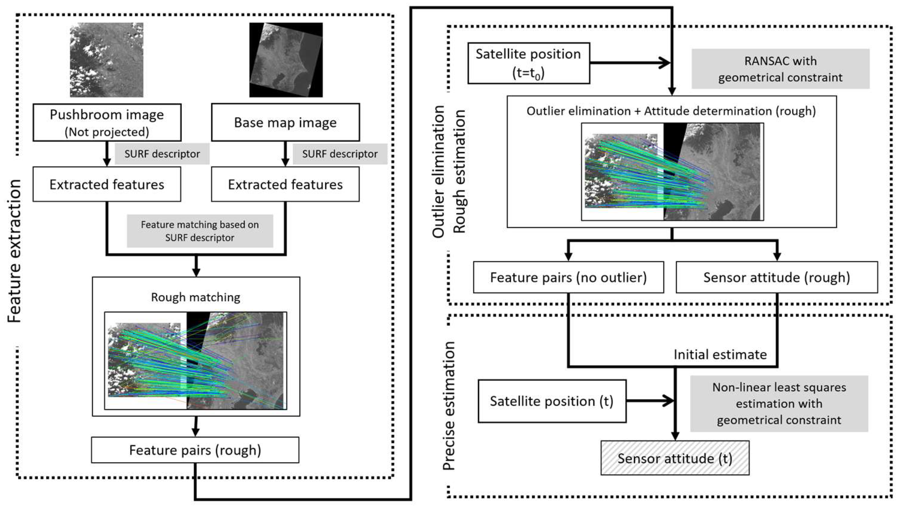
The proposed method consists of three major steps: (1) matching feature pairs between an observed image (before projection) and base-map image based on only feature similarities, (2) eliminating incorrectly matched pairs by robust image processing with a geometric constraint between the extracted feature points and satellite position and at the same time estimating sensor attitude roughly assuming a pushbroom image is taken from a certain satellite position, and (3) precisely deriving sensor attitude including its temporal variation based on the geometric constraint at each scan line. Figure 1 shows a flowchart of the proposed scheme.
As with [9], the first step consists of the following sub-steps: (1-1) extracting feature points from a base map with known latitude and longitude and from a satellite image with unknown attitude parameters using SURF; and (1-2) matching pairs of these feature points roughly based on SURF descriptors. The second step consists of the following sub-steps: (2-1) eliminating incorrect feature pairs, or outliers, with RANSAC or its variant using the geometric constraints; and (2-2) deriving satellite attitude from remaining inliers. The approach in (2) is based on Kouyama et al.’s robust scheme [9]. Since the attitude determination method in [9] assumes a 2-D image frame sensor, we assume in step (2) that a pushbroom image is taken at a certain position and attitude, such as a 2-D frame sensor image.
In following subsections, we first provide the mathematical basis of satellite attitude determination from an observed image with known satellite position, discuss how we extract and match feature pairs from satellite and base-map images, then how we determine sensor attitude including its temporal variation.
2.2. Mathematical Basis of Attitude Determination for a Pushbroom Sensor
The previous attitude-determination method in [9] used the geometrical fact that we can uniquely determine the Earth’s appearance seen from a satellite position when the trajectory (latitude, longitude, and altitude) of a satellite and its attitude are given. Conversely, we can then determine satellite attitude uniquely by matching the Earth’s appearance in a satellite image (not projected) to the expected Earth’s appearance from the satellite. However, there is a strict assumption that the entire observed region in an image are captured at the same time.
When a pushbroom sensor scans the Earth’s surface, both its position and attitude change during one observation sequence. To determine attitude of a pushbroom sensor, the temporal variation in sensor position and attitude must be taken into account, which is not necessary with 2-D image sensors. In this section, we formulate the geometrical relationship between the feature points extracted from a pushbroom image and their corresponding positions on the Earth whose latitude, longitude, and altitude are given. We adopted a bundle-adjustment approach for deriving the temporal variation in sensor attitude by solving a non-linear least squares problem, which has been established in photogrammetry and widely used in photogrammetric and many other research fields cf. [12,19], and see Appendix A including remote sensing studies, such as on deriving sensor attitude onboard air planes [11].
We first define a feature-pointing vector representing the direction of each extracted land feature in a pushbroom image. For the i-th land feature in the image, we specify a unit vector pointing from the satellite position to a land position , where represents the observation time when the land position is captured by the sensor. The planetographic longitude, latitude, and altitude of Pi, denoted as , , and , respectively, are described in Earth-centered coordinates (Figure 2a) as
where is the equatorial radius of Earth, is the pole radius, and is radius of curvature in prime vertical defined in terms of , , and the eccentricity of Earth (),
We adopted and the value of inverse flattening based on World Geodetic System 1984 (WGS 84). We assumed that a satellite position in (1) is given; thus, is treated as a known variable.
Next, we represent the same vector in the camera-centered coordinate system, with origin at the pinhole position of the camera onboard the satellite (Figure 2b). In this coordinate system, is represented by a vector , which is expressed in terms of the projected position of on the detector plane, , as
where is the focal length of the sensor.
As with 2-D image sensors, and point in the same direction but are expressed in different coordinate systems. Using a rotation matrix, , that connects the Earth-centered coordinate to the camera-centered coordinate systems,
we can describe the relationship between and directly through as follows:
We modified (5) based on (3) as follows:
This equation is equivalent to the collinearity equation that satisfies a geometrical constraint that a target point on the Earth’s surface, the origin of camera coordinate (S in Figure 2b), and a projected point on the detector plane are in a line. Supposing that we have n-matched pairs, we have n sets of the equations in (6).
It should be emphasized that because both the position and attitude of a pushbroom sensor vary at every scan line (i.e., varies with time), a method of attitude determination of a pushbroom sensor should be able to treat the temporal variation of . This is a fundamental difference from attitude determination with 2-D image sensors. During usual observation, a satellite changes its attitude gradually (not discretely) to keep a boresight vector of a sensor directed to the Earth’s surface following the satellite motion. To treat this gradual temporal variation in sensor attitude, we express with roll (), pitch () and yaw () angles as
with temporal variation terms
where , , and represent such angles at , respectively, and , , and correspond to angular velocities of the angles with a unit of radian per second. The sensor attitude is expressed in Earth-centered coordinates with Euler angles, and the rotation order of Euler rotation is roll, pitch, and yaw (X-Y-Z).
Finding is equivalent to finding the six parameters of , , and this problem can be considered as a parameter search with a non-linear least squares method, which minimizes
The linear expressions of sensor attitude variation in (8) are valid only for a sensor with constant rotation. Even though sensors generally have some drift from the constant rotation rate, our experimental results have shown that the linear equations can provide enough accuracy for ASTER case (see Section 3.3). We also examined the derivation of sensor attitude with a combination of linear and quadratic equations (see Section 4.2) for obtaining more accurate attitude information when the drift of a pushbroom sensor is not negligible.
Once we have M(t), then we can calculate a line-of-sight direction from a pixel to the Earth’s surface with the given satellite position and obtain the corresponding longitude, latitude, and elevation of the pixel by calculating a location where the line-of-sight vector and Earth’s surface intersect. Above, we assumed that the satellite position is accurately determined for each scan line.
2.3. Robust Estimation of Initial Estimates and Elimination of Incorreclly Matched Feature Pairs
A non-linear least squares method requires the provision of initial estimates of the six parameters of , , which should be close to the actual values. We first set based on an assumption of small variation of sensor attitude in a single scene. Then, to obtain the initial estimates of , we followed Kouyama et al.’s scheme [9], which can robustly derive sensor attitude and at the same time exclude incorrectly matched feature pairs by using only the observed and base map images. We did not use any attitude information from onboard sensors for the initial estimates to address a situation that any onboard attitude sensor cannot determine attitude of a pushbroom sensor enough accurately. This situation may occur for a sensor onboard JEM on the ISS, as described in the introduction section.
Firstly, since the scheme proposed in [9] is for a 2-D frame sensor, we assumed that the pushbroom image is taken by a 2-D frame sensor at , which corresponds to be the scene center time, for adapting the scheme for a pushbroom observation. Then, we identified feature points in the observed and base map images by using the SURF feature descriptor. We used the 128-dimensional descriptor due to providing more distinctive information as stated in [20]. SURF has been implemented by an open source framework, OpenCV [21]. Since SURF descriptors take similar values if feature points are similar to each other, they can be used to discover corresponding points in different images by measuring the Euclidean distances between the extracted features. However, the result may include incorrectly matched pairs because of the existence of similar features in the scenes and well-known problem of distance metrics including Euclidean distance on high-dimensional space.
Next, we adopted a robust statistical approach proposed in [9] which uses RANSAC, or progressive SAC (PROSAC) [22], with a geometrical constraint of satellite observation to eliminate the incorrectly matched pairs. The statistical approach for eliminating incorrectly matched pairs utilizes the characteristic that incorrectly matched feature points have no geometrical relationships to each other, and thus they should reveal much larger geometrical inconsistencies than that of the correctly matched pairs. This step is required because the mathematical basis discussed in the previous sub-section assumes that all feature pairs are correctly matched ones. For instance, as reported in [9], an incorrectly matched pair may cause large attitude errors which could lead to 10 degrees attitude errors (corresponding to 100 km error). Therefore, it is crucial that all incorrectly matched pairs should be eliminated.
The geometrical inconsistency of a feature pair can be measured from a comparison of the two vector directions, and , which are expected to be same as follows,
In this study, we adopted 0.2° as a threshold for distinguishing between correctly and incorrectly matched feature pairs following [9]. Through the process of RANSAC we can exclude all incorrectly matched pairs and at the same time obtain correct sensor attitude, which can be converted to the initial estimate of and .
Advantages of applying the robust attitude determination scheme for a 2-D frame sensor in [9] are: (1) it can robustly provide correct matched pairs and initial estimates of and without any manual process, and (2) thanks to the robustness on feature matching and initial estimate of parameters, it can provide sensor attitude even for the partially or highly cloudy scenes.
3. Results
This section describes the satellite images used for attitude determination and the images used as the base map, results of sensor attitude determination based on the proposed method, and error evaluation of the determination.
3.1. Test Data Sets
3.1.1. ASTER Images: Raw Pushbroom Images
ASTER is a mid-resolution pushbroom sensor onboard Terra, which was launched in 1999. Terra has orbited at 704-km altitude and ASTER has observed the Earth’s surface successfully and continuously since the launch. The ASTER project has provided both non-projected images (so called Level 1A products) and images projected onto a map coordinate via the LP DAAC web service [23]. In these products, satellite information is also included, which can be used for evaluating the position and attitude of ASTER at each scan line. Additionally, the ASTER project has provided sight vectors in L1A products which are equivalent to line-of-sight vector directions for each pixel in ASTER’s camera-centered coordinate, and using the direction, we can obtain accurate . Note that ASTER does not have any clear optical distortion and the direction of the line-of-sight vector for each pixel of ASTER is well determined in ASTER’s camera coordinate [24], and Terra’s position during an observation is determined by the Tracking Data Relay Satellite On-Board Navigation System (TONS) [25] with an accuracy better than 100 m [26]. Given these characteristics, the ASTER images are suitable for this study as a raw pushbroom images which are not projected onto a map coordinate. In this study, we used Band 1 images, and the specifications of ASTER Band 1 are summarized in Table 1.
3.1.2. Landsat-8/OLI Images: Base-Map Images
Landsat-8’s Operational Land Imager (OLI) is a mid-resolution satellite optical sensor launched in 2013. As published OLI images have already been projected onto a map coordinate, the latitude and longitude of each pixel in the images can be determined from the map-projection information distributed by the United States Geological Survey (USGS). The reported accuracy of the map projection is 18 m [27]. We used Band 3 images as the base map images, whose wavelength is included in the ASTER Band 1 coverage. The specifications of OLI (Band 3) are summarized in Table 2.
Since Landsat-8 has observed almost all over the world, its dataset is an ideal one for our purpose. We found the 18-m accuracy is enough for our method to provide sensor attitude with a comparable accuracy to STTs (see Section 3).
The elevation of each pixel can be determined using a digital elevation model (DEM). We used a DEM generated from ASTER data with a ground sampling distance (GSD) of 30 m [28,29]. Although ASTER also has its own map product, it is more realistic to use an already existing map product as a base map from another satellite mission when we apply our proposed method for determining sensor attitude.
3.2. Sensor Attitude Determination
3.2.1. Robust Determination of Sensor Attitude (Rough) and Extracting Correctly Matched Feature Pairs
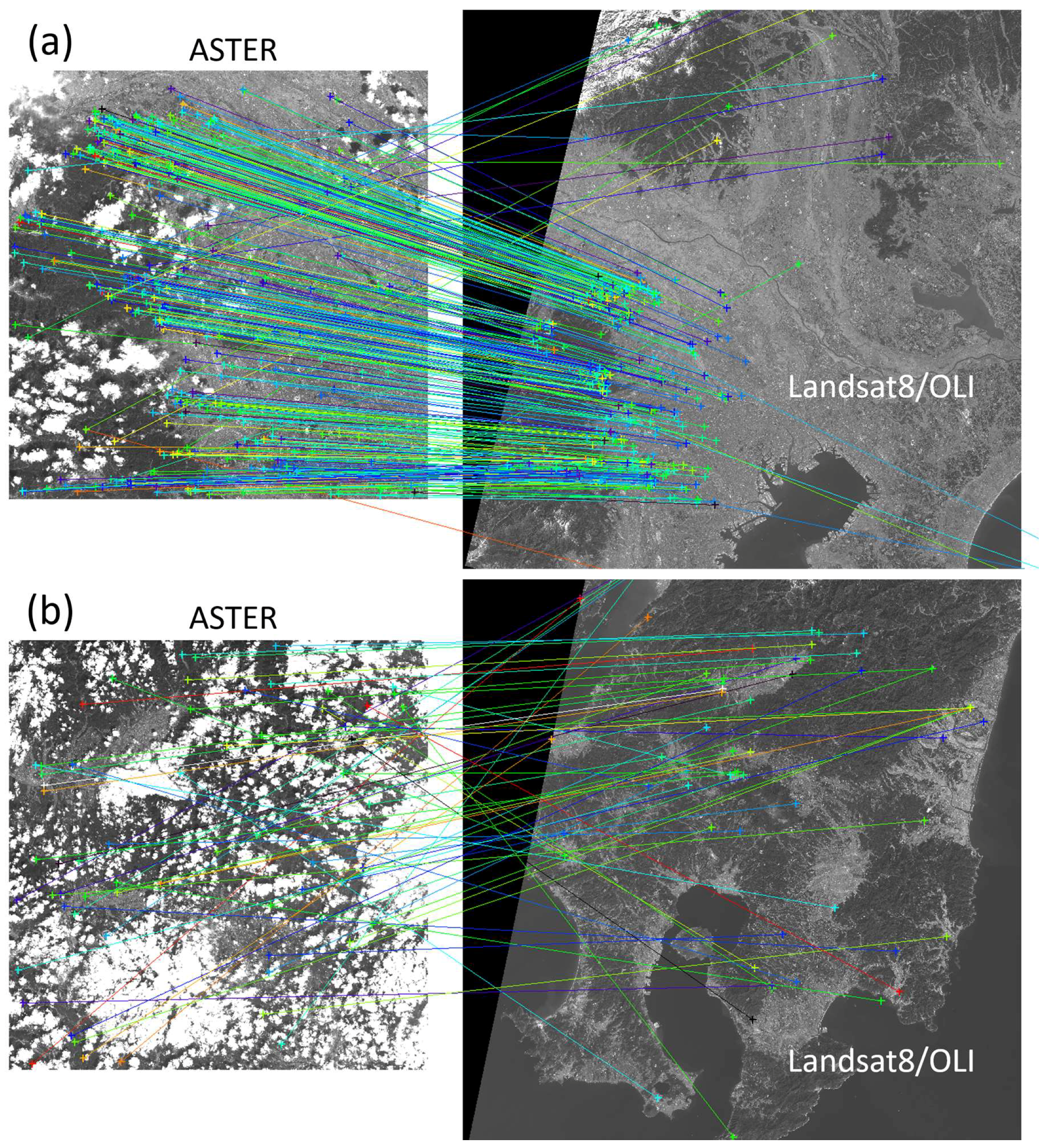
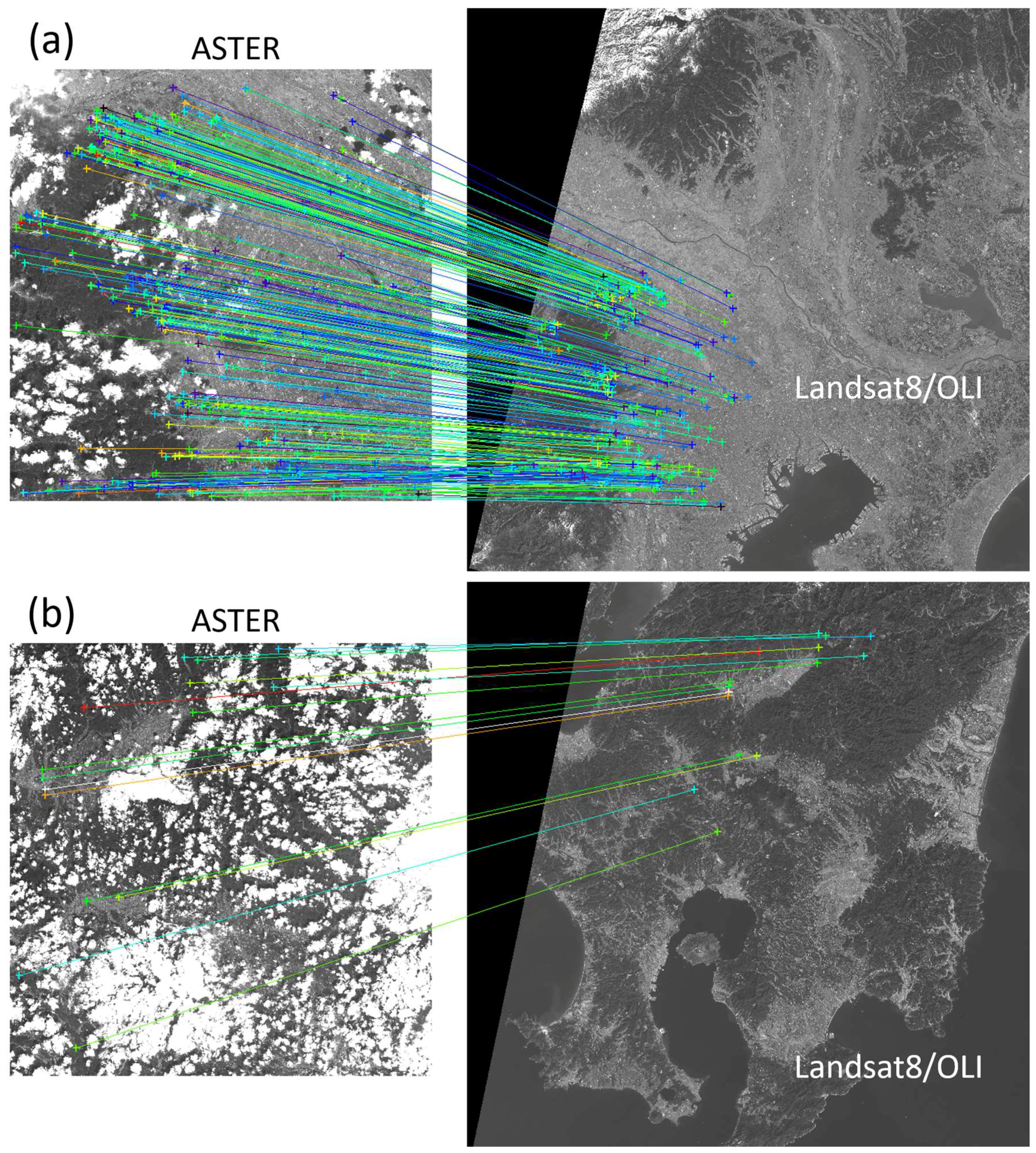
Figure 3 presents examples of feature matching between raw and mapped images only based on the SURF descriptors (rough matching), and Figure 4 presents feature-matching results with an additional algorithm (correct matching). The observed images in Figure 3a and Figure 4a show the Kanto area (Japan) in which clouds covered few parts of the scene, and the observed images in Figure 3b and Figure 4b show the Kyushu areas (Japan) in which clouds covered many parts of the scene. In the Kyushu case, though there were many obvious incorrectly matched pairs in the rough matching phase due to many cloud patches (Figure 3b), obvious failed pairs were completely excluded in the correct matching phase (Figure 4b). The numbers of the remaining correctly matched pairs were 389 and 16 for Kanto and Kyushu cases, respectively. We confirmed that all remaining feature pairs in Figure 4 showed good consistency between and , which are better than 0.012°, thus they can be considered correctly matched pairs.
3.2.2. Precise Determination of Sensor Attitude and Its Accuracy
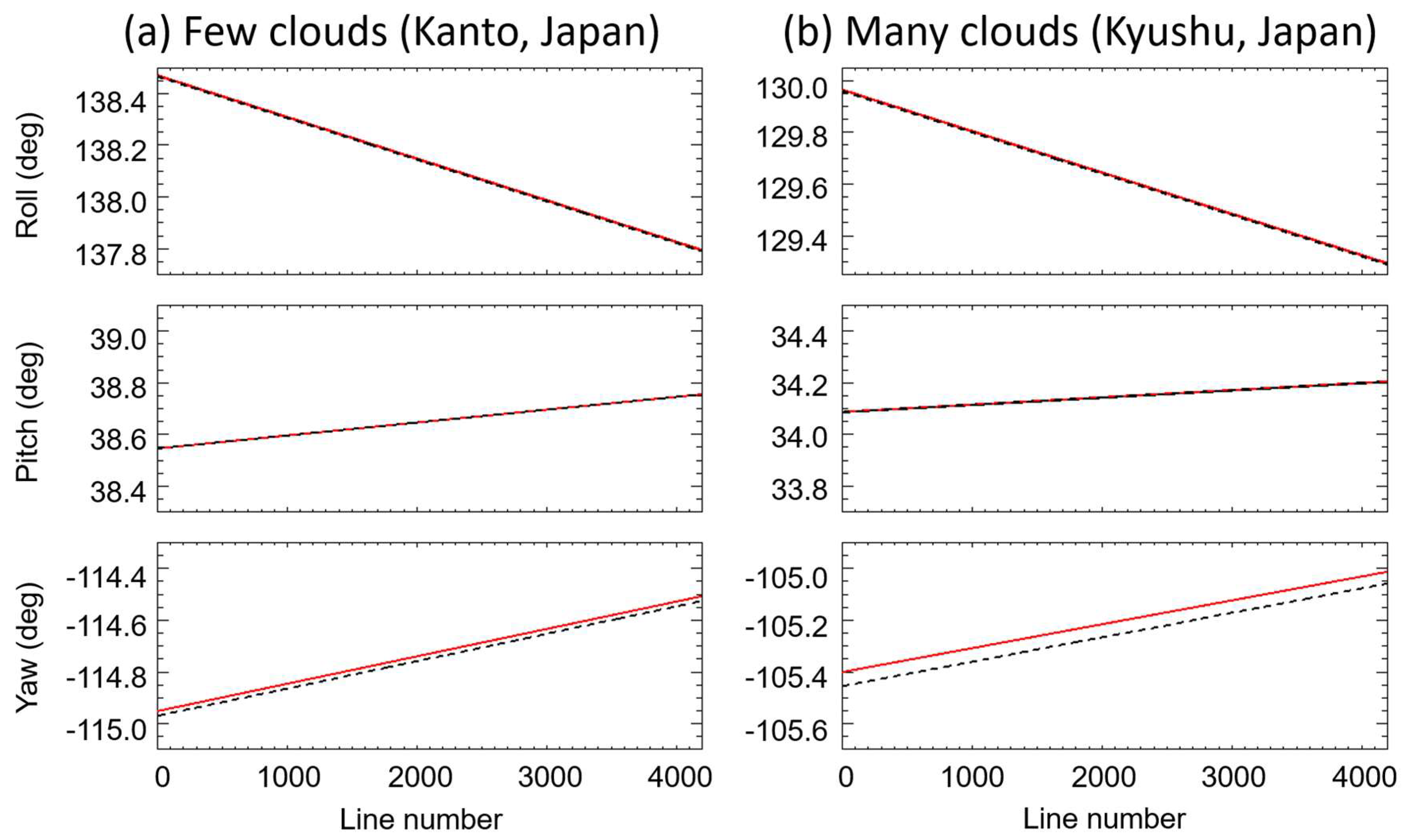
In the previous section, we obtained a rough estimation of sensor attitude based on a 2-D frame sensor assumption and correctly matched feature pairs between pushbroom and base-map images. Using the correctly matched pairs and the estimated sensor attitude parameters as initial values of , , and in (8), we successfully obtained temporal variation in sensor attitude expressed with roll, pitch, and yaw angles as functions of time (Figure 5) by solving a non-linear least squares problem of (9). Comparing attitude information provided in the ASTER Level 1A products, which was determined from an STT given every ~400 pixels (corresponding to ~1 Hz sampling), sensor attitude based on the precise procedure suggested the same variation trends for scenes with both few and many clouds, while a systematic 0.05° difference was observed in the yaw angle for scenes with many clouds.
3.3. Acuracy of Determined Sensor Attitude
3.3.1. Map-Projection Accuracy
To validate the accuracy of the sensor attitude obtained from the precise procedure, we again carried out map projection of ASTER images with the attitude measured in the previous subsection and the given satellite positions. Figure 6 shows examples of the map projection of ASTER images in which features were smoothly connected across image boundaries.
The absolute accuracy of sensor attitude was assessed based on the registration errors of the map projection, defined as the differences between the detected feature points in map-projected ASTER and base-map images, that is, the latitude–longitude displacement between matched features extracted from the OLI base-map and projected ASTER images with the proposed method. As in [9], since the ASTER and OLI images have different GSDs, SURF descriptor was used again to find the corresponding points from a pair of ASTER and OLI images using SURF’s characteristics of scale invariance and sub-pixel level accuracy. The mean displacements of feature points, which indicate the absolute geometric accuracy of registration, and the root mean square errors (RMSEs) for indicating relative miss-registration errors were calculated in the east–west and north–south directions of the two images in Figure 6 (Table 3). Regardless of the amount of clouds in a scene, mean discrepancy in both east–west and north–south directions were smaller than 6 m, and RMSEs in both west-east and north-south directions were smaller than 15 m in both cases from the proposed method. These values are better than those from the map projection based on onboard sensors (Table 3). Total RMSEs were smaller than 27 m, which includes the reported registration error in the Landsat-8/OLI map product (18 m) and the measured RMSEs in west-east and north-south directions. The RMSE of 27 m corresponds to the two-pixel spatial scale of an ASTER image. Considering that reported accuracies of sensor attitude determination based on observed images were also one or two-pixel spatial scale of a sensor, as found in previous studies [9,11], the accuracy of attitude determination based on satellite images may depend on the spatial resolution of a sensor. It is worth investigating this dependence in future work.
Since ASTER observed the Earth’s surface from 704 km altitude, the accuracy of the proposed method corresponds to ~0.003° in roll and pitch angles and ~0.05° in yaw angle. The reason of the large error range in yaw angle comes from the fact that and are less sensitive to the rotation around the yaw axis than rotations around the roll and pitch axes. Rotations around the roll and pitch axes linearly affect the discrepancies in the x and y directions, respectively, which are proportional to the sensor altitude (i.e., , where is sensor altitude). On the other hand, since we set the order of rotation M as roll, pitch and yaw in this study, the direction of the yaw axis is same as the direction of boresight vector of ASTER. Therefore, the rotation around the yaw axis corresponds to rotating an image frame, and the discrepancy is proportional to , where represents the distance between a boresight point on the Earth’s surface and a point where a line-of-sight vector intersects with the Earth surface in each scan line (i.e., ). takes its maximum at the edge of the sensor swath. In the ASTER case whose swath width is 60 km (much shorter than the sensor altitude, 704 km), the error range of 27 m corresponds to 0.05° yaw rotation at the edge of its swath. Though large uncertainty remains in the yaw angle, the proposed method can precisely determine roll and pitch angle rotations, which should be better than 0.01° from analyses of miss-registration errors in the ASTER case.
3.3.2. Comparison with Sensor Attitude from Onboard Sensors
The difference between sensor attitudes measured from the Terra/ASTER onboard sensors and the proposed method can be evaluated from a matrix, , that represents the difference between two attitudes at each time step as follows:
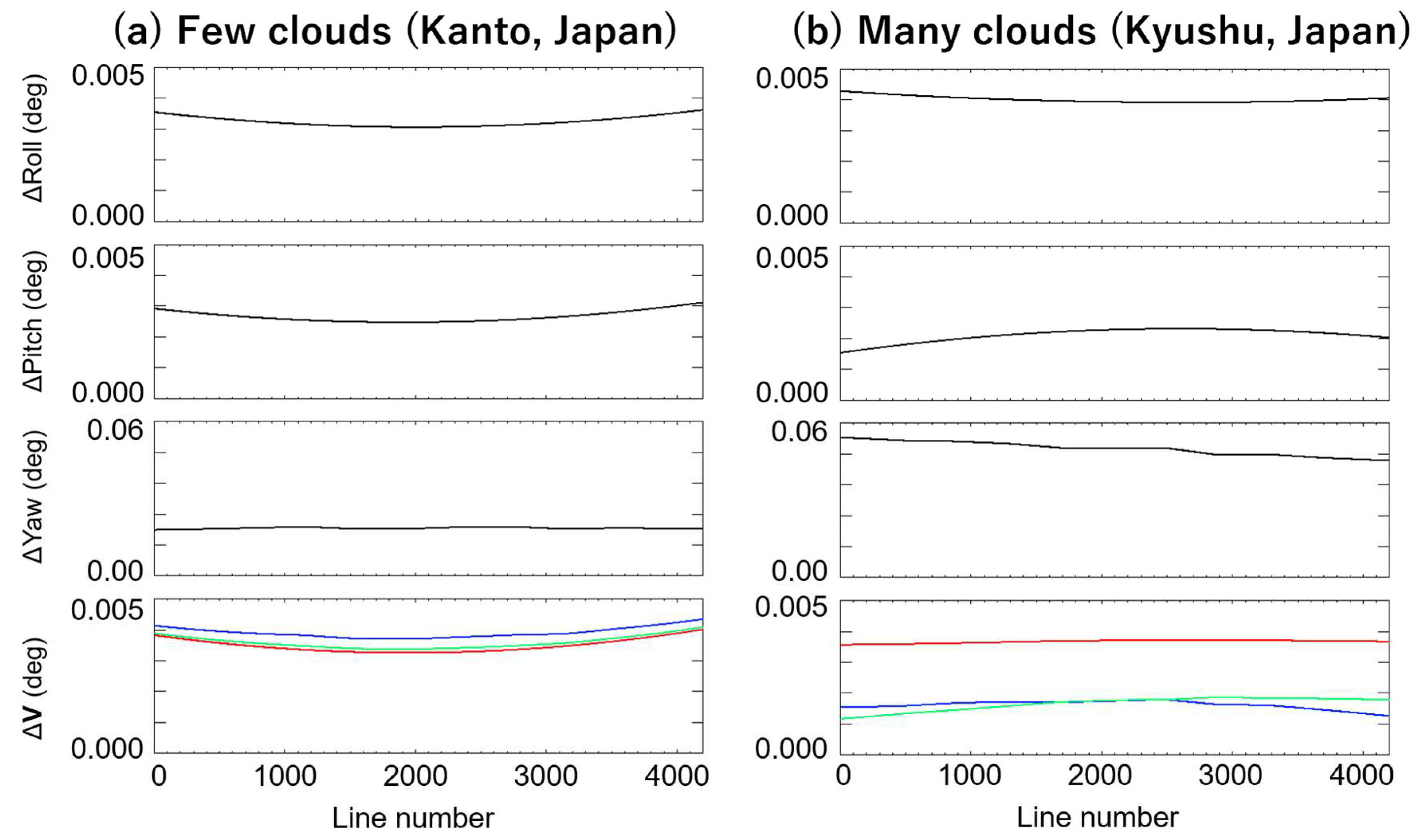
where indicates sensor attitude measured from the onboard attitude sensors of Terra/ASTER, such as STTs. Based on (7), roll, pitch, and yaw angles can be estimated from . Figure 7 shows the differences in the angles of the two attitudes. We also measured the differences in directions of line-of-sight vectors of the two attitudes, , at the center, the right and left edge pixels of the sensor which more directly relate to the difference in the map-projection results between the two attitudes.
The difference was around 0.003° in roll and pitch angles, and around 0.05° in yaw angle in both cases. Therefore, the proposed method successfully reproduced the temporal variation in ASTER sensor attitude.
4. Discussion
4.1. Performance of Attitude Determination in Extrapolated Areas
It is likely that a distribution of matched feature points covers only a limited part of a scene, and sensor attitude for parts of the images without feature points will be determined from “extrapolated” estimation. Since the bundle-adjustment approach adjusts parameters to fit only for the region where feature points exist, the accuracy of sensor attitude may decrease in the extrapolation area. On the other hand, attitude information in the extrapolated area should be important because accurate geometry information in sea areas is useful for many applications, such as ocean color analysis, monitoring sea surface temperature, and finding and preventing oil spreading. It is important to investigate the accuracy in sensor attitude in the extrapolation area.
To examine the accuracy in the extrapolation area, we derived sensor attitude with an ASTER scene (60 km southward of Figure 3b, Kyushu area) in which a large part of the scene was covered by sea and matched feature pairs were found in only the upper 1/4 of the ASTER scene (Figure 8a). From the comparison of sensor attitude derived from the proposed method with sensor attitude from STT, the difference in the attitudes obviously increased in the extrapolation area, which exceeded 0.1° in yaw angle at the bottom of the scene (Figure 8b) and exceeded 0.01° in directions of line-of-sight vectors at the center pixel of ASTER (Figure 8c). Since STT is expected to provide attitude with an accuracy of 0.01°, the derived attitude is incorrect in the extrapolation area. This large discrepancy derived by the proposed method is caused by the biased distribution of the matched features in a scene, though enough features (50 features) were able to be used for sensor-attitude determination.
Whereas one scene length of ASTER L1A is set to be almost the same as a scene width, one observation sequence of ASTER is usually much longer than the scene length of each ASTER level 1A product. When we examined sensor-attitude determination with matched features from three sequential scenes in which first two were land scenes and last one was almost a sea scene as in Figure 8a, then the derived attitude from the proposed method showed good consistency with the attitude value obtained from an STT in which at a center pixel showed less than 0.01° even in the extrapolation area (Figure 8c). We found the consistency (better than 0.01°) remained at ~90 km away from the coastline, and if we allow 0.02° difference in , then we can use the extrapolated area at the distance of 140 km. 0.02° error corresponds to just 250 m error on the ground in ASTER observations. In addition, our assumption of linear variation of sensor attitude is valid for at least three sequential observations of ASTER.
4.2. Design of Fitting Equations
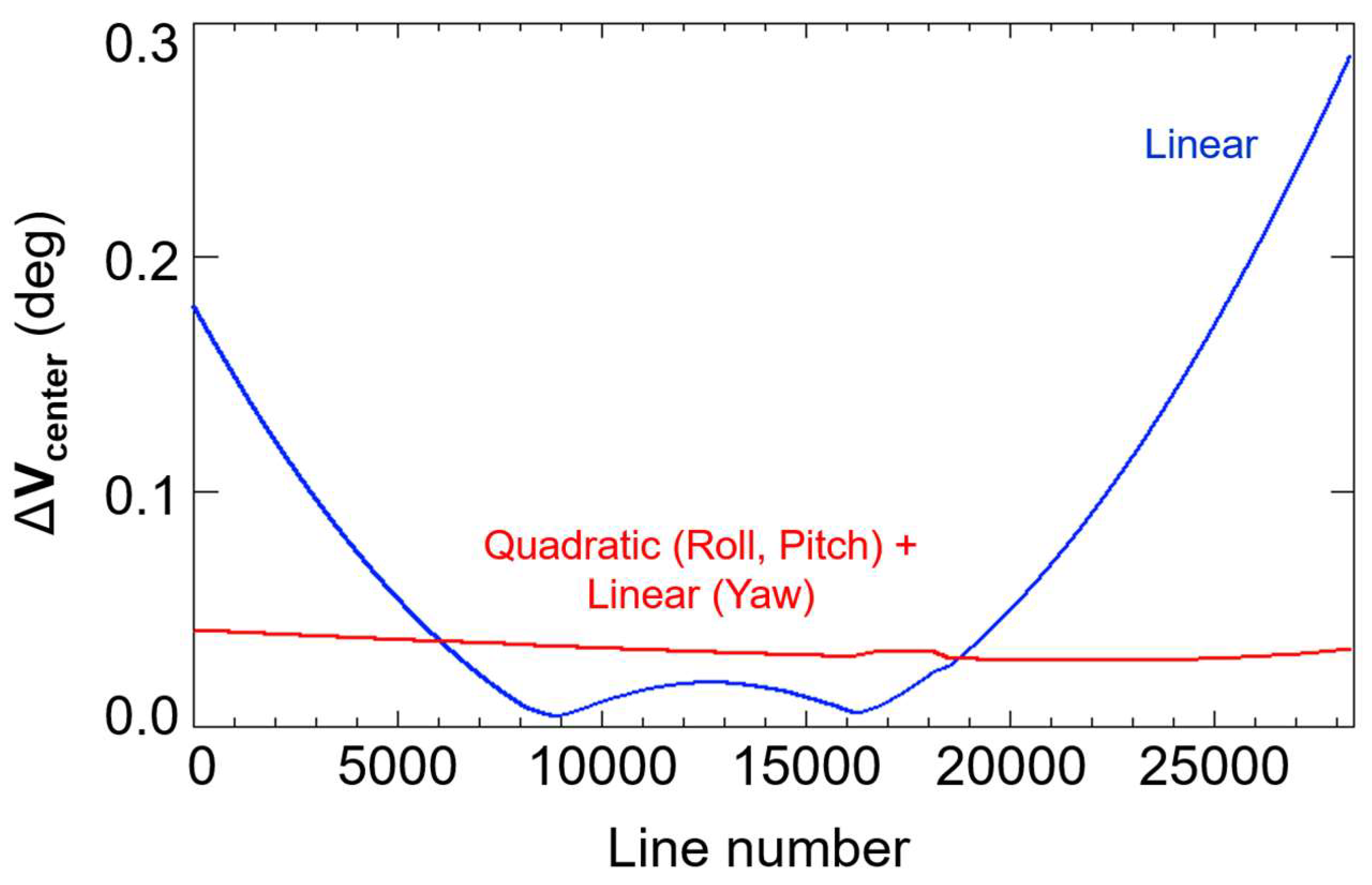
We introduced attitude determination with the linear equations in (8) for representing temporal variation in roll, pitch, and yaw angles from the view point of stable performance of the proposed method, and this assumption is valid for ASTER from one to at least three scene lengths. However, rather complicated attitude variation is possible depending on satellite operation. In fact, when we derived sensor attitude using feature points from seven scenes of ASTER, we found large systematic differences (more than 0.02°) in line-of-sight vector directions between the proposed method and using STTs (Figure 9). This means that temporal variation in ASTER attitude relative to the Earth is composed of not only constant rate variation but also time-dependent variation. To reduce the differences, we modified (8) to use quadratic functions for representing variations in roll and pitch angles instead of simple linear functions. As a result, the differences in line-of-sight vectors were successfully reduced to be less than 0.01°.
5. Conclusions
We developed an automated and robust method for deriving attitudes of a pushbroom sensor based on observed images with known satellite/sensor positions. By combining SURF and RANSAC-based algorithms at a rough estimation phase and using a non-linear least squares method at a precise estimation phase, the proposed scheme optimizes the solution under specific geometry conditions of a pushbroom sensor observation. The proposed method provides accurate satellite attitude independently of onboard attitude sensors including STTs. From experimental results using ASTER images, the proposed scheme achieved an accuracy of 0.003°, which is higher than that using STTs. The high accuracy derived by this method may contribute to validating and/or calibrating other onboard attitude sensors. It should be noted that the achieved accuracy may depend on the spatial resolution of a sensor.
The achieved accuracy of attitude determination will improve sensor operation such as for HISUI, which will be installed on the JEM of the ISS where sometimes STTs cannot be used. Even when no land features can be seen in large parts of a scene (e.g., cloud-covered images and sea observations), sensor attitude can be derived by extrapolating the derived temporal variation in sensor attitude from sequential observation scenes. Because of the low computational cost and stable performance, we recommend using only linear functions for the derivation of sensor attitude as a nominal procedure. In addition, the proposed method can be expanded to treat rather complicated temporal attitude variations by designing a fitting function appropriately for each satellite operation.
Author Contributions
T.K. and R.S. conceived and designed the study and wrote the paper; R.S designed and modified geometric fitting, conducted the experiments, and analyzed the data; T.K., A.K, S.K., and N.I. contributed materials; and R.S., T.K., and A.K., conceived of the discussion of accuracy of the proposed scheme.
Funding
This study was supported in part by the New Energy and Industrial Technology Development Organization (NEDO) and JSPS KAKENHI Grant Number 16H02225.
Acknowledgments
The authors thank USGS and JSS for the open data policy of ASTER and Landsat-8 mission. ASTER L1A images were obtained from https://lpdaac.usgs.gov, maintained by the NASA EOSDIS Land Processes Distributed Active Archive Center (LP DAAC) at the USGS/Earth Resources Observation and Science (EROS) Center, Sioux Falls, South Dakota. The ASTER data products for the image were produced by the NASA LP DAAC, the Japan Ministry of Economy, Trade and Industry (METI), Japan Space Systems, and Japan National Institute of Advanced Industrial Science and Technology (AIST). The authors thank Axelspace Corporation for their kind support for this study.
Conflicts of Interest
The authors declare no conflict of interest. The funding sponsors had no role in the design of the study, i.e., in the collection, analyses, or interpretation of data, writing of the manuscript, or in the decision to publish the results.
Appendix A
This section describes how to solve the non-linear least squares problem in (9) with iteration. By expressing the parameters estimated in a previous step with suffix o, the Taylor expansion of E can be written as
where
The notations are the coefficients of
and
where means the correction values of parameters for values estimated in a previous step. It is known that the minimized can be found by , which satisfies:
Based-on the idea from the Gaussian-Newton approach, (A5) can be solved with
where
Here, and are observed values. We will find minimized L and optimized parameters by repeating the above calculation until convergence by updating the center values of the Taylor expansion:
This scheme can be applicable in the same manner for
References
- Tahoun, M.; Shabayayek, A.E.R.; Hassanien, A.E. Matching and co-registration of satellite images using local features. In Proceedings of the International Conference on Space Optical Systems and Applications (ICSOS), Kobe, Japan, 7–9 May 2014. [Google Scholar]
- Wang, X.; Li, Y.; Wei, H.; Lin, F. An ASIFT-based local registration method for satellite imagery. Remote Sens. 2015, 7, 7044–7061. [Google Scholar] [CrossRef]
- Markley, F.H.; Crassidis, J.L. Sensors and Actuators. In Fundamentals of Spacecraft Attitude Determination and Control; Springer: Berlin, Germany, 2014; pp. 123–181. [Google Scholar]
- Matsunaga, T.; Iwasaki, A.; Tsuchida, S.; Iwao, K.; Tanii, J.; Kashimura, O.; Nakamura, R.; Yamamoto, H.; Kato, S.; Mouri, K.; et al. Current status of Hyperspectral Imager Suite (HISUI) onboard International Space Station (ISS). In Proceedings of the 2017 IEEE International Conference on Imaging Systems and Techniques, Beijing, China, 18–20 October 2017; IEEE: Fort Worth, TX, USA, 2017. [Google Scholar]
- Iwasaki, A.; Ohgi, N.; Tanii, J.; Kawashima, T.; Inada, H. Hyperspectral Imager Suite (HISUI) -Japanese hyper-multi spectral radiometer. In Proceedings of the 2011 IEEE International Geoscience and Remote Sensing Symposium, Vancouver, BC, Canada, 24–29 July 2011; pp. 1025–1028. [Google Scholar] [CrossRef]
- Belyaev, M.Y.; Babkin, E.V.; Ryabukha, S.B.; Ryazantsev, A.V. Microperturbations on the International Space Station during physical exercises of the crew. Cosm. Res. 2011, 49, 160. [Google Scholar] [CrossRef]
- Morii, M.; Sugimori, K.; Kawai, N.; The Maxi team. Alignment calibration of MAXI/GSC. Physica E 2011, 43, 692–696. [Google Scholar] [CrossRef]
- Kibo Exposed Facility User Handbook. Available online: http://iss.jaxa.jp/kibo/library/fact/data/JFE_HDBK_all_E.pdf (accessed on 13 April 2018).
- Kouyama, T.; Kanemura, A.; Kato, S.; Imamoglu, N.; Fukuhara, T.; Nakamura, R. Satellite Attitude Determination and Map Projection Based on Robust Image Matching. Remote Sens. 2017, 9, 90. [Google Scholar] [CrossRef]
- Brum, A.G.V.; Pilchowski, H.U.; Faria, S.D. Attitude determination of spacecraft with use of surface imaging. In Proceedings of the 9th Brazilian Conference on Dynamics Control and Their Applications (DICON’10), Serra Negra, Brazil, 7–11 June 2010; pp. 1205–1212. [Google Scholar]
- Barbieux, K. Pushbroom Hyperspectral Data Orientation by Combining Feature-Based and Area-Based Co-Registration Techniques. Remote Sens. 2018, 10, 645. [Google Scholar] [CrossRef]
- Toutin, T. Review article: Geometric processing of remote sensing images: Models, algorithms and methods. Int. J. Remote Sens. 2004, 25, 1893–1924. [Google Scholar] [CrossRef]
- Poli, D. General Model for Airborne and Spaceborne Linear Array Sensors. Int. Arch. Photogramm. Remote Sens. Spat. Inf. Sci. 2002, 34, 177–182. [Google Scholar]
- Poli, D.; Zhang, L.; Gruen, A. Orientation of satellite and airborne imagery from multi-line pushbroom sensors with a rigorous sensor model. Int. Arch. Photogramm. Remote Sens. Spat. Inf. Sci. 2004, 35, 130–135. [Google Scholar]
- Aguilar, M.A.; Saldana, M.M.; Aguilar, F.J. Assessing geometric accuracy of the orthorectification process from GeoEye-1 and WorldView-2 panchromatic images. Int. J. Appl. Earth Obs. Geoinf. 2013, 21, 427–435. [Google Scholar] [CrossRef]
- Bay, H.; Ess, A.; Tuytelaars, T.; Gool, L.V. Speeded-up robust features (SURF). Comput. Vis. Image Underst. 2008, 110, 346–359. [Google Scholar] [CrossRef]
- Fisher, M.A.; Bolles, R.C. Random sample consensus: A paradigm for model fitting with applications to image analysis and automated cartography. Commun. ACM 1981, 24, 381–395. [Google Scholar]
- Choi, S.; Kim, T.; Yu, W. Performance Evaluation of RANSAC Family. In Proceedings of the British Machine Vision Conference 2009, London, UK, 7–10 September 2009. [Google Scholar]
- Triggs, B.; McLauchlan, P.; Hartley, R.; Fitzgibbon, A. Bundle Adjustment—A Modern Synthesis. In Vision Algorithms: Theory and Practice, Proceedings of the International Workshop on Vision Algorithms: Theory and Practice, Corfu, Greece, 20–25 September 1999; Springer: London, UK, 1999; pp. 298–372. ISBN 3-540-67973-1. [Google Scholar]
- Jing, L.; Xu, L.; Li, X.; Tian, X. Determination of Platform Attitude through SURF Based Aerial Image Matching. In Proceedings of the 2013 IEEE International Conference on Imaging Systems and Techniques, Beijing, China, 22–23 October 2013. [Google Scholar]
- Bradski, G.; Kaehler, A. Learning OpenCV: Computer Vision with the OpenCV Library; O’Reilly Media: Sebastopol, CA, USA, 2008; pp. 521–526. [Google Scholar]
- Chum, O.; Matas, J. Matching with PROSAC—Progressive Sample Consensus. In Proceedings of the International Conference on Computer Vision and Pattern Recognition, San Diego, CA, USA, 20–26 June 2005. [Google Scholar]
- Aster Overview. Available online: https://lpdaac.usgs.gov/dataset_discovery/aster (accessed on 13 April 2018).
- Keiffer, H.H.; Mullin, K.F.; MacKinnon, D.J. Validation of the ASTER Instrument Level 1A Scene Geometry. Photogramm. Eng. Remote Sens. 2008, 74, 289–301. [Google Scholar] [CrossRef]
- Kelly, A.; Moyera, E.; Mantziarasa, D.; Caseb, W. Terra mission operations: Launch to the present (and beyond). In Proceedings of the SPIE, Earth Observing Systems, San Diego, CA, USA, 17–21 August 2014. [Google Scholar]
- Ward, D.; Dang, K.; Slojkowski, S.; Blizzard, M.; Jenkins, G. Tracking and Data Relay Satellite (TDRS) Orbit Estimation Using an Extended Kalman Filter. In Proceedings of the 20th International Symposium on Space Flight Dynamics, Annapolis, MD, USA, 24–28 September 2007. [Google Scholar]
- Strorey, J.; Choate, M.; Lee, K. Landsat 8 operational land imager on-orbit geometric calibration and performance. Remote Sens. 2014, 6, 11127–11152. [Google Scholar] [CrossRef]
- ASTER GDEM Validation Team. ASTER Global Digital Elevation Model Version 2—Summary of Validation Results 2011. Available online: http://www.jspacesystems.or.jp/ersdac/GDEM/ver2Validation/Summary_GDEM2_validation_report_final.pdf (accessed on 8 August 2016).
- Athmania, D.; Achour, H. External validation of the ASTER GDEM2, GMTED2010 and CGIAR-CSI- SRTM v4.1 free access digital elevation models (DEMs) in Tunisia and Algeria. Remote Sens. 2014, 6, 4600–4620. [Google Scholar] [CrossRef]
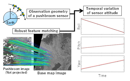
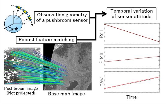
Figure 1.
Overview of proposed method for satellite attitude determination based on pushbroom (not projected) and base-map images. The method consists of three major steps; feature extraction, outlier elimination and rough attitude estimation, and precise attitude estimation.
Figure 1.
Overview of proposed method for satellite attitude determination based on pushbroom (not projected) and base-map images. The method consists of three major steps; feature extraction, outlier elimination and rough attitude estimation, and precise attitude estimation.

Figure 2.
Schematic views of (a) ; and (b) . is point on Earth’s surface where land feature has been detected at scan time , and is its projected point on detector plane. i, j, and h indicate different lines in observation sequence.
Figure 2.
Schematic views of (a) ; and (b) . is point on Earth’s surface where land feature has been detected at scan time , and is its projected point on detector plane. i, j, and h indicate different lines in observation sequence.
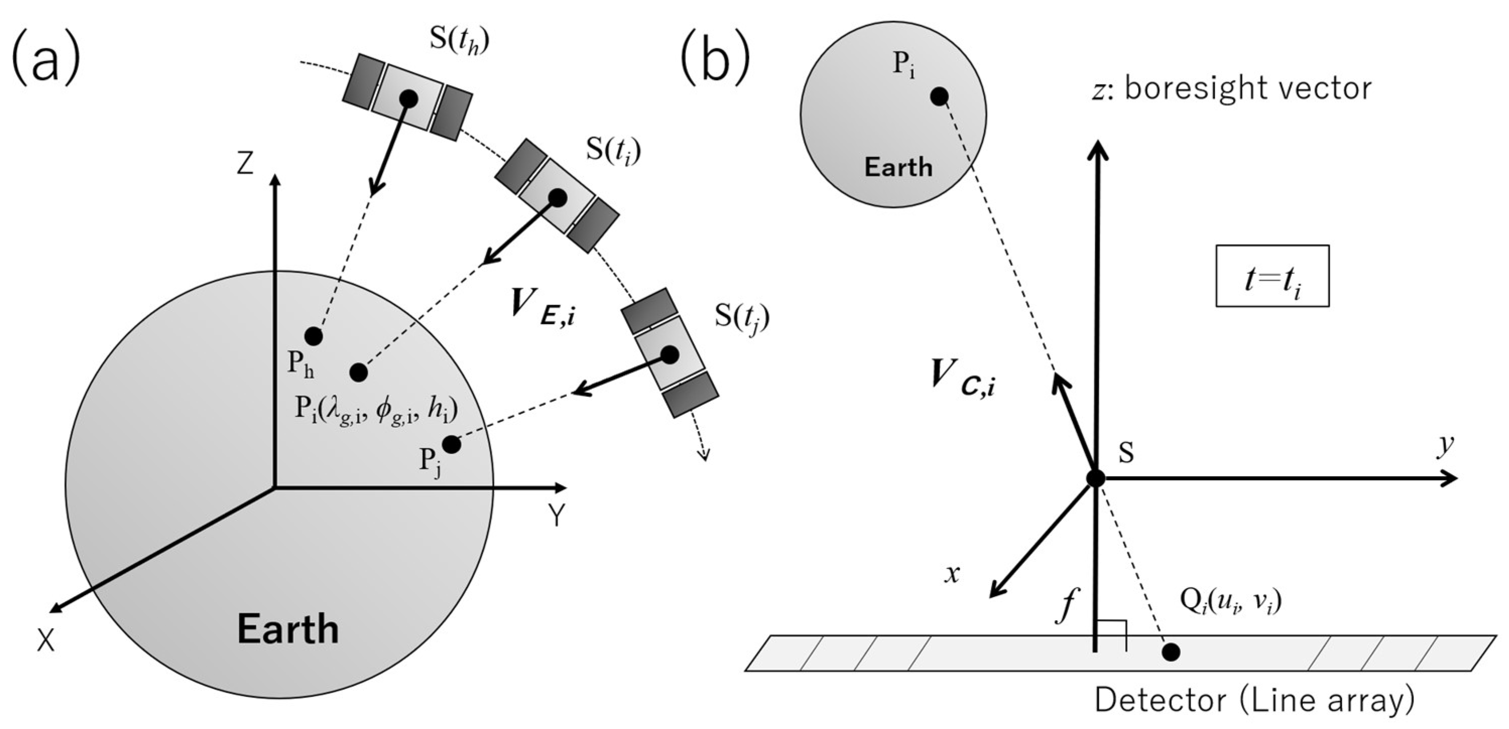
Figure 3.
Examples of feature extraction and rough matching for (a) few clouds (Kanto, Japan) and (b) many clouds (Kyushu, Japan) by using SURF algorithm, which includes both correctly and incorrectly matched pairs. Left and right panels are raw image from ASTER observation and map-projected image from Landsat OLI, respectively. “+” represent locations of detected SURF features, and lines connect pairs of corresponding features in two images. Line color represents relative similarity of paired features (blue to red in order of increasing similarity) measured as distance of SURF descriptors between these features.

Figure 4.
Same as Figure 3 but eliminating incorrectly matched pairs based on a robust feature-matching method [9].

Figure 5.
Derived temporal variations of ASTER attitude (roll, pitch, and yaw angles) during observations for cases of (a) few clouds and (b) many clouds in Figure 4. Solid lines indicate sensor attitude measured from proposed method and dashed lines are from onboard attitude sensors of ASTER.
Figure 5.
Derived temporal variations of ASTER attitude (roll, pitch, and yaw angles) during observations for cases of (a) few clouds and (b) many clouds in Figure 4. Solid lines indicate sensor attitude measured from proposed method and dashed lines are from onboard attitude sensors of ASTER.

Figure 6.
Examples of map-projected ASTER images and their zoom-in images based on sensor attitude deduced from proposed method for scenes with (a) few clouds and (b) many clouds.
Figure 6.
Examples of map-projected ASTER images and their zoom-in images based on sensor attitude deduced from proposed method for scenes with (a) few clouds and (b) many clouds.
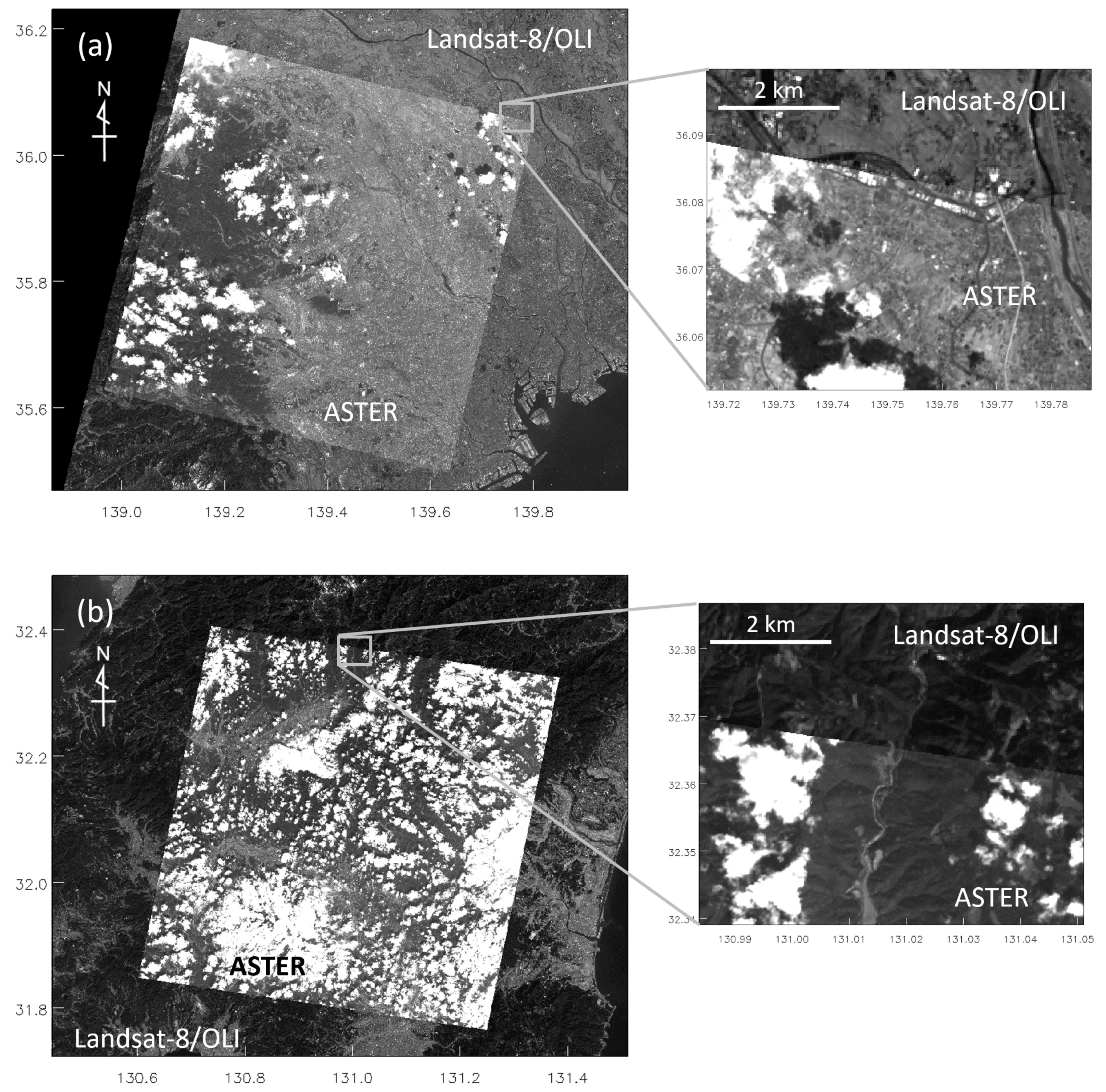
Figure 7.
Differences of roll, pitch and yaw angles between two attitudes derived from onboard attitude sensors of Terra/ASTER and proposed method in (a) few clouds and (b) many clouds. Bottom panels show differences in directions of line-of-sight vectors between two attitudes at center (red line), left edge (green), and right edge (blue lines) of ASTER in each line.

Figure 8.
(a) ASTER L1A scene in which large part of scene was covered by sea. “+” denotes locations of matched features used for attitude determination. (b) Comparison of yaw angles derived from the proposed method using only one scene (blue solid), and sequential three scenes (red solid), and derived from onboard attitude sensors (dashed). (c) Differences in directions of line-of-sight vectors at the center pixel of ASTER between two attitudes derived from onboard attitude sensors and the proposed method using only one scene (blue line) and sequential three scenes (red line).
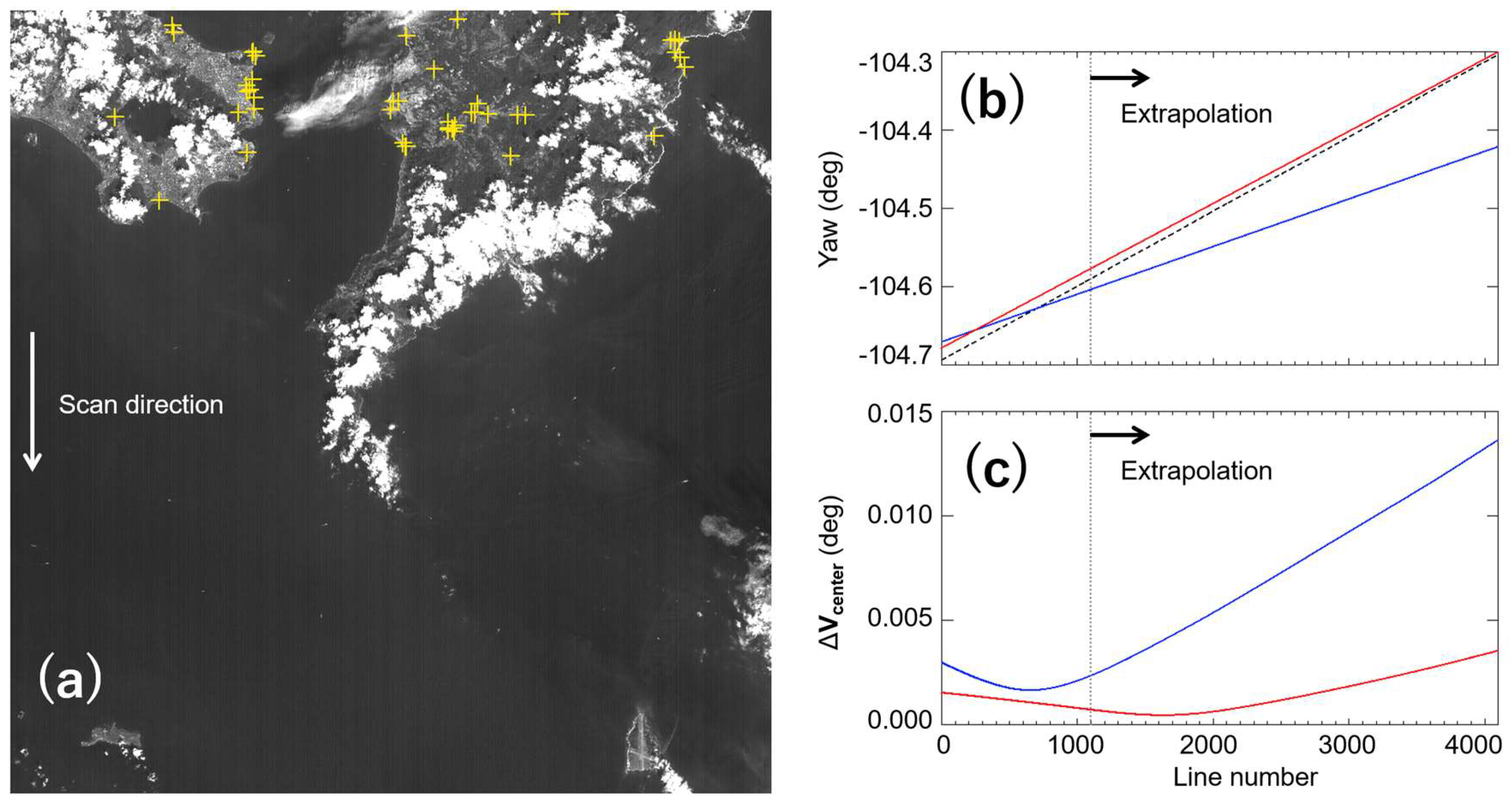
Figure 9.
Temporal variations of differences in directions of line-of-sight vectors at the center of ASTER derived from onboard sensors and the proposed method in sequential observations (composed of seven scenes). The blue line shows the result from using only linear equations and the red line is from combining linear and quadric equations.

Table 1.
Specifications of ASTER Band 1 onboard Terra.
| Wavelength (μm) | GSD (m) | Swath (km) | Bit Depth (bit) | |
|---|---|---|---|---|
| ASTER Band 1 | 0.52–0.60 | 15 | 60 | 8 |
Table 2.
Specifications of base-map image of OLI (Band 3) onboard Landsat-8.
| Wavelength (μm) | GSD (m) | Swath (km) | Bit Depth (bit) | |
|---|---|---|---|---|
| OLI Band 3 | 0.533–0.590 | 30 | 185 | 16 |
Table 3.
Mean miss-registration errors and RMSEs of matched feature pairs extracted from projected ASTER and OLI images. The projection was examined based on sensor attitude from onboard sensors and proposed method for comparison. Symbols and represent east–west and north–south directions, respectively.
| Onboard Sensors | Proposed | |||||||
|---|---|---|---|---|---|---|---|---|
| (a) Kanto, Japan (Few clouds) | −3.1 | −2.1 | 15.5 | 12.0 | −3.8 | −2.1 | 14.4 | 13.2 |
| (b) Kyushu, Japan (Many clouds) | −20 | −5.1 | 15.0 | 13.0 | −5.2 | −5.6 | 11.7 | 13.8 |
© 2018 by the authors. Licensee MDPI, Basel, Switzerland. This article is an open access article distributed under the terms and conditions of the Creative Commons Attribution (CC BY) license (http://creativecommons.org/licenses/by/4.0/).
Share and Cite
MDPI and ACS Style
Sugimoto, R.; Kouyama, T.; Kanemura, A.; Kato, S.; Imamoglu, N.; Nakamura, R. Automated Attitude Determination for Pushbroom Sensors Based on Robust Image Matching. Remote Sens. 2018, 10, 1629. https://doi.org/10.3390/rs10101629
AMA Style
Sugimoto R, Kouyama T, Kanemura A, Kato S, Imamoglu N, Nakamura R. Automated Attitude Determination for Pushbroom Sensors Based on Robust Image Matching. Remote Sensing. 2018; 10(10):1629. https://doi.org/10.3390/rs10101629
Chicago/Turabian StyleSugimoto, Ryu, Toru Kouyama, Atsunori Kanemura, Soushi Kato, Nevrez Imamoglu, and Ryosuke Nakamura. 2018. "Automated Attitude Determination for Pushbroom Sensors Based on Robust Image Matching" Remote Sensing 10, no. 10: 1629. https://doi.org/10.3390/rs10101629
Note that from the first issue of 2016, this journal uses article numbers instead of page numbers. See further details here.