Semi-Automated Delineation of Stands in an Even-Age Dominated Forest: A LiDAR-GEOBIA Two-Stage Evaluation Strategy


Abstract
1. Introduction
2. Materials
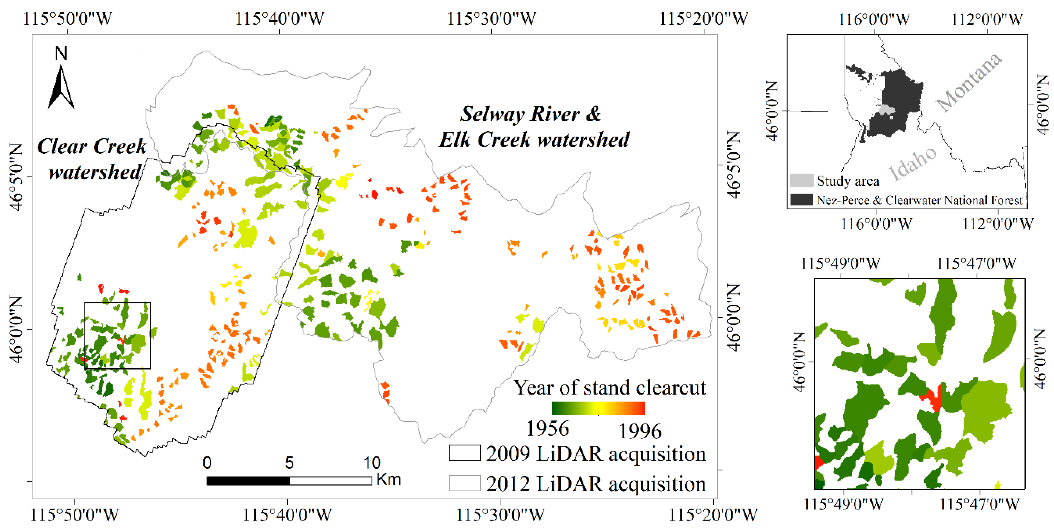
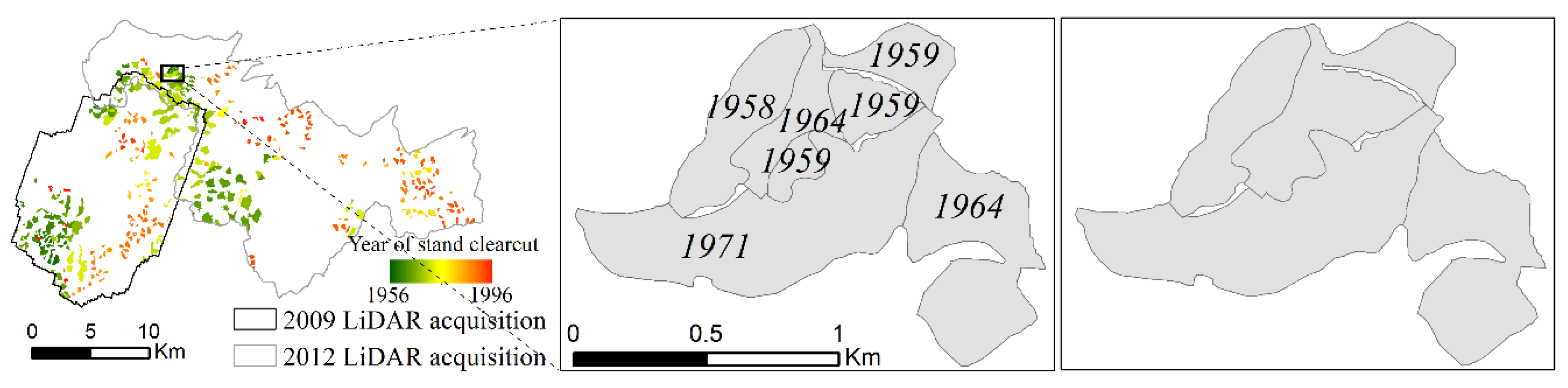
2.1. Study Area
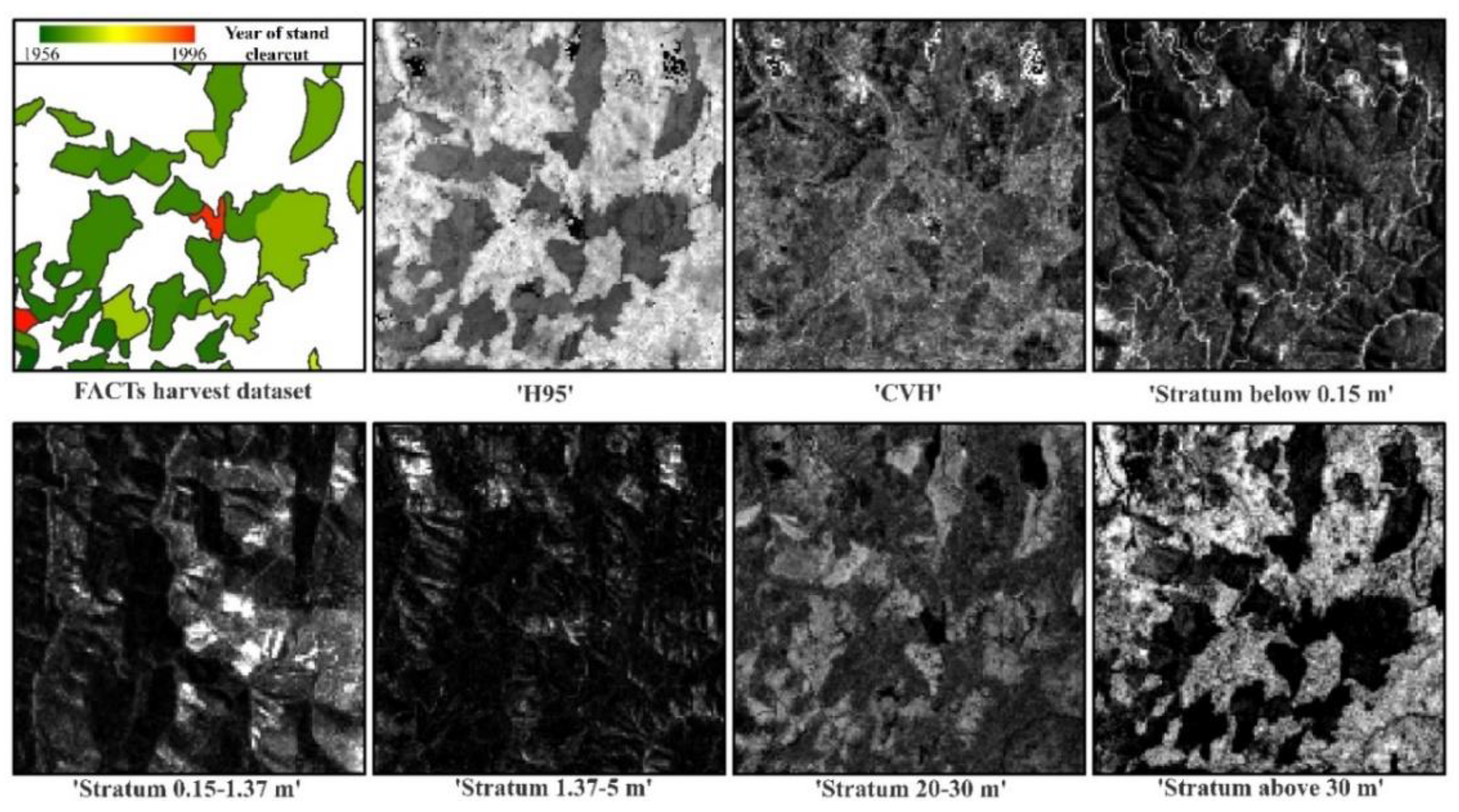
2.2. Ancillary Reference Data and Pre-Processing
2.3. LiDAR Datasets and Data Pre-Processing
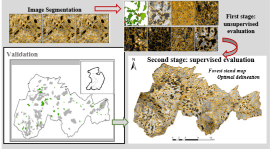
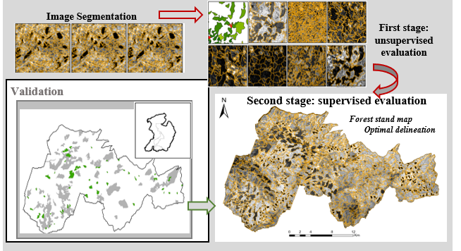
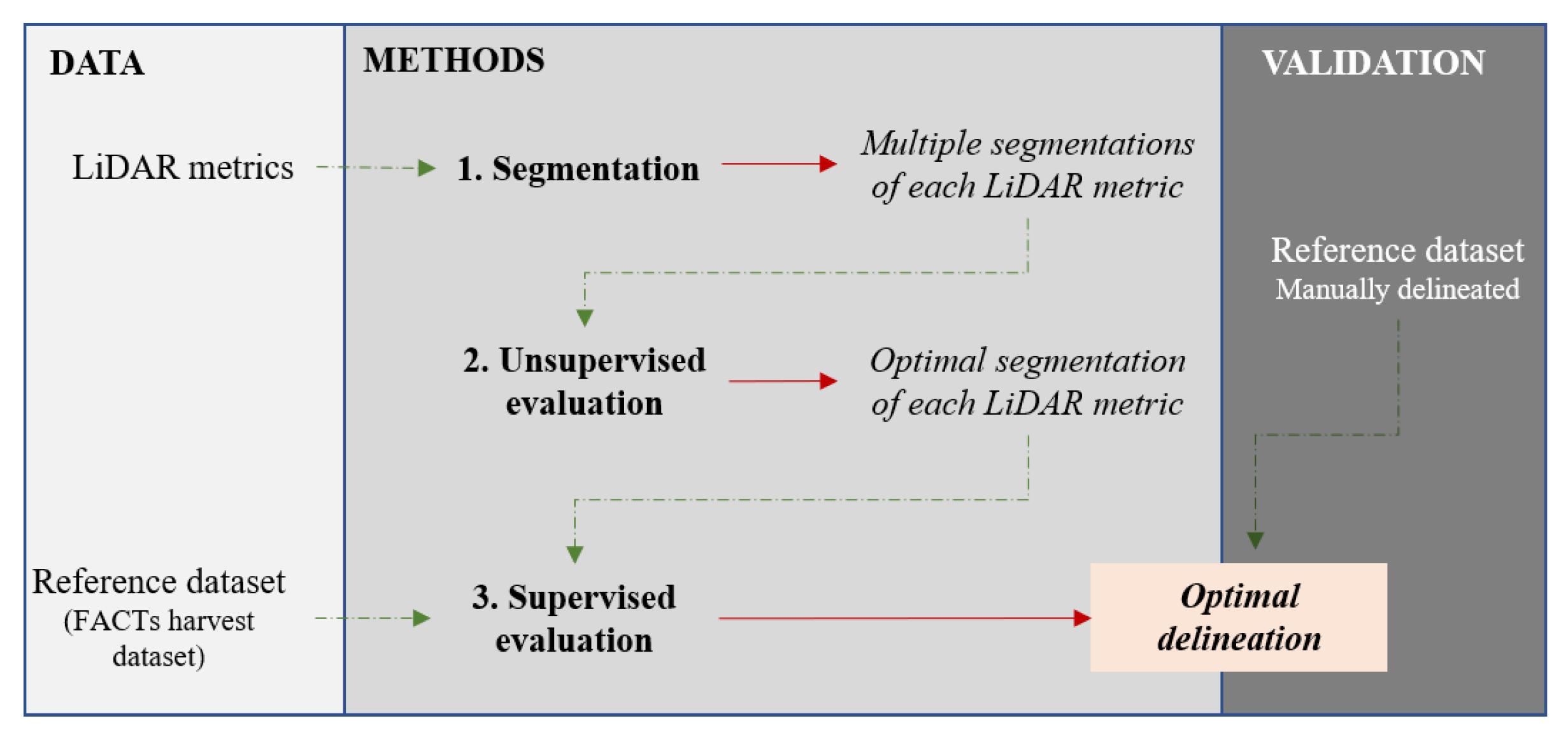
3. Methods
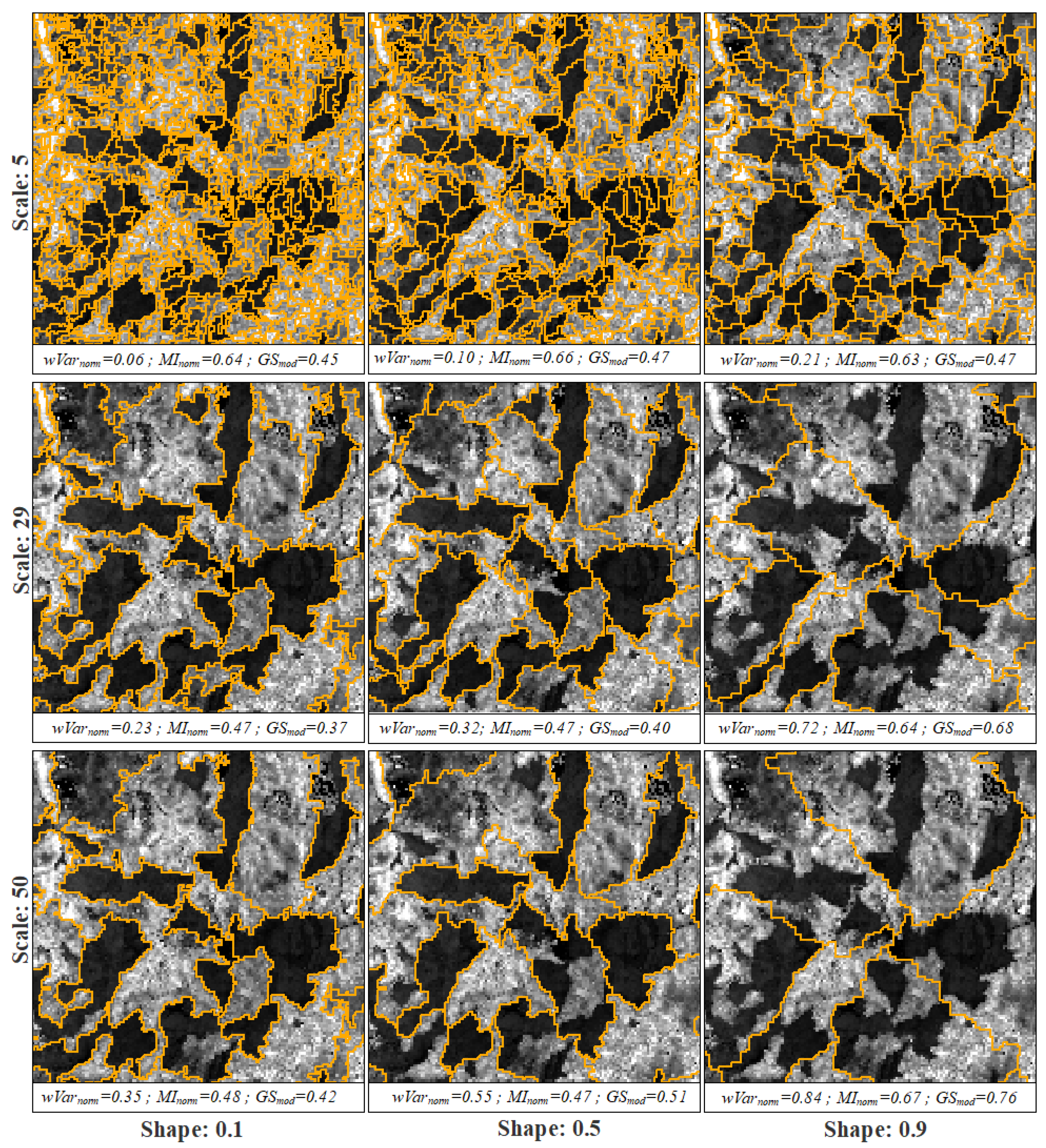
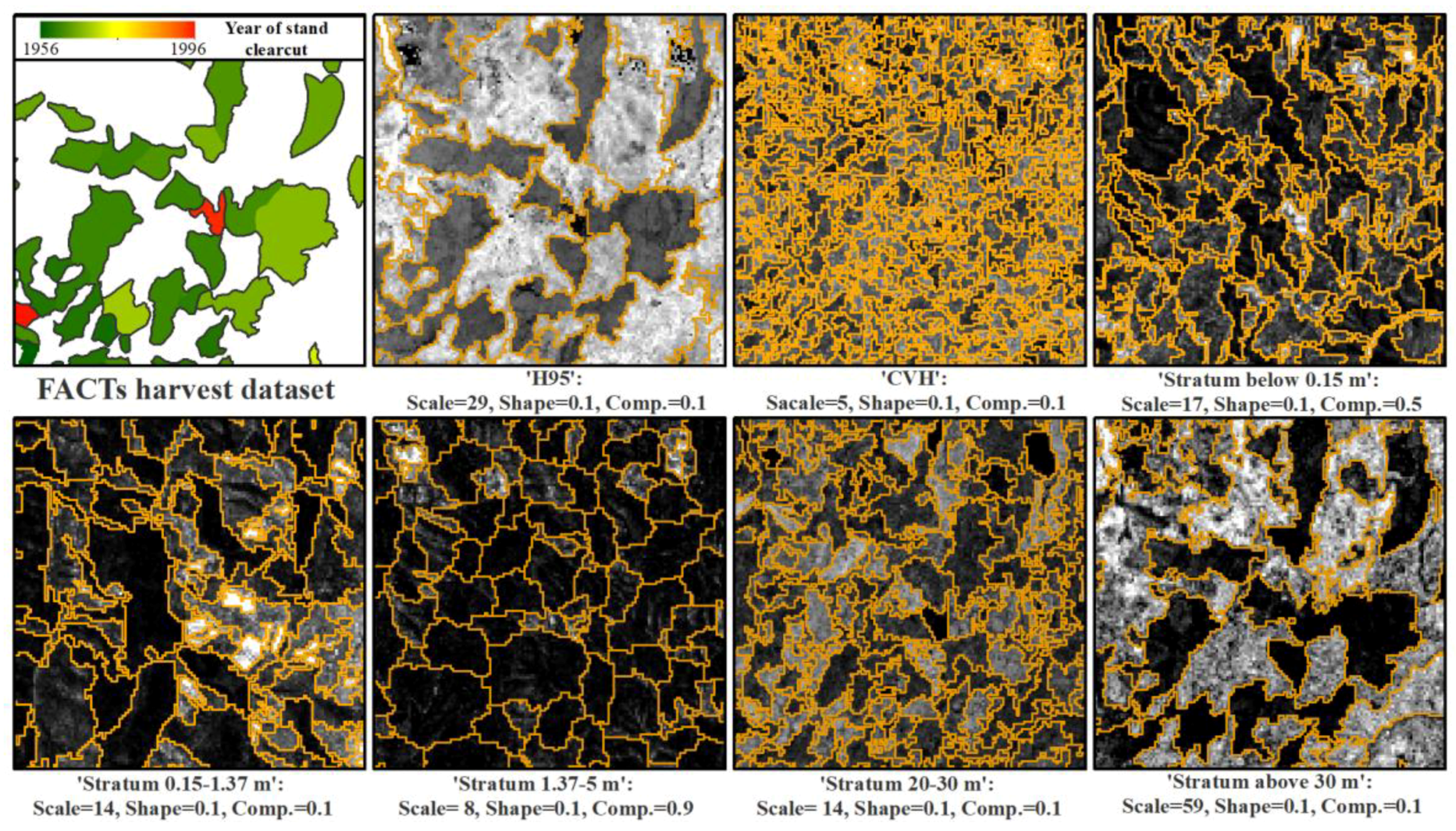
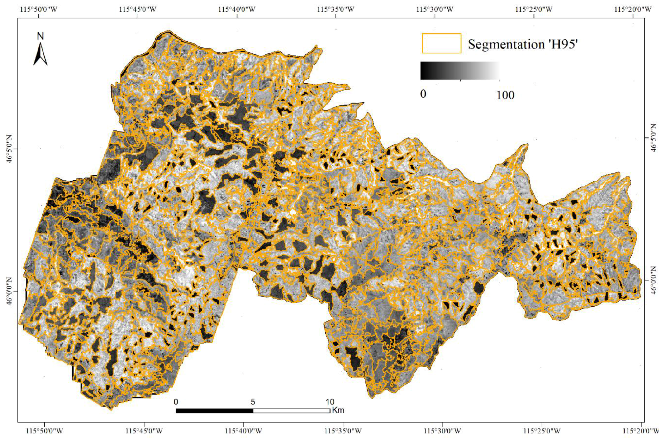
3.1. Segmentation
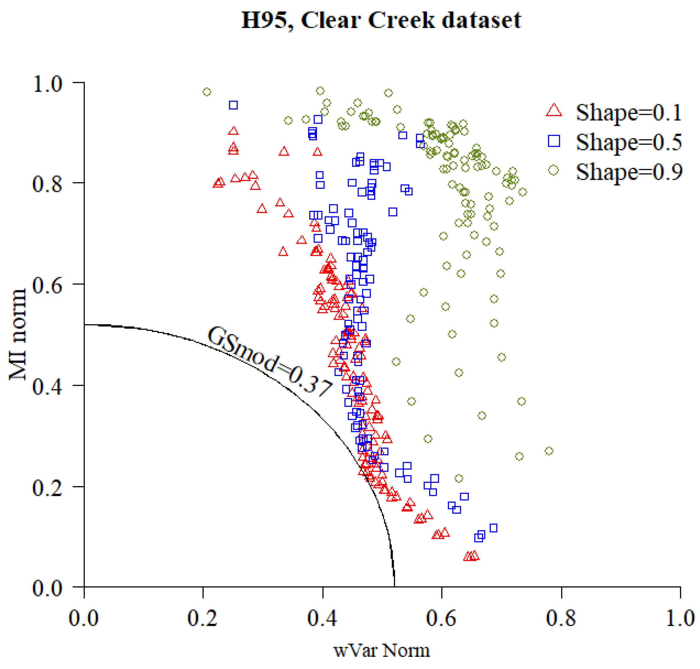
3.2. Selection of the Optimal Segmentation of each LiDAR Metric
3.3. Selection of the Optimal LiDAR Metric
- All clearcuts (years from 1956 to 1996);
- clearcuts performed before the start of the Landsat MSS record (years from 1956 to 1972);
- clearcuts performed before the start of the Landsat TM record (years from 1956 to 1984);
- clearcuts performed after the start of the Landsat TM record (years from 1984 to 1996).
3.4. Validation
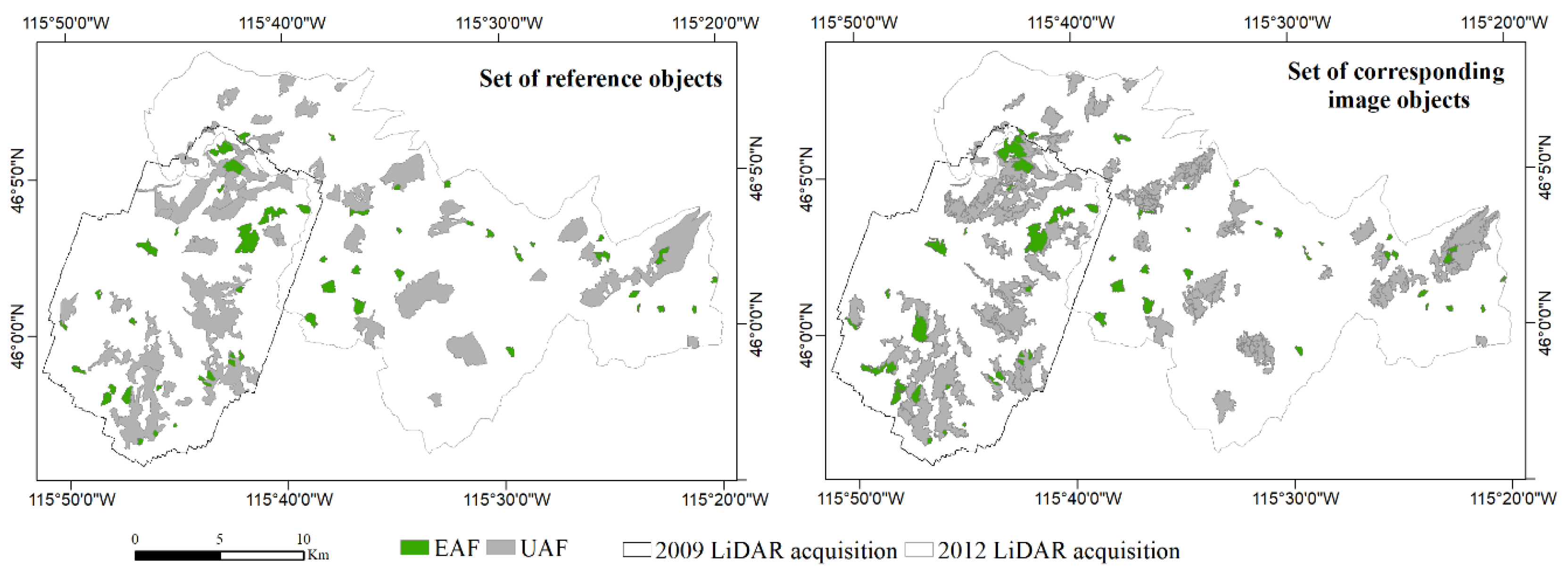
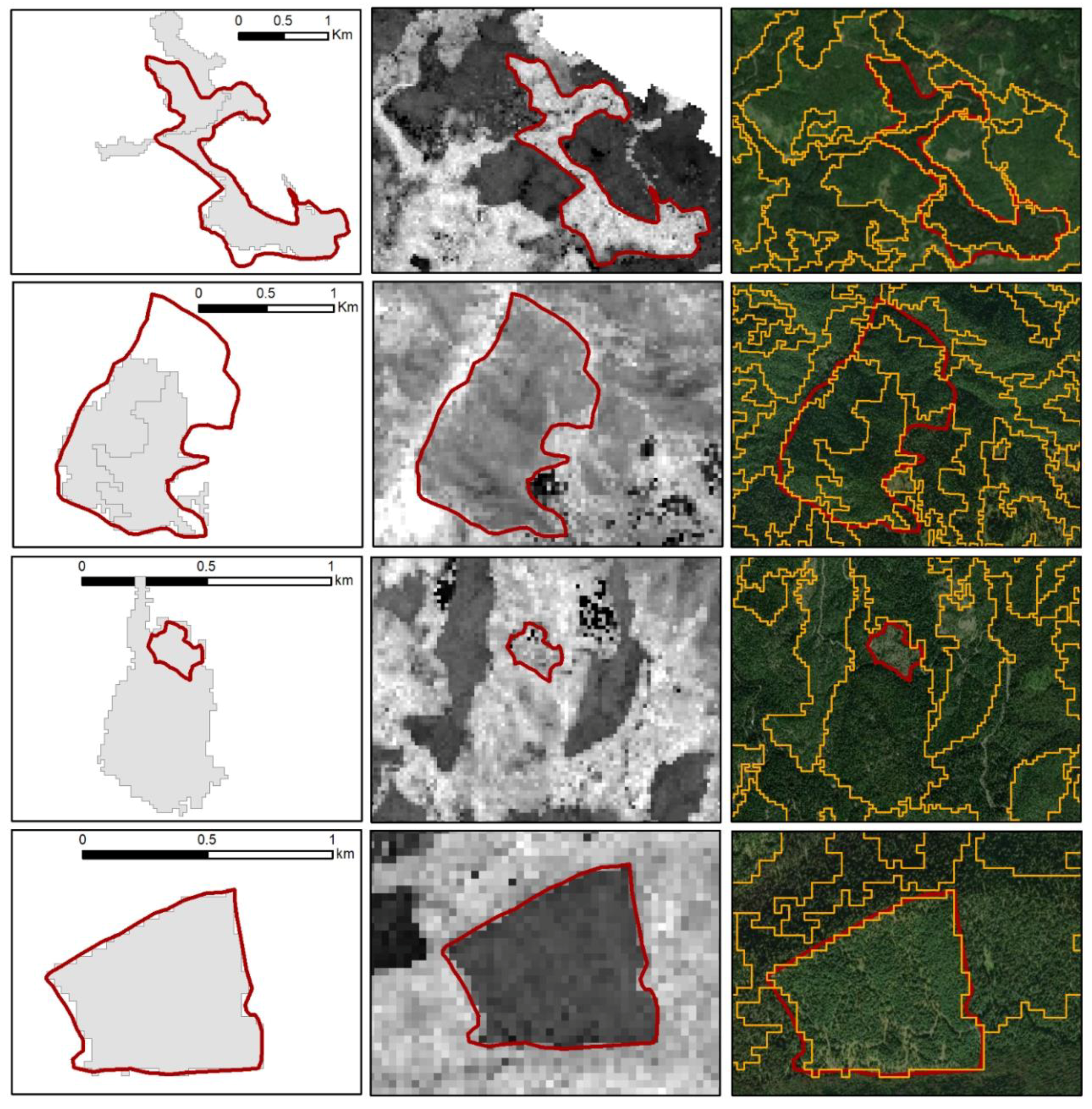
3.4.1. Reference Dataset
- Random selection of an image object of the optimal segmentation, to account for the large disparity in stand area, followed by random selection of a point within the object [60];
- visual interpretation of the NAIP imagery to trace the forest stand that includes the point. Any physical barriers such as roads or watersheds were used to delineate the border of the stands when no other natural discontinuity related to vegetation type or structure was found;
- classification of the reference object as EAF or uneven-aged forest by the photo-interpreter.
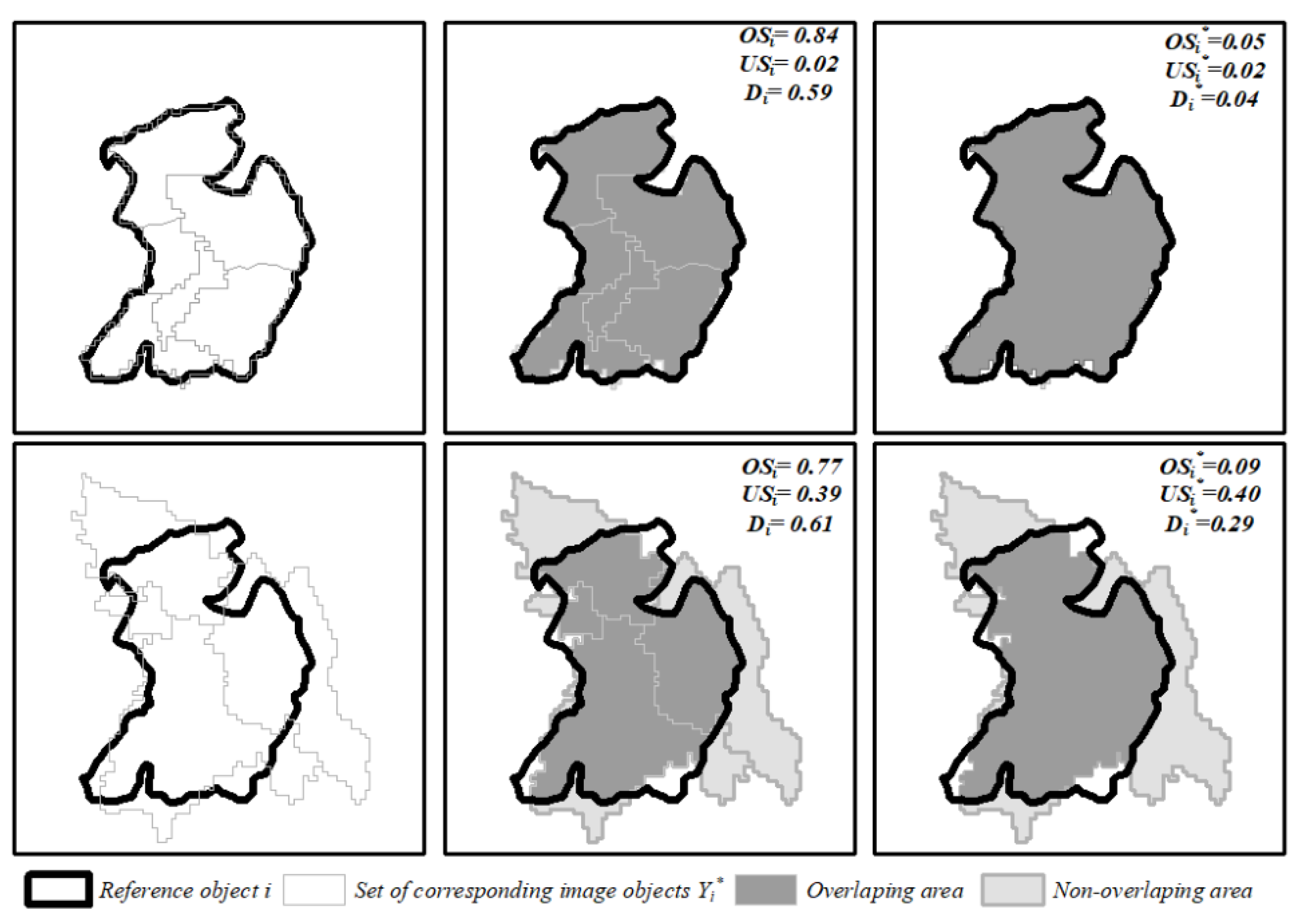
3.4.2. Validation Metrics
- Oversegmentation (OS), undersegmentation (US) and summary score (D), obtained with the procedure described in Section 4.3;
- modified oversegmentation (), undersegmentation (), and summary score (), defined as follows.
4. Results
4.1. Selection of the Optimal Segmentation of each LiDAR Metric
4.2. Selection of the Optimal LiDAR Metric
4.3. Validation
5. Discussion
6. Conclusions
Author Contributions
Funding
Conflicts of Interest
References
- Leckie, D.G.; Gougeon, F.A.; Walsworth, N.; Paradine, D. Stand delineation and composition estimation using semi-automated individual tree crown analysis. Remote Sens. Environ. 2003, 85, 355–369. [Google Scholar] [CrossRef]
- Sullivan, A.A.; McGaughey, R.J.; Andersen, H.-E.; Schiess, P. Object-oriented classification of forest structure from light detection and ranging data for stand mapping. West. J. Appl. For. 2009, 24, 198–204. [Google Scholar]
- Helms, J. The Dictionary of Forestry; Western Heritage Co.: Loveland, CO, USA, 1998. [Google Scholar]
- Masek, J.G.; Goward, S.N.; Kennedy, R.E.; Cohen, W.B.; Moisen, G.G.; Schleeweis, K.; Huang, C. United States Forest Disturbance Trends Observed Using Landsat Time Series. Ecosystems 2013, 16, 1087–1104. [Google Scholar] [CrossRef]
- White, J.C.; Wulder, M.A.; Hermosilla, T.; Coops, N.C.; Hobart, G.W. A nationwide annual characterization of 25 years of forest disturbance and recovery for Canada using Landsat time series. Remote Sens. Environ. 2017, 194, 303–321. [Google Scholar] [CrossRef]
- Leckie, D.G.; Gillis, M.D. Forest inventory in Canada with emphasis on map production. For. Chron. 1995, 71, 74–88. [Google Scholar] [CrossRef]
- Fisher, R.A.; Koven, C.D.; Anderegg, W.R.; Christoffersen, B.O.; Dietze, M.C.; Farrior, C.E.; Holm, J.A.; Hurtt, G.C.; Knox, R.G.; Lawrence, P.J. Vegetation demographics in Earth System Models: A review of progress and priorities. Glob. Chang. Biol. 2018, 24, 35–54. [Google Scholar] [CrossRef] [PubMed]
- Burnett, C.; Blaschke, T. A multi-scale segmentation/object relationship modelling methodology for landscape analysis. Ecol. Model. 2003, 168, 233–249. [Google Scholar] [CrossRef]
- Dechesne, C.; Mallet, C.; Le Bris, A.; Gouet-Brunet, V. Semantic segmentation of forest stands of pure species combining airborne lidar data and very high resolution multispectral imagery. ISPRS J. Photogramm. Remote Sens. 2017, 126, 129–145. [Google Scholar] [CrossRef]
- Koch, B.; Straub, C.; Dees, M.; Wang, Y.; Weinacker, H. Airborne laser data for stand delineation and information extraction. Int. J. Remote Sens. 2009, 30, 935–963. [Google Scholar] [CrossRef]
- Pascual, C.; García-Abril, A.; García-Montero, L.G.; Martín-Fernández, S.; Cohen, W.B. Object-based semi-automatic approach for forest structure characterization using lidar data in heterogeneous Pinus sylvestris stands. For. Ecol. Manag. 2008, 255, 3677–3685. [Google Scholar] [CrossRef]
- Tiede, D.; Blaschke, T.; Heurich, M. Object-based semi automatic mapping of forest stands with Laser scanner and Multi-spectral data. Int. Arch. Photogramm. Remote Sens. Spat. Inf. Sci. 2004, 36, 328–333. [Google Scholar]
- Wulder, M.A.; White, J.C.; Hay, G.J.; Castilla, G. Towards automated segmentation of forest inventory polygons on high spatial resolution satellite imagery. For. Chron. 2008, 84, 221–230. [Google Scholar] [CrossRef]
- Blaschke, T.; Lang, S.; Hay, G. Object-Based Image Analysis: Spatial Concepts for Knowledge-Driven Remote Sensing Applications; Springer Science & Business Media: Berlin, Germany, 2008; ISBN 978-3-540-77058-9. [Google Scholar]
- Blaschke, T.; Hay, G.J.; Kelly, M.; Lang, S.; Hofmann, P.; Addink, E.; Queiroz Feitosa, R.; van der Meer, F.; van der Werff, H.; van Coillie, F.; et al. Geographic Object-Based Image Analysis—Towards a new paradigm. ISPRS J. Photogramm. Remote Sens. 2014, 87, 180–191. [Google Scholar] [CrossRef] [PubMed]
- Costa, H.; Foody, G.M.; Boyd, D.S. Supervised methods of image segmentation accuracy assessment in land cover mapping. Remote Sens. Environ. 2018, 205, 338–351. [Google Scholar] [CrossRef]
- Liu, D.; Xia, F. Assessing object-based classification: Advantages and limitations. Remote Sens. Lett. 2010, 1, 187–194. [Google Scholar] [CrossRef]
- Walter, V. Object-based classification of remote sensing data for change detection. ISPRS J. Photogramm. Remote Sens. 2004, 58, 225–238. [Google Scholar] [CrossRef]
- Zhang, Y.J. A survey on evaluation methods for image segmentation. Pattern Recognit. 1996, 29, 1335–1346. [Google Scholar] [CrossRef]
- Belgiu, M.; Drǎguţ, L. Comparing supervised and unsupervised multiresolution segmentation approaches for extracting buildings from very high resolution imagery. ISPRS J. Photogramm. Remote Sens. 2014, 96, 67–75. [Google Scholar] [CrossRef] [PubMed]
- Clinton, N.; Holt, A.; Scarborough, J.; Yan, L.I.; Gong, P. Accuracy assessment measures for object-based image segmentation goodness. Photogramm. Eng. Remote Sens. 2010, 76, 289–299. [Google Scholar] [CrossRef]
- Neubert, M.; Herold, H.; Meinel, G. Assessing image segmentation quality—Concepts, methods and application. In Object-Based Image Analysis; Blaschke, T., Lang, S., Hay, G.J., Eds.; Lecture Notes in Geoinformation and Cartography; Springer: Berlin/Heidelberg, Germany, 2008; pp. 769–784. ISBN 978-3-540-77057-2. [Google Scholar]
- Zhang, Y.J. Evaluation and comparison of different segmentation algorithms. Pattern Recognit. Lett. 1997, 18, 963–974. [Google Scholar] [CrossRef]
- Johnson, B.A.; Bragais, M.; Endo, I.; Magcale-Macandog, D.B.; Macandog, P.B.M. Image Segmentation Parameter Optimization Considering Within- and Between-Segment Heterogeneity at Multiple Scale Levels: Test Case for Mapping Residential Areas Using Landsat Imagery. ISPRS Int. J. Geo-Inf. 2015, 4, 2292–2305. [Google Scholar] [CrossRef]
- Espindola, G.M.; Camara, G.; Reis, I.A.; Bins, L.S.; Monteiro, A.M. Parameter selection for region-growing image segmentation algorithms using spatial autocorrelation. Int. J. Remote Sens. 2006, 27, 3035–3040. [Google Scholar] [CrossRef]
- Johnson, B.; Xie, Z. Unsupervised image segmentation evaluation and refinement using a multi-scale approach. ISPRS J. Photogramm. Remote Sens. 2011, 66, 473–483. [Google Scholar] [CrossRef]
- Drăguţ, L.; Csillik, O.; Eisank, C.; Tiede, D. Automated parameterisation for multi-scale image segmentation on multiple layers. ISPRS J. Photogramm. Remote Sens. 2014, 88, 119–127. [Google Scholar] [CrossRef] [PubMed]
- Gao, H.; Tang, Y.; Jing, L.; Li, H.; Ding, H. A Novel Unsupervised Segmentation Quality Evaluation Method for Remote Sensing Images. Sensors 2017, 17, 2427. [Google Scholar] [CrossRef] [PubMed]
- Georganos, S.; Lennert, M.; Grippa, T.; Vanhuysse, S.; Johnson, B.; Wolff, E. Normalization in Unsupervised Segmentation Parameter Optimization: A Solution Based on Local Regression Trend Analysis. Remote Sens. 2018, 10, 222. [Google Scholar] [CrossRef]
- Gonzalez, R.S.; Latifi, H.; Weinacker, H.; Dees, M.; Koch, B.; Heurich, M. Integrating LiDAR and high-resolution imagery for object-based mapping of forest habitats in a heterogeneous temperate forest landscape. Int. J. Remote Sens. 2018, 1–26. [Google Scholar] [CrossRef]
- Varo-Martínez, M.Á.; Navarro-Cerrillo, R.M.; Hernández-Clemente, R.; Duque-Lazo, J. Semi-automated stand delineation in Mediterranean Pinus sylvestris plantations through segmentation of LiDAR data: The influence of pulse density. Int. J. Appl. Earth Obs. Geoinf. 2017, 56, 54–64. [Google Scholar] [CrossRef]
- Dechesne, C.; Mallet, C.; Le Bris, A.; Gouet, V.; Hervieu, A. Forest stand segmentation using airborne lidar data and very high resolution multispectral imagery. ISPRS Arch. Photagramm. Remote Sens. 2016, 41, 207–214. [Google Scholar] [CrossRef]
- Ke, Y.; Quackenbush, L.J.; Im, J. Synergistic use of QuickBird multispectral imagery and LIDAR data for object-based forest species classification. Remote Sens. Environ. 2010, 114, 1141–1154. [Google Scholar] [CrossRef]
- Leppänen, V.J.; Tokola, T.; Maltamo, M.; Mehtätalo, L.; Pusa, T.; Mustonen, J. Automatic delineation of forest stands from LiDAR data. In GEOBIA, 2008—Pixels, Objects, Intelligence: GEOgraphic Object Based Image Analysis for the 21st Century; University of Calgary: Calgary, AB, Canada, 2008; pp. 271–277. [Google Scholar]
- Wu, Z.; Heikkinen, V.; Hauta-Kasari, M.; Parkkinen, J.; Tokola, T. ALS data based forest stand delineation with a coarse-to-fine segmentation approach. In Proceedings of the 2014 7th International Congress on Image and Signal Processing, Dalian, China, 14–16 October 2014; pp. 547–552. [Google Scholar]
- Hijmans, R.J.; Cameron, S.E.; Parra, J.L.; Jones, P.G.; Jarvis, A. Very high resolution interpolated climate surfaces for global land areas. Int. J. Climatol. 2005, 25, 1965–1978. [Google Scholar] [CrossRef]
- Cochrell, A.N. The Nezperce Story: A History of the Nezperce National Forest; USDA Forest Service: Missoula, MT, USA, 1960.
- Space, R.S. Clearwater Story: A History of the Clearwater National Forest; United States Department of Agriculture: Washington, DC, USA, 1964.
- USDA, Forest Service Forest Service Activity Tracking System (FACTs) Harvest Database. Available online: http://data.fs.usda.gov/geodata/edw/datasets.php (accessed on 28 November 2017).
- McGaughey, R.J. FUSION/LDV: Software for LIDAR Data Analysis and Visualization; US Department of Agriculture, Forest Service, Pacific Northwest Research Station: Seattle, WA, USA, 2009.
- Næesset, E. Effects of different sensors, flying altitudes, and pulse repetition frequencies on forest canopy metrics and biophysical stand properties derived from small-footprint airborne laser data. Remote Sens. Environ. 2009, 113, 148–159. [Google Scholar] [CrossRef]
- Bater, C.W.; Wulder, M.A.; Coops, N.C.; Nelson, R.F.; Hilker, T.; Nasset, E. Stability of Sample-Based Scanning-LiDAR-Derived Vegetation Metrics for Forest Monitoring. IEEE Trans. Geosci. Remote Sens. 2011, 49, 2385–2392. [Google Scholar] [CrossRef]
- González-Ferreiro, E.; Diéguez-Aranda, U.; Miranda, D. Estimation of stand variables in Pinus radiata D. Don plantations using different LiDAR pulse densities. Forestry 2012, 85, 281–292. [Google Scholar] [CrossRef]
- Heurich, M.; Thoma, F. Estimation of forestry stand parameters using laser scanning data in temperate, structurally rich natural European beech (Fagus sylvatica) and Norway spruce (Picea abies) forests. Forestry 2008, 81, 645–661. [Google Scholar] [CrossRef]
- Hudak, A.T.; Crookston, N.L.; Evans, J.S.; Hall, D.E.; Falkowski, M.J. Nearest neighbor imputation of species-level, plot-scale forest structure attributes from LiDAR data. Remote Sens. Environ. 2008, 112, 2232–2245. [Google Scholar] [CrossRef]
- Næsset, E. Predicting forest stand characteristics with airborne scanning laser using a practical two-stage procedure and field data. Remote Sens. Environ. 2002, 80, 88–99. [Google Scholar] [CrossRef]
- Kane, V.R.; McGaughey, R.J.; Bakker, J.D.; Gersonde, R.F.; Lutz, J.A.; Franklin, J.F. Comparisons between field- and LiDAR-based measures of stand structural complexity. Can. J. For. Res. 2010, 40, 761–773. [Google Scholar] [CrossRef]
- Bartels, S.F.; Chen, H.Y.H.; Wulder, M.A.; White, J.C. Trends in post-disturbance recovery rates of Canada’s forests following wildfire and harvest. For. Ecol. Manag. 2016, 361, 194–207. [Google Scholar] [CrossRef]
- Baatz, M.; Schape, A. Multiresolution Segmentation—An Optimization Approach for High Quality Multi-Scale Image Segmentation; AGIT-Symposium: Salzburg, Austria, 2000. [Google Scholar]
- Kim, M.; Madden, M.; Warner, T.A. Forest Type Mapping using Object-specific Texture Measures from Multispectral Ikonos Imagery. Photogramm. Eng. Remote Sens. 2009, 75, 819–829. [Google Scholar] [CrossRef]
- Bivand, R.; Anselin, L.; Berke, O.; Bernat, A.; Carvalho, M.; Chun, Y.; Dormann, C.F.; Dray, S.; Halbersma, R.; Lewin-Koh, N.; et al. SPDEP: Spatial Dependence: Weighting Schemes, Statistics and Models. R package version 0.5-31. 2011. Available online: http://CRAN.R-project.org/package=spdep (accessed on 13 July 2017).
- Böck, S.; Immitzer, M.; Atzberger, C. On the Objectivity of the Objective Function—Problems with Unsupervised Segmentation Evaluation Based on Global Score and a Possible Remedy. Remote Sens. 2017, 9, 769. [Google Scholar] [CrossRef]
- Levine, M.D.; Nazif, A.M. Dynamic Measurement of Computer Generated Image Segmentations. IEEE Trans. Pattern Anal. Mach. Intell. 1985, PAMI-7, 155–164. [Google Scholar] [CrossRef]
- Liu, Y.; Bian, L.; Meng, Y.; Wang, H.; Zhang, S.; Yang, Y.; Shao, X.; Wang, B. Discrepancy measures for selecting optimal combination of parameter values in object-based image analysis. ISPRS J. Photogramm. Remote Sens. 2012, 68, 144–156. [Google Scholar] [CrossRef]
- Lucieer, A.; Stein, A. Existential uncertainty of spatial objects segmented from satellite sensor imagery. IEEE Trans. Geosci. Remote Sens. 2002, 40, 2518–2521. [Google Scholar] [CrossRef]
- Möller, M.; Lymburner, L.; Volk, M. The comparison index: A tool for assessing the accuracy of image segmentation. Int. J. Appl. Earth Obs. Geoinf. 2007, 9, 311–321. [Google Scholar] [CrossRef]
- Weidner, U. Contribution to the assessment of segmentation quality for remote sensing applications. Int. Arch. Photogram. Remote Sens. Spat. Inf. Sci. 2008, 37, 479–484. [Google Scholar]
- Zhan, Q.; Molenaar, M.; Tempfli, K.; Shi, W. Quality assessment for geo-spatial objects derived from remotely sensed data. Int. J. Remote Sens. 2005, 26, 2953–2974. [Google Scholar] [CrossRef]
- Monteiro, F.C.; Campilho, A.C. Performance Evaluation of Image Segmentation. In Image Analysis and Recognition; Campilho, A., Kamel, M.S., Eds.; Springer: Berlin/Heidelberg, Germany, 2006; Volume 4141, pp. 248–259. ISBN 978-3-540-44891-4. [Google Scholar]
- Radoux, J.; Bogaert, P. Good Practices for Object-Based Accuracy Assessment. Remote Sens. 2017, 9, 646. [Google Scholar] [CrossRef]
- Heenkenda, M.K.; Joyce, K.E.; Maier, S.W. Mangrove tree crown delineation from high-resolution imagery. Photogramm. Eng. Remote Sens. 2015, 81, 471–479. [Google Scholar] [CrossRef]
- Zhang, H.; Fritts, J.E.; Goldman, S.A. Image segmentation evaluation: A survey of unsupervised methods. Comput. Vis. Image Underst. 2008, 110, 260–280. [Google Scholar] [CrossRef]
- Boschetti, L.; Stehman, S.V.; Roy, D.P. A stratified random sampling design in space and time for regional to global scale burned area product validation. Remote Sens. Environ. 2016, 186, 465–478. [Google Scholar] [CrossRef]
- Strahler, A.H.; Boschetti, L.; Foody, G.M.; Friedl, M.A.; Hansen, M.C.; Herold, M.; Mayaux, P.; Morisette, J.T.; Stehman, S.V.; Woodcock, C.E. Global Land Cover Validation: Recommendations for Evaluation and Accuracy Assessment of Global Land Cover Maps; European Communities: Luxembourg, 2006. [Google Scholar]


| LiDAR Metrics | Description | |
|---|---|---|
| Canopy height | ‘H01′ | 1th percentile of height above 1.37 m |
| ‘H05′ | 5th percentile of height above 1.37 m | |
| ‘H10′ | 10th percentile of height above 1.37 m | |
| ‘H20′ | 20th percentile of height above 1.37 m | |
| ‘H25′ | 25th percentile of height above 1.37 m | |
| ‘H30′ | 30th percentile of height above 1.37 m | |
| ‘H40′ | 40th percentile of height above 1.37 m | |
| ‘H50′ | 50th percentile of height above 1.37 m | |
| ‘H60′ | 60th percentile of height above 1.37 m | |
| ‘H70′ | 70th percentile of height above 1.37 m | |
| ‘H75′ | 75th percentile of height above 1.37 m | |
| ‘H80′ | 80th percentile of height above 1.37 m | |
| ‘H90′ | 90th percentile of height above 1.37 m | |
| ‘H95′ | 95th percentile of height above 1.37 m | |
| ‘H99′ | 99th percentile of height above 1.37 m | |
| ‘MaxH’ | Maximum height value | |
| ‘AveH’ | Mean height value | |
| ‘ModeH’ | Modal height value | |
| ‘VarH’ | Variance of heights | |
| ‘QMH’ | Quadratic mean of heights | |
| ‘SVH’ | Standard deviation of heights | |
| ‘CVH’ | Coefficient of variation of heights | |
| ‘Skew.H’ | Height skewness | |
| ‘IQH’ | Interquartile coefficient of heights | |
| ‘CRR’ | Canopy relief ratio | |
| Canopy density | ‘First returns above mean’ | Percentage of first returns above mean height over the total number of first returns |
| ‘First returns above 1.37 m’ | Percentage of first returns above 1.37 m height (breast height) over the total number of first returns | |
| ‘All returns above mean’ | Percentage of all returns above the mean height over the total number of returns | |
| ‘All returns above 1.37 m’ | Percentage of all returns above 1.37 m (breast height) over the total number of returns | |
| ‘Stratum below 0.15 m’ | Percentage of returns below 0.15 m | |
| ‘Stratum 0.15–1.37 m’ | Percentage of returns between 0.15 and 1.37 m | |
| ‘Stratum 1.37–5 m’ | Percentage of returns between 1.37 and 5 m | |
| ‘Stratum 5–10 m’ | Percentage of returns between 5 and 10 m | |
| ‘Stratum 10–20 m’ | Percentage of returns between10 and 20 m | |
| ‘Stratum 20–30 m’ | Percentage of returns between 20 and 30 m | |
| ‘Stratum above 30 m’ | Percentage of returns above 30 m |
| Pearson’s Correlation Coefficient (R) | ||||||
|---|---|---|---|---|---|---|
| Clear Creek | Selway | Average | ||||
| LiDAR Metric | R(‘HP95′) | R(‘Stratum above 30 m’) | R(‘HP95′) | R(‘Stratum above 30 m’) | R(‘HP95′) | R(‘Stratum above 30 m’) |
| ‘HP95′ | - | 0.81 | - | 0.76 | - | 0.79 |
| ‘Stratum above 30 m’ | 0.81 | - | 0.76 | - | 0.79 | - |
| ‘CVH’ | 0.05 | −0.37 | −0.08 | −0.54 | −0.02 | −0.45 |
| ‘Stratum below 0.15 m’ | −0.26 | −0.37 | −0.36 | −0.43 | −0.31 | −0.4 |
| ‘Stratum 0.15–1.37 m’ | −0.28 | −0.28 | −0.27 | −0.55 | −0.28 | −0.41 |
| ‘Stratum 1.37–5 m’ | −0.20 | −0.23 | −0.28 | −0.50 | −0.24 | −0.36 |
| ‘Stratum 20–30 m’ | 0.02 | −0.02 | −0.05 | −0.06 | −0.01 | −0.04 |
| LiDAR Metric | Scale | Shape | Comp. | # Image Objects | ||||
|---|---|---|---|---|---|---|---|---|
| Clear Creek | ‘H95′ | 29 | 0.1 | 0.1 | 347 | 0.47 | 0.23 | 0.37 |
| ‘CVH’ | 5 | 0.1 | 0.1 | 11,119 | 0.55 | 0.14 | 0.41 | |
| ‘Stratum below 0.15 m’ | 17 | 0.1 | 0.5 | 1295 | 0.56 | 0.24 | 0.43 | |
| ‘Stratum 0.15–1.37 m’ | 14 | 0.1 | 0.1 | 1131 | 0.57 | 0.24 | 0.43 | |
| ‘Stratum 1.37–5 m’ | 8 | 0.1 | 0.9 | 1495 | 0.58 | 0.24 | 0.44 | |
| ‘Stratum 20–30 m’ | 14 | 0.1 | 0.1 | 1439 | 0.55 | 0.25 | 0.43 | |
| ‘Stratum above 30 m’ | 59 | 0.1 | 0.1 | 151 | 0.39 | 0.35 | 0.37 | |
| Selway | ‘H95′ | 26 | 0.1 | 0.5 | 835 | 0.49 | 0.22 | 0.38 |
| ‘CVH’ | 5 | 0.1 | 0.1 | 16,592 | 0.57 | 0.14 | 0.42 | |
| ‘Stratum below 0.15 m’ | 20 | 0.1 | 0.1 | 994 | 0.59 | 0.25 | 0.46 | |
| ‘Stratum 0.15–1.37 m’ | 14 | 0.1 | 0.5 | 2112 | 0.55 | 0.26 | 0.43 | |
| ‘Stratum 1.37–5 m’ | 11 | 0.1 | 0.9 | 2585 | 0.54 | 0.26 | 0.42 | |
| ‘Stratum 20–30 m’ | 17 | 0.1 | 0.1 | 1915 | 0.54 | 0.28 | 0.43 | |
| ‘Stratum above 30 m’ | 23 | 0.1 | 0.1 | 1511 | 0.52 | 0.22 | 0.40 |
| All Clearcuts (1956–1996) | Pre Landsat (1956–1972) | Pre Landsat TM (1956–1984) | Landsat TM (1984–1996) | ||||||||||||||
|---|---|---|---|---|---|---|---|---|---|---|---|---|---|---|---|---|---|
| LiDAR Metric | Nnull | OS | US | D | Nnull | OS | US | D | Nnull | OS | US | D | Nnull | OS | US | D | |
| Clear Creek | ‘H95′ | 0 | 0.21 | 0.37 | 0.30 | 0 | 0.15 | 0.55 | 0.40 | 0 | 0.15 | 0.52 | 0.38 | 0 | 0.28 | 0.20 | 0.25 |
| ‘CVH’ | 0 | 0.86 | 0.16 | 0.62 | 0 | 0.81 | 0.19 | 0.59 | 0 | 0.82 | 0.18 | 0.60 | 0 | 0.90 | 0.14 | 0.64 | |
| ‘Stratum below 0.15 m’ | 12 | 0.53 | 0.47 | 0.50 | 4 | 0.55 | 0.52 | 0.53 | 5 | 0.55 | 0.51 | 0.53 | 7 | 0.52 | 0.43 | 0.48 | |
| ‘Stratum 0.15–1.37 m’ | 11 | 0.53 | 0.49 | 0.51 | 5 | 0.52 | 0.56 | 0.54 | 8 | 0.54 | 0.57 | 0.55 | 3 | 0.51 | 0.41 | 0.46 | |
| ‘Stratum 1.37–5 m’ | 8 | 0.44 | 0.52 | 0.48 | 4 | 0.46 | 0.56 | 0.51 | 6 | 0.47 | 0.56 | 0.52 | 2 | 0.40 | 0.47 | 0.43 | |
| ‘Stratum 20–30 m’ | 7 | 0.44 | 0.27 | 0.36 | 4 | 0.61 | 0.32 | 0.49 | 6 | 0.62 | 0.33 | 0.50 | 1 | 0.24 | 0.20 | 0.22 | |
| ‘Stratum above 30 m’ | 2 | 0.12 | 0.80 | 0.57 | 2 | 0.14 | 0.80 | 0.57 | 2 | 0.13 | 0.76 | 0.54 | 0 | 0.10 | 0.85 | 0.61 | |
| Selway | ‘H95′ | 0 | 0.22 | 0.21 | 0.22 | 0 | 0.13 | 0.32 | 0.24 | 0 | 0.16 | 0.29 | 0.24 | 0 | 0.28 | 0.14 | 0.22 |
| ‘CVH’ | 1 | 0.87 | 0.17 | 0.63 | 1 | 0.88 | 0.17 | 0.63 | 1 | 0.85 | 0.18 | 0.62 | 0 | 0.89 | 0.16 | 0.64 | |
| ‘Stratum below 0.15 m’ | 15 | 0.45 | 0.62 | 0.54 | 6 | 0.58 | 0.50 | 0.54 | 8 | 0.56 | 0.53 | 0.55 | 7 | 0.36 | 0.69 | 0.55 | |
| ‘Stratum 0.15–1.37 m’ | 9 | 0.44 | 0.46 | 0.45 | 1 | 0.54 | 0.45 | 0.50 | 4 | 0.52 | 0.49 | 0.51 | 5 | 0.37 | 0.43 | 0.40 | |
| ‘Stratum 1.37–5 m’ | 9 | 0.44 | 0.38 | 0.41 | 6 | 0.57 | 0.47 | 0.52 | 7 | 0.56 | 0.46 | 0.51 | 2 | 0.34 | 0.30 | 0.32 | |
| ‘Stratum 20–30 m’ | 4 | 0.39 | 0.28 | 0.34 | 0 | 0.62 | 0.19 | 0.46 | 4 | 0.56 | 0.28 | 0.45 | 0 | 0.23 | 0.28 | 0.26 | |
| ‘Stratum above 30 m’ | 1 | 0.19 | 0.31 | 0.26 | 1 | 0.17 | 0.35 | 0.28 | 1 | 0.19 | 0.33 | 0.27 | 0 | 0.19 | 0.29 | 0.24 | |
| Area | Stands | OS | US | D | |||
|---|---|---|---|---|---|---|---|
| Clear Creek | All | 0.25 | 0.26 | 0.26 | 0.18 | 0.27 | 0.23 |
| UAF | 0.39 | 0.35 | 0.37 | 0.24 | 0.37 | 0.31 | |
| EAF | 0.12 | 0.18 | 0.15 | 0.12 | 0.18 | 0.15 | |
| Selway | All | 0.36 | 0.15 | 0.27 | 0.21 | 0.14 | 0.18 |
| UAF | 0.50 | 0.21 | 0.39 | 0.22 | 0.21 | 0.21 | |
| EAF | 0.22 | 0.08 | 0.16 | 0.20 | 0.08 | 0.15 |
© 2018 by the authors. Licensee MDPI, Basel, Switzerland. This article is an open access article distributed under the terms and conditions of the Creative Commons Attribution (CC BY) license (http://creativecommons.org/licenses/by/4.0/).
Share and Cite
Sanchez-Lopez, N.; Boschetti, L.; Hudak, A.T. Semi-Automated Delineation of Stands in an Even-Age Dominated Forest: A LiDAR-GEOBIA Two-Stage Evaluation Strategy. Remote Sens. 2018, 10, 1622. https://doi.org/10.3390/rs10101622
Sanchez-Lopez N, Boschetti L, Hudak AT. Semi-Automated Delineation of Stands in an Even-Age Dominated Forest: A LiDAR-GEOBIA Two-Stage Evaluation Strategy. Remote Sensing. 2018; 10(10):1622. https://doi.org/10.3390/rs10101622
Chicago/Turabian StyleSanchez-Lopez, Nuria, Luigi Boschetti, and Andrew T. Hudak. 2018. "Semi-Automated Delineation of Stands in an Even-Age Dominated Forest: A LiDAR-GEOBIA Two-Stage Evaluation Strategy" Remote Sensing 10, no. 10: 1622. https://doi.org/10.3390/rs10101622
APA StyleSanchez-Lopez, N., Boschetti, L., & Hudak, A. T. (2018). Semi-Automated Delineation of Stands in an Even-Age Dominated Forest: A LiDAR-GEOBIA Two-Stage Evaluation Strategy. Remote Sensing, 10(10), 1622. https://doi.org/10.3390/rs10101622