Slim and Efficient Neural Network Design for Resource-Constrained SAR Target Recognition

Abstract

Deep convolutional neural networks (CNN) have been recently applied to synthetic aperture radar (SAR) for automatic target recognition (ATR) and have achieved state-of-the-art results with significantly improved recognition performance. However, the training period of deep CNN is long, and the size of the network is huge, sometimes reaching hundreds of megabytes. These two factors of deep CNN hinders its practical implementation and deployment in real-time SAR platforms that are typically resource-constrained. To address this challenge, this paper presents three strategies of network compression and acceleration to decrease computing and memory resource dependencies while maintaining a competitive accuracy. First, we introduce a new weight-based network pruning and adaptive architecture squeezing method to reduce the network storage and the time of inference and training process, meanwhile maintain a balance between compression ratio and classification accuracy. Then we employ weight quantization and coding to compress the network storage space. Due to the fact that the amount of calculation is mainly reflected in the convolution layer, a fast approach for pruned convolutional layers is proposed to reduce the number of multiplication by exploiting the sparsity in the activation inputs and weights. Experimental results show that the convolutional neural networks for SAR-ATR can be compressed by $40\times$ without loss of accuracy, and the number of multiplication can be reduced by $15\times$. Combining these strategies, we can easily load the network in resource-constrained platforms, speed up the inference process to get the results in real-time or even retrain a more suitable network with new image data in a specific situation.

1. Introduction

Synthetic aperture radar (SAR) imaging is an all-day, all-weather, high-resolution and wide-coverage remote sensing technology. With the evolution of SAR technologies, massive SAR images with abundant characteristics (e.g., high resolution, multi-aspect, multi-dimension, multi-polarization) have been provided for important applications in geo-graphical survey, climate change research, environment, Earth system monitoring and so on [1,2]. Due to the complex scattering mechanisms, geometric distortions and speckle noises in SAR image, the interpretation and understanding of SAR images are much different from optical image analysis. The intelligent processing of signal and information has created huge demands in practical electronic intelligence systems [3,4,5]. Accordingly, to bridge the SAR systems and their applications, SAR image automatic interpretation, especially automatic target recognition (ATR), has become an important research topic in surveillance, military tasks, etc., and has been studied continuously for more than 20 years [6].

The MIT Lincoln Laboratory proposed a standard architecture of SAR ATR, which contains three stage: detection, discrimination, and classification [7,8]. Detection is to extract candidate target region from SAR images. Essentially, it is a binary classification problem to determine the target and background. The output might include not only the targets of interests such as tanks, armored vehicles, and missile launchers, but also the false alarm clutter such as trees, buildings, bridges, and cars. At the discrimination stage, in order to eliminate false alarms, several features are selected to train a discriminator to solve the two-class (target and clutter) problem [9]. Finally, the classifier is used to categorize each input sample to a specific target type. On the final classification stage, there are four mainstream paradigms: template matching, model-based methods, neural networks, and machine learning [8,10,11,12,13,14,15,16]. Recently, the emerging deep learning methods demonstrate their excellent target feature extraction and recognition capability in natural and optical imagery, which has motivated many researchers to study convolutional neural networks (CNN) [17], deep convolutional autoencoder (CAE) [18], deep belief network (DBN) [19], and restricted Boltzmann machine (RBM) [20] in SAR image classification and target recognition issues.

At the beginning of deep learning research for SAR ATR, the recognition performance improvement is the main objective of method innovation. Due to limited training samples, the SAR ATR networks are usually more shallower than the natural image recognition case. As for the type identification, both shallow CAE and CNN are employed to conduct MSTAR and TerraSAR-X data recognition with sparsely connected convolution architectures and fine-tuning strategies, and achieve high recognition accuracy over $98\%$ [17,21,22]. Lately, various handcrafted features combined with deep learning for precise recognition, like multi-aspect scattering feature, texture feature and so on. Except for the CNN framework, the bidirectional LSTM (Long Short-Term Memory) networks and multi-channel CNN networks are introduced to learn the multi-aspect scattering features of targets [23,24]. Compared with existing single aspect scattering feature learning methods, these two methods can achieve the more robust and precise recognition.

Although being powerful in segmentation, detection and classification, CNN as a supervised discriminative network is highly sensitive to the selection and size of training samples and thus it is susceptible to the overfitting problems, which is known as data dependency issue [25,26,27]. The most straightforward idea is to generate artificial target images under different conditions augment training data set and thus generalize the discriminative model. Based on this idea, Generative Adversarial Networks (GANs) have been introduced to generate simulated massive image samples based on limited training images [28,29]. Similarly, the transfer learning methods are employed to solve the limited data sample problem by transferring the knowledge learned from unlabeled sample to the labeled target data in an assembled CNN architecture [30]. Meanwhile, some improved deep neural network frameworks are proposed to adapt to limited sample learning or zero-shot learning [25,31]. Through the recent small sample oriented SAR-ATR research, the data dependency of deep neural network can be greatly reduced, which improves the applicability of the deep ATR networks.

In practical ATR applications, the resources of a data processing platform including power consumption, computation and storage are always very expensive and limited. In the field of general deep learning, how to maintain recognition accuracy while reducing resource requirements has become a hot topic in the past few years. To achieve a high classification accuracy, researchers have built deeper and larger convolutional neural networks and have to train them on large computer clusters with high-performance graphics cards, e.g., the power-consuming VGG-16 model is over 500 MB and requires hours or even days to finish training. On the other hand, there is a growing demand to deploy the SAR ATR algorithms in mobile and low-power platforms to realize realtime processing, e.g., airborne SAR and spaceborne SAR platforms. Such applications depend on the local trained deep neural network, and require model to learn high-level features quickly and energy-efficiently. Regardless of computing power, power consumption, and storage, the performance of mobile platform is much lower than that of computing servers. Therefore, there is a great demand for the solution that can greatly reduce the training time, inference time, storage size and power consumption of deep neural network. These computing, memory and power resources are dominated by the number of total multiplications and memory access of network weights. So, efficient computation and compression algorithms for deep neural networks are being studied extensively in both academia and industry.

To solve the problem of large model size, Songhan proposed two kinds of compression method: SqueezeNet [32] and Deep Compression [33], which include pruning, quantization and Huffman coding methods. These methods achieve a high compression ratio in AlexNet, VGG-16 and LeNet-5 and make it possible to fit them in on-chip SRAM cache. However, Deep Compression discussed in Songhan’s work mainly focused on compression rather than acceleration which is also important for real-time image processing. Moreover, AlexNet, VGG-16 and LeNet-5 are over-parameters which possess millions amount of parameters in their fully connected layers. While the networks designed for SAR-ATR are mainly consisted of convolutional layers which have much fewer parameters than fully connected layers and more sensitive to pruning, the method in Deep Compression is likely to harm the performance of these networks. Besides, the SqueezeNet squeezes network through trial and error, and does not quantify the squeezing ratio. In our paper, we propose to use pruning to give a quantified squeezing ratio and then carefully combine two compression method to achieve a high compression ratio in CNN. Many other compression works like HashedNets (Chen et al., 2015) [34] reduce model sizes by using a hash function to randomly group connection weights, so that all connections within the same hash bucket share a single parameter value. Gong et al. (2014) [35] compressed deep convolutional networks using vector quantization. Both methods studied only the fully connected layer and ignored the convolutional layers, while our work mainly focus on the compression of convolutional layer.

In addition to compressing the networks, there is also a practical need for reducing the computational workload. Xingyu Liu et al. (2018) [36] suggest that pruning the weight matrix and exploiting the dynamic sparsity of activations can reduce multiplication count in forward propagation. However, such method still needs to perform $O\left(N\right)$ in selection to find out non-zero values at each convolution computation, which is quiet wasteful, and thus leading to no training time saving. In order to speed up the basic process step, we propose a novel computation method based on sparsity to save a significant amount of time in selection. Although there have been various deep learning based SAR ATR methods to focus on improving the accuracy, seldom studies have discussed the deep network compression while maintaining competitive accuracy. Compared to the past works, we make the following contributions in this paper:

• We introduce a quantified squeezing method based on pruning, which can find the appropriate squeezing ratio quickly for a sensitive convolutional neural network.
• We propose a novel fast convolution computation method for pruned convolutional neural network that can be applied during training and inference process, which can save a significant amount of computation and training time.
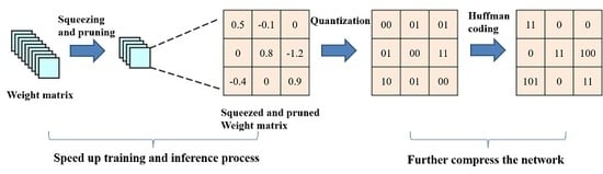
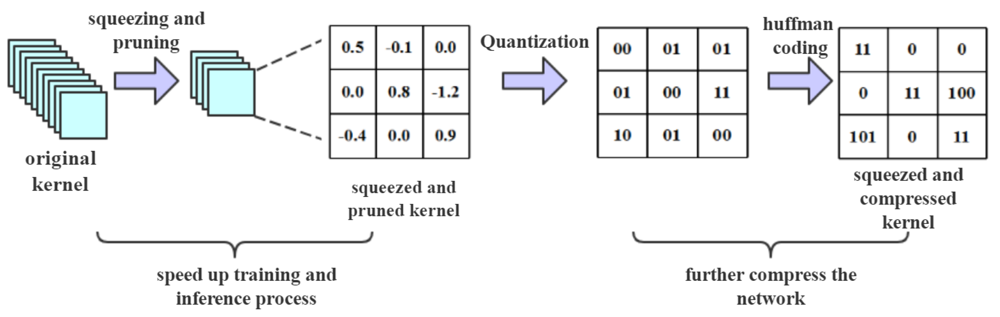
• We design a resource-constrained environment oriented CNN for SAR ATR using the pruning, compression and the fast convolution computation to achieve a high compression ratio efficiently while maintaining the considerable accuracy. (The whole process is shown in Figure 1)

The rest of this paper is organized as follows. Section 2 explains the details of our compression method and fast algorithm. Then experimental statistics and analysis are presented in Section 3. Finally our conclusions are drawn in Section 4.

2. The Proposed Method

Recent research on CNN-based SAR ATR has focused on the accuracy improvement. Due to the deep neural network model and large amount of convolution calculations, it is difficult to deploy the ATR networks on mobile platform with limited hardware resources. The need for real-time target recognition will be hindered, thus limiting the ATR applications. However, the compression of deep neural networks is the most straightforward solution for the case. The network pruning method is a classical way to reduce the model size in that certain weights in each layer are too small to contribute to the feature transmission. Similarly, the cropping of convolution kernel, namely the squeezing method, will greatly reduce the number of model parameters. Moreover, the ATR problem is essentially a qualitative determination of the target category. In the sense, the representation of model does not have to be as high precision. After those structural level compression, the quantization and coding will be applied for further compression.

2.1. Quantified Microarchitecture Squeezing Method

We know that for a given accuracy level, there are multiple CNN architectures that can achieve that accuracy. However, the problem of identifying a slimmer CNN architecture is challenging. Recent works squeeze the architecture through a few basic guidelines or principles such as decreasing the number of input channels, but none of them quantify the squeezing ratio.

Here, we deploy the network pruning method to help us squeeze CNN architecture rather than trial and error. Network pruning is proved to be a efficient way to reduce the network complexity in early work [37]. All connections with weights below a threshold are removed from the network and neurons with zero input connections or zero output connections will also be pruned, as shown in Figure 2.

Based on network pruning, we define pruning ratio: $rati{o}_p$ and squeezing ratio: $rati{o}_s$ in each layer as follows:

$$rati{o}_p=\frac{thenumberofprunedweights}{thenumberoforiginalweights}$$

(1)

$$rati{o}_s=\frac{thenumberofsqueezedweights}{thenumberoforiginalweights}$$

(2)

We start training the network and then pruning the weight matrix in each layer without causing accuracy loss. According to the pruning ratio in each layer, we can measure the redundancy of each layer and squeeze those layers that have a large pruning ratio and redundancy. Because pruning only impacts the computation in one specific layer but squeezing will change the size of output and computation in the next layer, we should be careful when doing squeezing and choose a smaller squeezing ratio than the pruning ratio. Moreover, we do not squeeze the kernel size in small networks, e.g., squeezing a $3\times 3$ kernel to a $1\times 1$ kernel, since it is too aggressive and will cause great accuracy loss if only small-scale redundancies exist in the weight matrix. Instead, we reduce the number of channels in convolutional kernels or the number of hidden units in fully connected layers according to the squeezing ratio.

Finding the slim architecture could be an iterative process. Each iteration consists of a network retraining process followed by a network squeezing process. In first iteration, we can employ an aggressive squeezing strategy because the original network has the most significant redundancies. After first time iteration, the new and squeezed network needs to be retrained until it reaches the same accuracy level as the original network. If the accuracy of squeezed network drops a lot, we should reduce the squeezing ratio. Although the new network becomes much more sensitive to pruning and squeezing, we may do gentle pruning and squeezing to it. We will end the iterative process until the pruning ratio is small since it shows that the redundancy is small and keep squeezing the network is likely to hurt the performance.

Suppose we do iterative squeezing in a $5\times 5\times 32$ convolutional kernel. In first iteration, $60\%$ of weights in the kernel are pruned without accuracy loss, then we may squeeze it to a $5\times 5\times 16$ one. Here the pruning ratio is $60\%$ and the squeezing ratio is only $50\%$. In second iteration, we pruned $30\%$ of weights and squeeze $25\%$ of the kernel to a $5\times 5\times 12$. In third iteration, we can only prune $10\%$ of weights and will stop squeezing since the pruning ratio is too small. The process is shown in Figure 3.

2.2. Fast Algorithm for Pruned Network

After the pruning and squeezing process, we obtain a pruned network with a small pruning ratio. Like the example in Figure 3, the kernel will be squeezed untile the pruning ratio is small enough. In the end, the squeezed kernel has only $10\%$ weights pruned. So, the weight matrix in each convolutional layer of the network is not sparse enough to be stored in compressed sparse row (CSR) or compressed sparse columns (CSC) format. Here, we propose a new convolutional computation method to exploit the light-degree sparsity of pruned weights and activation input. Typically, a 2D-convolutional layer performs the computation as follows:

$$Z_{m,n}=ReLU(\sum _{i=1}^f\sum _{j=1}^f{w}_{i,j}{A}_{i+m,j+n}+b)$$

(3)

where $ReLU(·)$ (Rectified Linear Unit) indicates the commonly used activation function, w is the weight matrix with dimension $f\times f$, i represents the row number of w, j represents the column number of w, A is the input feature map, b is the bias, Z indicates the output feature map, m represents the row number of Z, n represents the column number of Z.

We perform the multiplication only for non-zero $w_{ij}$ and elements $A_{i+m,j+n}$. To fully exploit the sparsity of the activation input, we first store the non-zero values and indexes of each $A_{i+m,j+n}$ in dictionaries. It is a single-time cost computation and we do not need to pick out non-zero values $A_{i+m,j+n}$ in future computation any more. The detail of the computation approach is shown in Figure 4. Here, the size of kernel is $2\times 2$, so we partition the activation input into 4 groups and store the non-zero values in each group. Then, we calculate each non-zero weights, that is $w_{11}$ and $w_{22}$, and their corresponding non-zero input values. At last, we will add up the results of these two groups according to the index of each result. The results with same index in different group will be added together.

2.3. Weight Sharing and Quantization

Weight sharing is a common technique used to compress the network and reduce the number of bits needed to store for every weight. According to the weight sharing method discussed in Deep Compression, we adopt k-means weight sharing algorithm and take linear initialization between $[min,max]$ of the pruned weights, which helps to maintain the large weights. Then suppose that we can use k cluster indexes to represent n weights, we only need ${log}_2\left(k\right)$ bits to encode every cluster index.

Another thing we should notice is that our CPU does not allocate space in individual bits, but in bytes. Typically on a 32-bit processor, the compiler will allocate memory size as $S=4\times \frac{N+31}{32}$, where N is the bits sizes and S is the byte sizes. So we cannot store cluster indexes separately which will cause memory wasted, instead we should store all indexes together.The details of the algorithms is illustrated in Figure 5.

Commonly, we use 4 bytes to store each weight, then the compression ratio can be calculated as:

$$r=\frac{4\ast n}{4\ast \frac{(n{log}_2\left(k\right)+31)}{32}+4\ast k}$$

(4)

In Figure 5, we have a layer that has 4 input neurons and 4 output neurons, the weight is a $4\times 4$ matrix, some weights in the matrix are pruned to zero. In weight sharing, the weights are clustered to 4 bins (denoted with 4 colors), and all the weights in the same bin share the same cluster index and cluster center. Each cluster index is represented with 2 bits. The compression ratio is:

$$r=\frac{4\ast 16}{4\ast \frac{(16\ast {log}_2\left(4\right)+31)}{32}+4\ast 4}=2.68$$

(5)

2.4. Huffman Coding

The occurrence probability of each weight index is different, especially in the pruned layer. In pruned layers, the remained zero weights and weights with small absolute value can be easily clustered into one bin. Figure 6 shows the count of weight indexes in conv4 layer. It shows that large number of quantized weights are distributed around the mid-value, which is close to zero.

By adopting the Huffman coding which is an optimal prefix code used for lossless data compression, we can exploit the biased weights distributions and further compress the storage. More common weight indexes are represented with shorter coding and fewer bits. The experiment shows that the Huffman coding can save another $10\%$ of weights storage.

3. Experimental Result

3.1. Dataset and Image Preprocessing

We implement training, network squeezing, pruning, weights sharing and Huffman coding with Python and Tensorflow framework. Tensorflow is a multi-language neural network library and runs on various heterogeneous systems, ranging from mobile devices to distributed graphics processing unit (GPU) cluster. As to hardware environment, a work-station with two Intel Xeon E5-2683 CPUs and one NVIDIA Geforce GTX1080 Ti GPU is employed as the training and testing platform. The experiment data used in this paper were collected by the Defense Advanced Research Projects Agency (DARPA) and the Air Force Research Laboratory (AFRL) Moving and Stationary Target Acquisition and Recognition (MSTAR) program. In SAR ATR community, the MSTAR image data is almost the only public dataset for the ATR algorithms research and evaluation [6]. Hundreds of thousands of SAR images containing ground targets were collected, including different target types, aspect angles, depression angles, serial number, and articulation, and only a small subset of which are publicly available on the website [6]. The dataset consists of X-band SAR images with 1 foot by 1 foot resolution and 0∼360${}^{\circ }$ aspect coverage, which contains ten types of vehicle targets, as shown in Figure 7. Due to the appearance geometric similarity, complex backscattering and aspect sensitivity, it is difficult to discriminate a vehicle sample in a single image split. For example, T72, BMP2 and BTR70 are highly confusing in that they have similar appearance like gun barrel and crawler.

Generally, the SAR ATR algorithms will be evaluated in the Standard Operating Condition (SOC) and the Extended Operating Condition (EOC) [38]. The SOC experiment is defined as the set of testing conditions “very near” training conditions. The EOC experiments are defined to individually measure SAR ATR extensibility across EOCs: configuration, target versions, depression, number of classes, squint, aspect, serial number (SN) and so on. Different from the recognition performance oriented ATR, the deep neural networks compression-based ATR aims to reduce the computation and memory of network model while maintaining considerable recognition accuracy. Therefore, two experiments with different recognition requirements in SOC are designed to evaluate the compression performance, respectively, the 3-class and 10-class recognitions. For the 3-class SOC experiment, three kinds of vehicle targets (T72, BMP2, BTR70) are used to evaluate the effectiveness of compressed deep network design. As for the 10-class SOC experiment, all the ten types of vehicle targets are used to evaluate the applicability to complex multi-classification problem. To meet the requirement of SOC experiment, the image sets with same serial number and different depression angle are selected as the training and testing sets, as listed in

Table 1. Training and Testing Images for the SOC Experimental Setup.

		Train		Test
Class	Serial No.	Depression	Quantity	Depression	Quantity
T72	132	${17}^{\circ }$	232	${15}^{\circ }$	196
BMP2	9563	${17}^{\circ }$	233	${15}^{\circ }$	196
BTR70	C71	${17}^{\circ }$	233	${15}^{\circ }$	195
BRDM2	E71	${17}^{\circ }$	298	${15}^{\circ }$	274
ZIL131	E12	${17}^{\circ }$	299	${15}^{\circ }$	274
2S1	B01	${17}^{\circ }$	299	${15}^{\circ }$	274
BTR60	7532	${17}^{\circ }$	256	${15}^{\circ }$	195
D7	3015	${17}^{\circ }$	299	${15}^{\circ }$	274
T62	A51	${17}^{\circ }$	299	${15}^{\circ }$	196
ZSU23/4	D08	${17}^{\circ }$	299	${15}^{\circ }$	274

.

In our paper, we adopt central sampling since the target located in the center of the image contains most important information while peripheral region of the image contain little information. So we centrally sample several $88\times 88$ patches from the original image, which is illustrated in Figure 8. We find out this preprocessing will accelerate the training and reduce computation without accuracy loss.

3.2. Squeezed Network

Figure 9 shows architectures of the original network and squeezed network. The squeezed network has only $18\%$ parameters of the original network without accuracy loss. The squeezing method reduces the number of multiplication by $5.7\times$.

The two plots in Figure 10 show the training time of squeezed network and original network when they are implemented in CPU and GPU respectively. In each plot, both squeezed network and original network can achieve $98\%$ accuracy after enough training time. However, compared to original network, squeezed network can get to the same accuracy level with much shorter time. This time reduction is critical for real time image processing. The detailed comparison of training time and inference time are drawn in

Table 2. Training time of squeezed network and original network in CPU and GPU.

	CPU Training (min)		GPU Training (s)
Accuracy Level	Squeezed Network	Original Network	Squeezed Network	Original Network
80% accuracy	4.3	10.6	3.3	4.5
90% accuracy	7.5	33.5	4.4	11.2
95% accuracy	14.1	72.2	7.4	17.6
98% accuracy	41.7	165.6	19.2	36.8

and

Table 3. Single sample inference time with squeezed network and original network in CPU and GPU.

	CPU Training (s)		GPU Training (ms)
	Squeezed Network	Original Network	Squeezed Network	Original Network
Time cost	0.24	1.16	2.09	4.83

. In training and inference process, the squeezed network is $4\times$ and $2\times$ faster than original network in CPU and GPU respectively. The inference process of compressed network is 2–4 times faster than the original network. This means the compressed network can calculate the result label for a image much faster and achieve the realtime response. Moreover, we can even retrain a newer and more suitable network with new image data in a specific problem rather than using the unchanged original network, as the retraining process costs only a few seconds.

3.3. Speed Up of Fast Algorithm in Pruned Convolutional Layers

During iterative squeezing, the network becomes more and more sensitive to squeezing and pruning. When we end up the squeezing process, we find out that only small-scale redundancies exist in conv3 and conv4 layers which have 80% parameters of the squeezed network. $84\%$ parameters and $78\%$ parameters can be pruned in conv3 and conv4 layers respectively without accuracy loss. Then the fast algorithm is adopted to fully exploit the sparsity of pruned weights and activation input, thus further reducing the number of multiplication by $3\times$ and $3.8\times$ in conv3 and conv4 layers. Combined with squeezing, we can reduce the number of multiplication by nearly $15\times$.

When applying our fast computation algorithm, we need to spend extra time creating dictionary to store non-zero value of activation input. Here, Figure 11 shows the time ratio of creating dictionary and multiplication in conv3 and conv4 layers. The ratio of creating dictionary is very small and often negligible. Besides, the computation speed up of our fast algorithm is showed in Figure 12. Fast algorithm gives another speed up by $2.9\times$ and $3.5\times$ in conv3 and conv4 layers.

3.4. Compression Result and Confusion Matrix

After squeezing and pruning the network, we do the experiments of weight sharing, quantization and Huffman coding. In weight sharing, we find 16 or 32 centroid are enough in each layer because our squeezed network only has 150 K parameters and pruning leaves many zero value in squeezed conv3 and conv4 layers. Figure 13 shows how accuracy drops with fewer bits per weight in each layer.

The details of our compression statistics are shown in

Table 4. Compression statistics in SOC 3-class experiment. S: squeezing, P: pruning, Q: quantization, H: huffman coding.

Layers	#Weights	Weights Size	#Weights (S + P)	Compress Rate (S + P)	Weights Bits (Q)	Weights Size (S + P + Q + H)	Compress Rate
Conv1	0.6 K	2 KB	0.3 K	$2.0\times$	4	0.2 KB	$10.0\times$
Conv2	40.8 K	159 KB	7.2 K	$5.7\times$	4	3.5 KB	$45.4\times$
Conv3	183.6 K	717 KB	24.2 K	$7.6\times$	5	17.6 KB	$40.7\times$
Conv4	691.2 K	2.63 MB	101.1 K	$6.8\times$	4	63 KB	$42.7\times$
Conv5	73.7 K	287 KB	15.5 K	$4.6\times$	5	9.5 KB	$30.2\times$
Fc1	13.8 K	54 KB	6.9 K	$2.0\times$	5	4.2 KB	$12.9\times$
Total	1 M	3.82 MB	155.2 K	$6.4\times$		98 KB	$39.9\times$

. Huffman coding can give an extra compression but the effect is small. The result shows that compressed network will be able to fit in an on-chip SRAM and have modest bandwidth requirement.

Table 5. 3-class recognition accuracy comparison of original network and compressed network.

Class	T72	BMP2	BTR70	Total
Original	0.978	0.986	0.985	0.983
Compressed	0.978	0.986	0.985	0.983
Difference	0.000	0.000	0.000	0.000

shows the confusion matrix of the original network and compressed network. Each row in the confusion matrix denotes the actual target class and each column represents the class predicted by two networks. The accuracies of original network and compressed network are both around $98\%$. Normally, the recognition performance will be degraded when the deep networks are simplified and compressed. The identical recognition results come from two aspects. First, the experiment is a relative simple 3-class recognition, the compressed networks may reach the accuracy as good as the original one. Second, it depends on our compression strategy, namely, maintaining the accuracy. We choose the proper compression rate to balance the accuracy and network size, and will stop keeping compress the networks before the accuracy drops. So our compression method does not harm the performance of neural network for SAR ATR.

We also test the compression effect in the same neural network model with MSTAR benchmark data set which contains ten different categories. The details of our compression statistics and accuracy comparison are shown in

Table 6. Compression statistics in 10-class recognition experiment. S: squeezing, P: pruning, Q: quantization, H: huffman coding.

Layers	#Weights	Weights Size	#Weights (S + P)	Compress Rate (S + P)	Weights Bits (Q)	Weights Size (S + P + Q + H)	Compress Rate (S + P + Q + H)
Conv1	0.6 K	2 KB	0.6 K	$1.0\times$	6	0.4 KB	$5.0\times$
Conv2	40.8 K	159 KB	28.8 K	$1.4\times$	5	17 KB	$9.3\times$
Conv3	183.6 K	717 KB	105.6 K	$1.7\times$	5	64 KB	$11.2\times$
Conv4	691.2 K	2.63 MB	457.6 K	$1.5\times$	5	279 KB	$9.6\times$
Conv5	73.7 K	287 KB	44.9 K	$1.6\times$	5	27 KB	$10.6\times$
Fc1	46 K	180 KB	34.5 K	$1.3\times$	6	25 KB	$7.2\times$
Total	1.035 M	3.94 MB	672 K	$1.5\times$		412 KB	$9.8\times$

and

Table 7. 10-class recognition accuracy comparison of original network and compressed network.

Class	2S1	BMP2	BRDM2	BTR70	BTR60	D7	T62	T72	ZIL131	ZSU23/4	Total
Original	0.901	0.912	0.843	0.969	0.923	0.974	0.904	0.923	0.916	0.948	0.915
Compressed	0.897	0.867	0.846	0.969	0.902	0.970	0.897	0.943	0.919	0.937	0.920
Difference	0.004	0.045	−0.003	0.00	0.021	0.004	0.007	−0.020	−0.003	0.011	0.005

. Although the 6-layer neural network is enough or even redundant for the 3-classification task discussed above and achieve $40\times$ compression rate, this model is relatively too shallow to get a high original accuracy and compression rate. Overall, we can only get a $10\times$ compression rate and the accuracy of compressed network is only $91.5\%$, which is $0.5\%$ lower than the original one. With a same neural network, when doing easy classification task, it will become relatively redundant and can be compressed more significantly. However, when the classification is complex such as the 10-classification task here, this network seems rather shallow and can’t even get a satisfying classification accuracy, not to mention compressing this slim network.

4. Conclusions and Future Work

Inspired by the recent compression and fast computation methods for deep neural network, we address the problem of usage of convolutional neural network for SAR-ATR in mobile applications such as unmanned aerial vehicle (UAV). Since the redundancy in our network is not very significant, we use pruning to quantify our squeezing ratio rather than trial and error to avoid great accuracy loss. Moreover, we provide a new idea of fast computation for pruned network which can reduce the number of multiplication by $3\times$ and save the training time by $3\times$. Finally, we combine squeezing, deep compression and our fast computation algorithm to compress the weight storage by $40\times$ and reduce the number of multiplication by $15\times$ without loss of accuracy. The compressed network still achieves $98\%$ accuracy of three-class classification but requires significant less memory storage and training time, which facilitate its usage in resource-constrained environment.

We plan to extend our work in the following directions. First, we expect that writing a CUDA code of our fast algorithm for pruned network and then comparing the training speed of our CUDA code with Caffe original network model and tensorflow original network model. Second, since the memory storage of our squeezed and deep compressed network is only 100 KB, we expect that we can store all the weights in register memory or shared memory in GPU which will speed up the I/O process. Finally, we expect that combining these two optimizations will reduce the training time even further.