Delineation of Built-Up Areas from Very High-Resolution Satellite Imagery Using Multi-Scale Textures and Spatial Dependence

Abstract

Very high spatial resolution (VHR) satellite images possess several advantages in terms of describing the details of ground targets. Extracting built-up areas from VHR images has received increasing attention in practical applications, such as land use planning, urbanization monitoring, geographic information database update. In this study, a novel method is proposed for built-up area detection and delineation on VHR satellite images, using multi-resolution space-frequency analysis, spatial dependence modelling and cross-scale feature fusion. First, the image is decomposed by multi-resolution wavelet transformation, and then the high-frequency information at different levels is employed to represent the multi-scale texture and structural characteristics of built-up areas. Subsequently, the local Getis-Ord statistic is introduced to model the spatial patterns of built-up area textures and structures by measuring the spatial dependence among frequency responses at different spatial positions. Finally, the saliency map of built-up areas is produced using a cross-scale feature fusion algorithm, followed by adaptive threshold segmentation to obtain the detection results. The experiments on ZY-3 and Quickbird datasets demonstrate the effectiveness and superiority of the proposed method through comparisons with existing algorithms.

1. Introduction

Built-up areas are important parts of a city, especially in urban areas. Rapid socio-economic development and increased population aggregation result in the spatial change of built-up areas through expansion, redevelopment and so on. The accurate detection and mapping of built-up areas can provide useful geospatial information for many applications [1], such as urbanization monitoring [2], disaster assessment [3], population estimation and mapping [4,5,6], and GIS database update [7]. Due to the increasing availability of remote sensing data, detecting and mapping built-up areas using satellite images is a very economical and efficient method.

Traditionally, built-up/urban areas are usually detected using medium- and coarse-resolution images (TM/ETM+, MODIS and DMSP/OLS, etc.) for large-scale applications [8,9,10,11,12,13,14]. With the rapid development of imaging techniques, satellite sensors can now provide images with a very high spatial resolution (up to submeter); therefore, built-up areas can be observed at a finer scale. In recent years, automatic detection of built-up areas from high-resolution satellite images has been a major area of interest [15,16]. However, higher spatial resolution does not mean higher detection accuracy because textures and structural patterns of built-up areas in the VHR images are more complex than those in median-low spatial resolution remote sensing images. Therefore, existing methods based on spectral information only for medium- and coarse-resolution images do not provide satisfying detection results when dealing with VHR remote sensing images.

To overcome these difficulties, many methods have been proposed to model the spatial patterns of built-up areas. Depending on whether or not the training samples are used, these methods can be divided into two categories: Supervised approaches and unsupervised approaches. The supervised approaches benefit from employing prior information of object samples, which can be used to train a classifier to achieve the discrimination between built-up and non-built-up areas. For instance, Li et al. [17] used multikernel learning to incorporate multiple features in the block-level built-up detection. More recently, convolutional neural networks (CNNs) were employed for the detection of informal settlements from VHR Images [18]. Built-up area extraction in temporary settlements was studied, and the proposed method was embedded in the methodological framework of object-based image analysis [19]. The performance of supervised approaches depends largely on the selected raining samples, and the construction of sample sets is time-consuming and laborious, especially for CNN models, which usually need large sample data so that their parameters can be well fitted. The unsupervised approaches, however, can avoid these weaknesses due to the fact that they do not need training samples in classification; hence, more attention has been paid to them by researchers in recent years. In this study, we briefly divided them into two categories: Local feature-based approaches and texture-based approaches.

With the increase of spatial resolution, local features (e.g., points, lines) of buildings become clearer, enabling them to be available features for built-up area detection. Sirmacek and Ünsalan [20] first extracted local feature points using Gabor filters to represent the existence of built-up features, and then used spatial voting to measure the possibility of each pixel belonging to built-up areas. After this work, corner points, edges or straight lines were employed to better locate building features, and their spatial distributions were modeled by spatial voting, density or other similar algorithms [21,22,23,24,25,26,27]. However, using only local features such as corners or lines are not sufficient to discriminate between built-up and non-built-up areas in complex scenes, because these features can also be detected in non-built-up areas. On the other hand, the spatial voting is a global algorithm and the computing time will increase sharply when the number of feature points or lines is large [28]. More recently, You et al. [29] proposed an improved strategy for built-up area detection. In their work, the local feature points were optimized by a saliency index and the voting process was accelerated adopting a superpixel based method. However, it should be noted that this method is suitable for multi-spectral images as the RGB bands of a multi-spectral image are needed for superpixel segmentation.

Texture-based approaches were proposed due to the fact that built-up areas have distinctive texture and structural patterns from the backgrounds in VHR images. A built-up presence index (PanTex) [30] was put forward based on the calculation of texture measures of contrast using the gray-level co-occurrence matrix (GLCM), and the effectiveness was verified on panchromatic SPOT images. Afterward, this index has been used for mapping global human settlements [31,32]. Nevertheless, the PanTex index is appropriate for satellite images with a resolution of about 5m, rather than a higher resolution. In a different work, Huang and Zhang [33] proposed a morphological building index (MBI) for automatic building detection, based on several implicit features of buildings (e.g., brightness, contrast, directionality and size). Later, the MBI algorithm was further developed to alleviate the amount of false alarms [34]. However, the performance of MBI and its improved algorithms are limited by the basic assumption that there is a high local contrast between buildings and their adjacent shadows, which is not always true. Also, they benefit from using multi-spectral information, and for single-band or panchromatic images, they may show degraded performance or even be inapplicable.

Considering the complexity of texture representation in the spatial domain, some frequency domain analysis methods were used to model the textural characteristics of built-up areas in recent years. Gong et al. [35] employed the Gabor filter to extract textural features for residential areas segmentation in Beijing-1 high-resolution (4 m) panchromatic images. Inspired by visual attention, a built-up areas saliency index (BASI) [36] was proposed to construct saliency map, which utilizes NSCT (nonsampled contourlet transform) to extract the textural features for saliency calculation of built-up areas. In the work of Zhang et al. [37,38], the quaternion Fourier transform and the lifting wavelet transform were introduced to describe the saliency for residential area or region of interest extraction in high-resolution remote sensing images. In summary, although these frequency domain- based methods were proven effective in extracting built-up areas by using multi-scale and multi-directional texture information, they pay more attention to the texture intensity in frequency domain than to their spatial distribution. As a result, local low-frequency areas in the interior of a built-up area are often missed while some high-frequency objects (e.g., roads) in the background are likely to be wrongly labeled as built-up areas. Apart from the texture intensity, taking advantage of the spatial contextual information may be a feasible strategy to solve this problem, due to the fact that spatial context, especially spatial dependence, is widely existing among pixels, features or objects in the image, and it has been proved to be very useful in improving the classification of objects [39,40,41]. In addition, an important fact that needs to be emphasized is that textures of built-up areas and their spatial dependence may show different characteristics and patterns under different spatial resolutions. The effective features for built-up areas discrimination may exist at different scales.

To effectively address this issue, we proposed a novel method for detecting and delineating built-up areas from VHR images by using multi-scale textures and spatial dependence. More specifically, the multi-resolution wavelet transform was employed for texture and structural feature representation of built-up areas at multi-scales. Furthermore, the local spatial Getis-Ord statistic [42,43] was introduced to model the spatial context patterns of built-up area textures and structures by measuring the spatial dependence among frequency responses at different spatial positions. The major contributions of this paper are summarized as follows:

(1)

To describe the complex textures of built-up areas, a maximization operation was introduced to integrate the multi-directional high-frequency components produced by multi-resolution wavelet decomposition, and the optimal scale for texture feature representation was explored by experiments.

(2)

Using local Getis-Ord statistic, the spatial context pattern of built-up area textures was modeled by measuring the spatial dependence among frequency responses at different spatial positions, which can make a single pixel capture the macro patterns of objects. Therefore, it can increase the saliency of built-up areas while suppressing the saliency of other objects such as some linear features (e.g., roads, ridge lines).

(3)

A cross-scale feature fusion based on the principal component analysis (PCA) was proposed to construct the final built-up area saliency map, which can effectively fuse the multi-scale high-frequency textures and spatial dependence.

The remainder of this paper is organized as follows. The proposed approach is presented in Section 2. Section 3 shows the experimental results and comparisons. The discussion and conclusion are provided in Section 4 and Section 5, respectively.

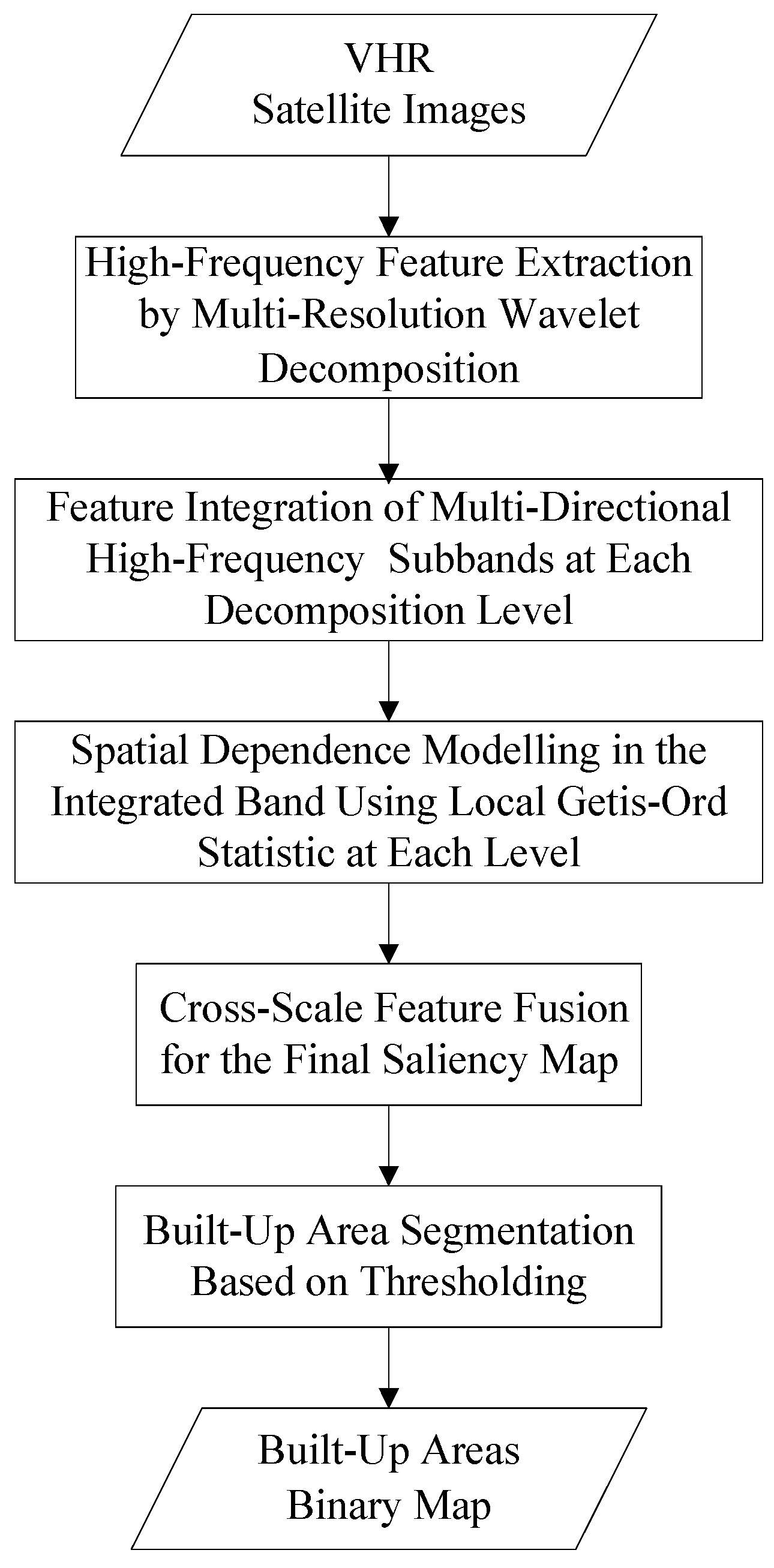
2. Proposed Method

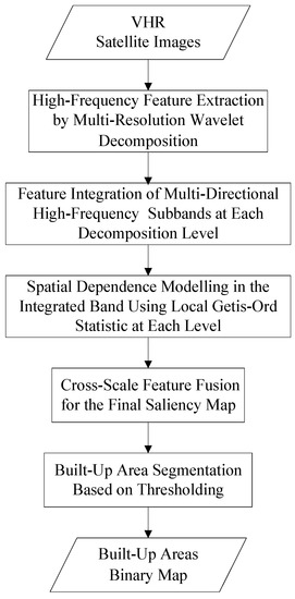
As shown in Figure 1, the proposed method is composed of five main steps: (1) multi-resolution wavelet decomposition and high-frequency feature extraction for the input image data; (2) feature integration of multi-directional high-frequency subbands by point-to-point maximization operation to produce a new feature band at each decomposition level; (3) spatial dependence modelling in the integrated band using local Getis-Ord statistic at each level; (4) cross-scale feature fusion using the principal component analysis (PCA) to construct the final saliency map; (5) built-up area segmentation based on thresholding.

2.1. High-Frequency Feature Extraction by Multi-Resolution Wavelet Decomposition

Compared with the Fourier transform and the window Fourier transform, the wavelet transform (WT) can automatically adapt to the requirement of the time (space) frequency signal analysis through the operation of dilation and translation, and focus on the details of signals at any scale. Mallat used the orthogonal wavelet basis to develop the multi-resolution analysis theory [44], which made the technology of wavelet analysis develop rapidly.

For the VHR image, it entails 2-dimensional signals, and the local space-frequency analysis can provide not only the frequency components but also their specific locations in the image, which would be very useful for the discrimination and positioning of built-up areas due to their distinctive textures and spatial patterns from the backgrounds. In this study, the multi-resolution wavelet theory was employed to derive the frequency information of built-up objects at different scales. Let f(x, y) denote a 2-dimensional gray image, and the multi-resolution wavelet decomposition can be expressed as follows [45].

$$\{\begin{array}{c}[A_{2^j},H_{2^j},V_{2^j},D_{2^j}]=WT(f)\\ [A_{2^{j+1}},H_{2^{j+1}},V_{2^{j+1}},D_{2^{j+1}}]=WT(A_{2^j})\end{array},$$

(1)

where $2^j$ (j ≥ 1) stands for the spatial resolution of the jth level of decomposition, and A is the low-frequency approximation component while H, V and D represent the high-frequency detail coefficients of three different directions (i.e., horizontal, vertical and diagonal, respectively). The Equation (1) can be calculated by the following convolution operations [46].

$$A_{2^j}f={(f(x,y)\ast {\varphi }_{2^j}(-x){\varphi }_{2^j}(-y)(2^{-j}n,2^{-j}m))}_{(n,m)\in Z^2},$$

(2)

$$H_{2^j}f={(f(x,y)\ast {\varphi }_{2^j}(-x){\psi }_{2^j}(-y)(2^{-j}n,2^{-j}m))}_{(n,m)\in Z^2},$$

(3)

$$V_{2^j}f={(f(x,y)\ast {\psi }_{2^j}(-x){\varphi }_{2^j}(-y)(2^{-j}n,2^{-j}m))}_{(n,m)\in Z^2},$$

(4)

$$D_{2^j}f={(f(x,y)\ast {\psi }_{2^j}(-x){\psi }_{2^j}(-y)(2^{-j}n,2^{-j}m))}_{(n,m)\in Z^2},$$

(5)

where m, n are integers; $\varphi (x)$ and $\psi (x)$ are one-dimensional scaling function (low-pass filter) and wavelet function (high-pass filter), respectively. The specific expression of the two functions depends on the selected wavelet types (e.g., Haar, Daubechies, etc.). For further details on wavelets properties and applications, you may refer to References [44,47]. In this study, the well-known Daubechies wavelets were selected for their superior performance in modeling the textural and structural patterns [45].

By implementing the multi-resolution wavelet decomposition, we can extract the high-frequency coefficients at multi-scales by neglecting the low-frequency approximation components. In our model, only the high-frequency coefficients, that is, $H_{2^j}$, $V_{2^j}$ and $D_{2^j}$ (j ≥ 1), are employed to model the texture characteristics of built-up areas, and more specifically, they are directly used as the feature maps representing the textural intensities in horizontal, vertical and diagonal directions, respectively.

2.2. Feature Integration of Multi-Directional High-Frequency Subbands

Assume L (L ≥ 1) levels of decomposition are performed and each high-frequency subband is used as a feature map, then 3 × L maps will be derived by this procedure due to the fact that each level of high-frequency coefficients includes three subbands (i.e., horizontal, vertical and diagonal, respectively). The multi-directional feature information is useful for built-up area discrimination, because the built-up textures and edges in the image usually have obvious directionality by human design and construction. To take advantage of multi-directional information, a point-to-point maximization operation was introduced for multi-directional feature integration, which can be formalized as follows.

$$I_{2^j}(x,y)=\max \{H_{2^j}(x,y),V_{2^j}(x,y),D_{2^j}(x,y)\},$$

(6)

where j = 1, 2, ···, L. Equation (6) was implemented for each decomposition level. By a maximization operation, the highest frequency detail coefficient will be selected, which can capture more effective features for built-up area discrimination. It should be noted that although this operator is simple, it is quite effective. Compared with some other operations such as average and absolute norm, the maximization operation can better capture the feature value characterizing the directionality of buildings, which is beneficial to enhancing the contrast between built-up and non-built-up areas in the subsequent saliency map.

2.3. Spatial Dependence Modelling Using Local Getis-Ord Statistic

The integrated high-frequency subband $I_{2^j}(x,y)$ (j = 1, 2, ···, L) describes the texture intensity at a spatial resolution of $2^j$ for the input original image, which can also be regarded as a texture saliency map from the perspective of computer vision. In practice, it is observed that the saliency values in certain locations of the built-up areas are still low, which is mainly caused by the lack or indistinctness of built-up features. Meanwhile, the high saliency can also occur in some background areas such as roads, which also have strong edge features.

Therefore, it is necessary to modulate the saliency maps in order to enhance the saliency in built-up areas while suppressing it in non-built-up areas. Ideally, it is expected that the saliency values in built-up areas are all higher than those of the backgrounds, which would be beneficial to built-up area segmentation by selecting an appropriate threshold. With this consideration, we proposed to use the local Getis-Ord statistic to model the spatial dependence among saliency values at different pixel positions in the texture saliency map. The Getis-Ord statistic was originally designed to measure spatial autocorrelation in geospatial data [42,43], and it is formally defined as

$$G_i{}^{*}(d)={\displaystyle {\sum }_{j=1}^n{w}_{ij}(d)}{x}_j/{\displaystyle {\sum }_{j=1}^n{x}_j},$$

(7)

where $G_i{}^{*}(d)$ is the Getis-Ord statistic for some distance d, $x_j$ is the attribute value at location j, and $\{w_{ij}(d)\}$ is a n × n spatial weight matrix, in which each value is a weight quantifying the spatial relationships between two locations [48,49] and n is the number of observations. The symmetric one/zero spatial weight is commonly used to define neighborhood relations. If the distance between location i and location j is less than the threshold parameter d, then $w_{ij}(d)=1$; otherwise, $w_{ij}(d)=0$. For a non-binary weight matrix, the value of $w_{ij}(d)$ usually varies with distance d, for example, it can be calculated according to a decay function of inverse distance.

In order to facilitate statistical inference and significance testing, Ord and Getis [43] developed a standardized version of $G_i{}^{*}(d)$ by taking the statistic minus its expectation, divided by the square root of its variance. The resulting measures are

$$G_i{}^{*}(d)=\frac{{\displaystyle {\sum }_{j=1}^n{w}_{ij}(d)x_j}-W_i{}^{*}\overline{X}}{s\sqrt{(n{\displaystyle {\sum }_{j=1}^n{w}_{ij}{(d)}^2-W_i{{}^{*}}^2)/(n-1)}}},$$

(8)

where $W_i{}^{*}={\displaystyle {\sum }_{j=1}^n{w}_{ij}(d)}$, $\overline{X}=\frac{{\displaystyle {\sum }_{j=1}^n{x}_j}}{n}$ and $s=\sqrt{\frac{{\displaystyle {\sum }_{j=1}^n{x}_j{}^2}}{n}-{(\overline{X})}^2}$.

In this study, the symmetric binary weights matrix is used. More specifically, we used an s × s (s = 2d + 1) neighborhood window to calculate $G_i{}^{*}(d)$ for each pixel i, and d is a pixel distance. If the pixel j is fall in the predefined window of the central pixel i, then $w_{ij}(d)=1$; otherwise, $w_{ij}(d)=0$.

The values of $G_i{}^{*}(d)$ measure the degree to which a pixel is surrounded by a group of similarly high or low values within a specified distance d. The advantage of the Getis-Ord statistic is its ability to identify two different types of spatial clusters, that is, high-value agglomeration (high-high correlation) and low-value agglomeration (low-low correlation), which are also called “hot spot” and “cold spot”, respectively. Significant positive values of $G_i{}^{*}(d)$ indicate a cluster of high attribute values while significant negative values of $G_i{}^{*}(d)$ indicate a cluster of low attribute values. The degree of spatial dependence or clustering and its statistical significance is usually evaluated by z-score and p-value. For example, if the z-score is greater than 1.65 or less than −1.65, it is at a significance level of 0.1 (90% significant), that is, the probability p (|z| > 1.65) = 0.1. Likewise, if |z| > 1.96, it is 95% significant (p = 0.05), and |z| > 2.58 is 99% significant (p = 0.01).

Using the Getis-Ord statistic, the saliency map can be modulated and the contrast between built-up and non-built-up areas can also be further enhanced, which would be beneficial to segment the built-up areas by a threshold-based algorithm.

2.4. Cross-Scale Feature Fusion to Construct the Final Saliency Map

Although the modulated saliency maps have been derived, each of them can only carry information of built-up areas at a single scale, based on which it is usually not enough to effectively differentiate between built-up areas and the background.

To take advantage of multi-scale texture and structural features for object discrimination, a principal component analysis (PCA) [50] based cross-scale feature fusion algorithm was proposed to construct the final saliency map. PCA is an orthogonal transformation, which can convert the original correlated variables into a new set of independent variables called principal components. By using the PCA procedure, the main information of the original variables is concentrated on the first few principal components.

Since the saliency maps derived above are at different scales, they cannot be directly used as the input of PCA. To perform the PCA procedure, the saliency maps at multi-scales are first interpolated to have the same size and resolution with the original image. Many interpolation algorithms can be used, such as the nearest neighbor interpolation, bi-linear interpolation and bi-cubic convolution interpolation. In our model, the bi-linear interpolation was used, which provides relatively good smoothness and relatively low computational cost. Subsequently, the principle component transformation was implemented and the first principal component was employed to construct the final saliency map.

2.5. Built-Up Area Segmentation through Thresholding

In the final saliency map, the built-up area as a whole usually has higher saliency values compared with its background. Therefore, a threshold can be selected to segment the built-up area from the background. To obtain the appropriate threshold, a trial and error approach may be used as in [16], but it is relatively time-consuming. The saliency map binarization is essentially a two classification problem. In this study, we adopt the well-known Otsu’s algorithm [51] to automatically select the optimal threshold for the binary built-up area detection map. The advantage of this algorithm is that it is a self-adaptive method to determine the threshold, based on the standard of maximum between-class variance which means the smallest error probability.

Furthermore, due to the use of Getis-Ord statistic for spatial dependence modeling, the two different types of spatial clusters, that is, high-value clusters (high-high correlation) and low-value clusters (low-low correlation), can easily be distinguished in the final saliency map, making the Otsu’s threshold appropriate to identify the built-up areas which usually correspond to the high-value clusters.

3. Experimental Analysis

To verify the validity of our proposed method, several experiments were conducted using a set of selected remote sensing images in different scenes and different spatial resolutions. The proposed method was compared with two previous approaches: The BASI algorithm [36] and Hu’s model [16] in order to further evaluate its overall performance. Three widely used metrics, that is, precision P, recall R, and F-measure were used to quantitatively evaluate the experimental results, which are defined as follows:

$$\mathrm{P}=\mathrm{TP}/\left(\mathrm{TP}+\mathrm{FP}\right),$$

(9)

$$\mathrm{R}=\mathrm{TP}/\left(\mathrm{TP}+\mathrm{FN}\right),$$

(10)

$$\mathrm{F}=2\mathrm{PR}/\left(\mathrm{P}+\mathrm{R}\right),$$

(11)

where TP, FP and FN stand for the number of true positive, false positive and false negative detected pixels, respectively. The F-measure (F) is a comprehensive index, which considers both the correctness and completeness and will be used to evaluate the overall performance of built-up area detection.

3.1. Dataset Description

In our experiment, two test datasets were collected from ZY-3 and Quickbird sensors, containing 22 satellite images and covering various geographic scenes. The main characteristics of ZY-3 and Quickbird sensors are shown in

Table 1. The main characteristics of ZY-3 and Quickbird satellites.

Satellite	Launch Date	Image Bands	Resolution
ZY-3	9 January 2012	Pan (nadir): 500–800 nm	2.1 m
		Pan (forward): 500–800 nm	3.5 m
		Pan (backward): 500–800 nm	3.5 m
		Blue: 450–520 nm Green: 520–590 nm Red: 630–690 nm Near IR: 770–890 nm	6 m
Quickbird	18 October 2001	Pan: 450–900 nm	0.6 m
		Blue: 450–520 nm Green: 520–600 nm Red: 630–690 nm Near IR: 760–900 nm	2.4 m

, and the two datasets used for performance evaluation are described in

Table 2. The dataset used for the detection of built-up areas.

Sensor	Image No.	Acquisition Site	Acquisition Date	Image Bands	Resolution
ZY-3	ZY3-1	Dengfeng City, China	3 February 2012	Panchromatic (nadir)	2.1 m
	ZY3-2
	ZY3-3
	ZY3-4
	ZY3-5
	ZY3-6
	ZY3-7
	ZY3-8	Lvliang City, China	23 August 2017
	ZY3-9
	ZY3-10
	ZY3-11
	ZY3-12
Quickbird	QB1	Wuhan City, China	16 July 2009	Pan-Sharpening Multispectral (Blue, Green, Red)	0.6 m
	QB2
	QB3
	QB4
	QB5
	QB6
	QB7	Dengfeng City, China	30 June 2011	Panchromatic
	QB8
	QB9
	QB10

.

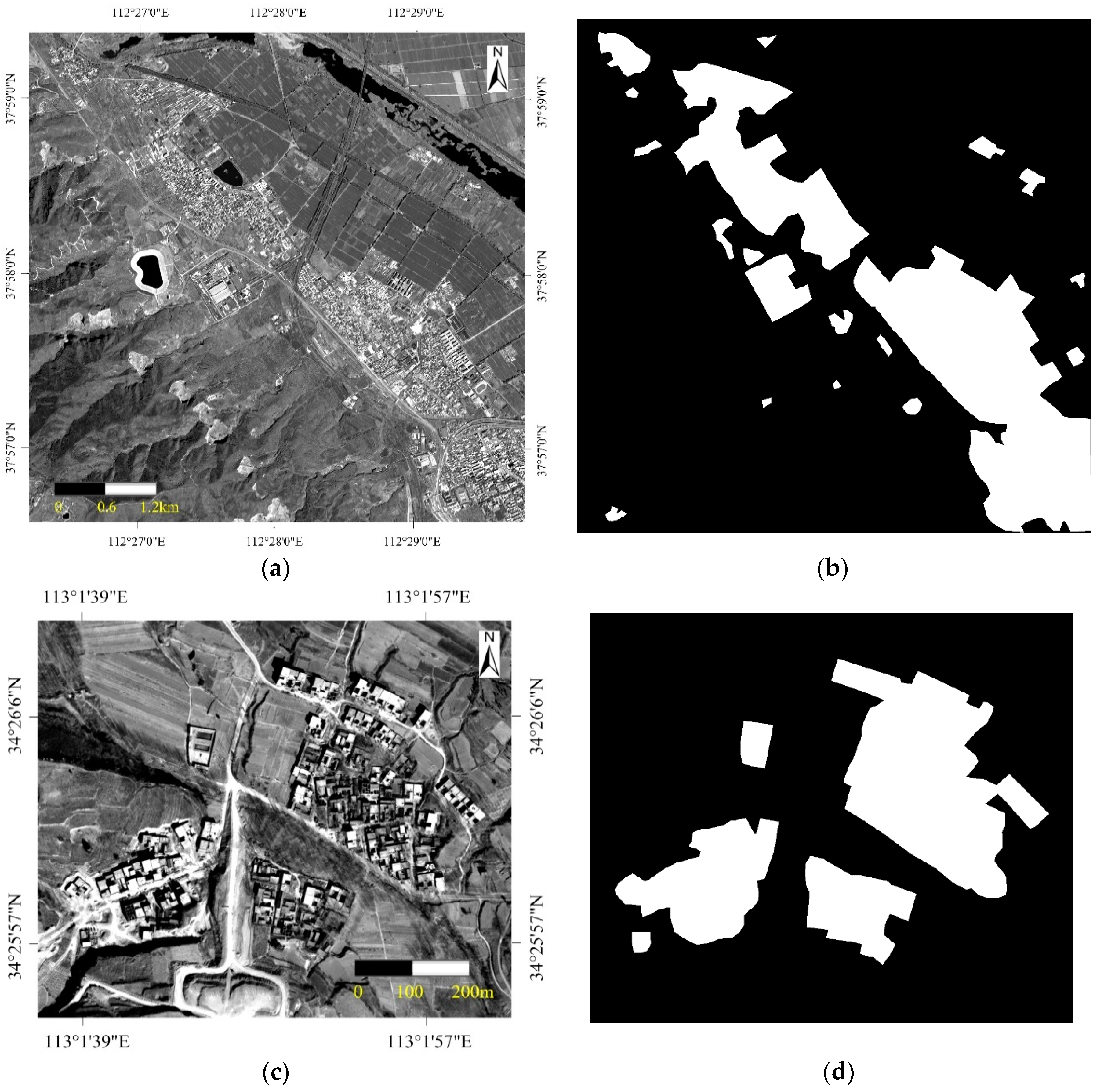
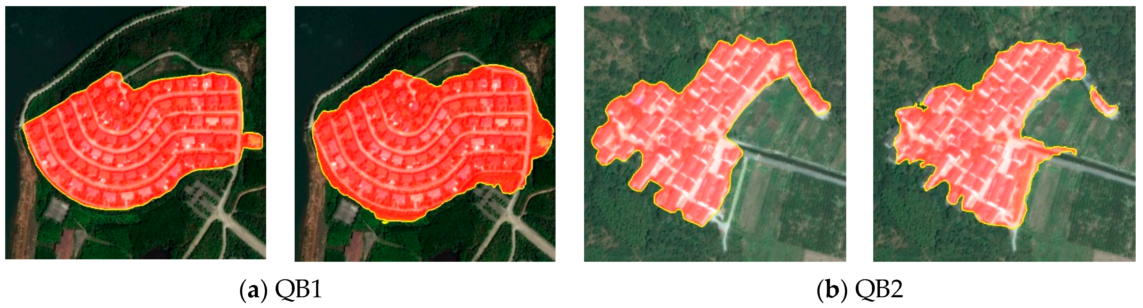
The first dataset is from the Chinese ZY-3 satellite, which is the first civil high-resolution stereo mapping satellite and was launched on 9 January 2012. The dataset contains 12 images, and all of them are taken from the nadir view panchromatic band with a resolution of 2.1 m. The images cover both flat and mountainous areas. One example image (i.e., ZY3-12) of this dataset is shown in Figure 2a, and Figure 2b is its reference image. The image, with a size of 2554 × 2557 pixels, contains several objects such as built-up areas, mountainous areas, farmlands, roads, rivers, etc.

The second dataset is from the Quickbird satellite, which is composed of 10 images, containing 6 pan-sharpening multispectral images and 4 panchromatic images. All of these images are with a resolution of 0.6 m. Figure 2c shows one example image (i.e., QB9) of this dataset, and its reference image is shown in Figure 2d. The test image (860 × 1016 pixels) covers a hilly area, and the built-up areas are of aggregated distribution in several neighboring positions. It is worth noting that for the multispectral images, we first convert the stacked RGB bands into gray images and then implement the proposed procedure, avoiding the effect of spectral confusion on built-up area detection.

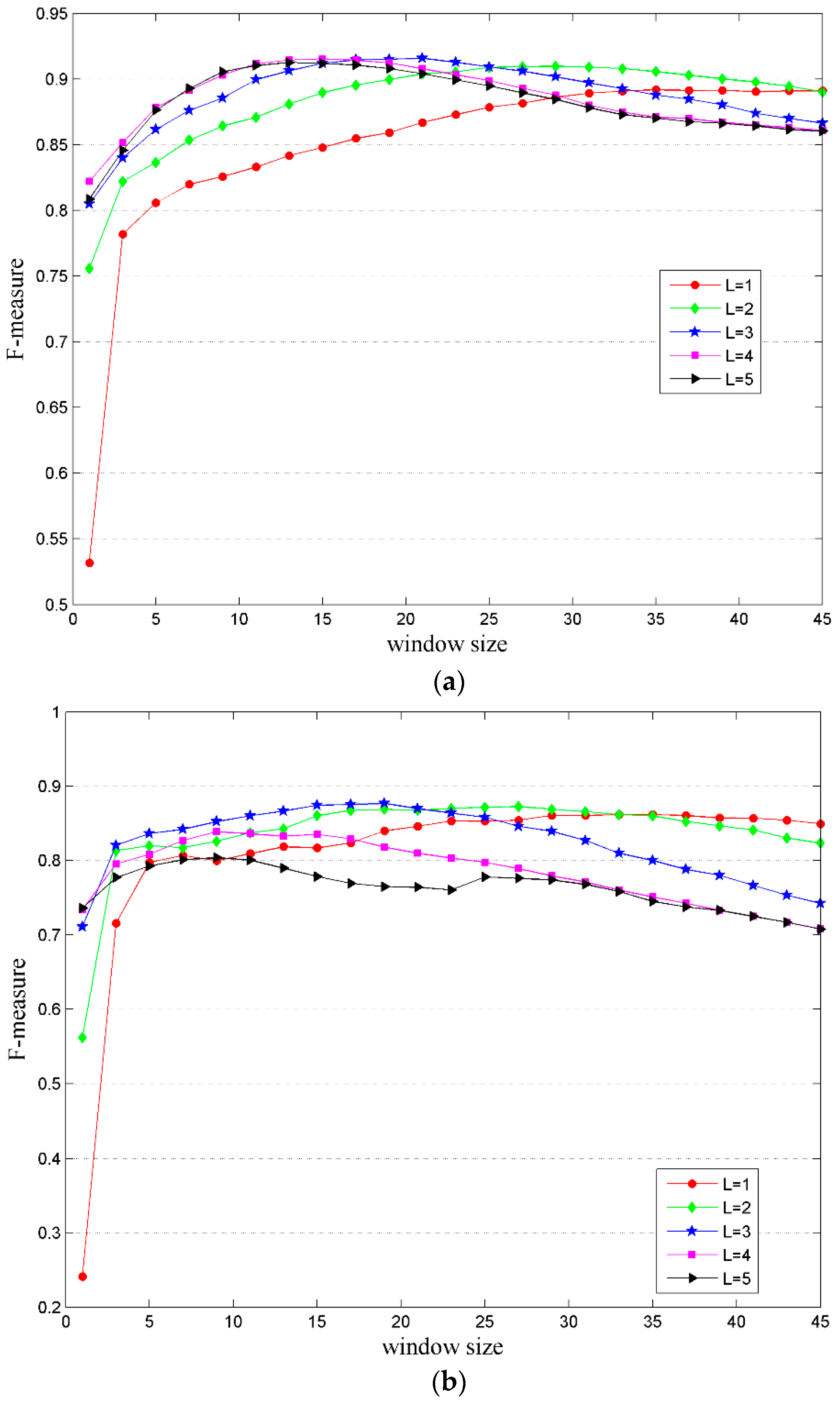
3.2. Parameter Tests

The main parameters of our model include the multi-resolution wavelet decomposition level L and the neighborhood window size s in the local spatial Getis-Ord statistic. Since each level of wavelet decomposition can obtain only detail information at the corresponding scale, the decomposition level L determines how many scales of high-frequency features will be used to construct the built-up area saliency map. Likewise, the window size s determines in what extents the local spatial dependence information is utilized to calculate the saliency for each pixel.

For parameter L and s, we conducted tests on the two example images shown in Figure 2. The quantitative evaluation based on the F-measure is presented in Figure 3, where each curve describes the change of F-measure as the window size s increases from 1 to 45 with step = 2 for L levels of wavelet decomposition, and five different values for L (i.e., L = 1, 2, 3, 4, 5) were tested, respectively; therefore, five curves were obtained for each example image.

As can be seen from Figure 3 that all curves have the following characteristics:

(1) With the increase of the window size, the overall performance of F-measure first increases and then decreases, but for different curves, the optimal window sizes (i.e., the maximum value point) are different. When the number of decomposition levels is less (e.g., L = 1, 2), a larger window size is needed to make F-measure obtain the maximum value. As the number of decomposition levels increases (e.g., L = 3, 4, 5), the maximum value point of the curve will move left, that is, only a smaller window size can meet the requirement.

(2) By comparing the corresponding curves of different decomposition level L, it can be found that when the size of the window is relatively small (e.g., s is less than 25), with the increase of L, F-measure also shows a trend of first increasing and then decreasing; therefore, the number of optimal decomposition levels exists for each fixed window parameter. For example, for the ZY-3 image in this case, when s = 20, the optimal decomposition level is L = 3, and when s = 30, the optimal decomposition level is L = 2.

Based on the above observations, we found that utilizing the multi-scale information by wavelet decomposition or using the local spatial dependence through the Getis-Ord statistic both can improve the accuracy of built-up area detection. To make the F-measure reach the maximum value (or approximate maximum value), a larger window size is needed when the number of decomposition levels is less and when the number of levels is large, a small window size can meet the requirement.

In term of the optimal values for parameter L and s, we think that they are data-dependent, that is, for different data, the optimal parameters are different. By testing different values for L on the two example images, we found that for the scale parameter, L = 3 is suitable for the aforementioned ZY-3 and Quickbird dataset, which can be tuned slightly according to the test images. In general, for the complex scene image, a relatively larger value of L is needed so as to better describe the difference between the built-up areas and their background.

Under this condition, the optimal window parameter s can be limited to a relatively small range in most cases. For the optimal value of s, the suggested search range is {3, 5, 7, 9, …, 29}, and the window size that makes the F-measure reach the peak is the optimal for s. The parameter combination (L, s) produced by this way may not be the optimal ones in some cases, but they can make the model reach the approximate optimal performance.

3.3. Results and Quantitative Evaluation

To evaluate the overall performance of our method, we conducted experiments for built-up area detection on the aforementioned ZY-3 and Quickbird datasets, respectively.

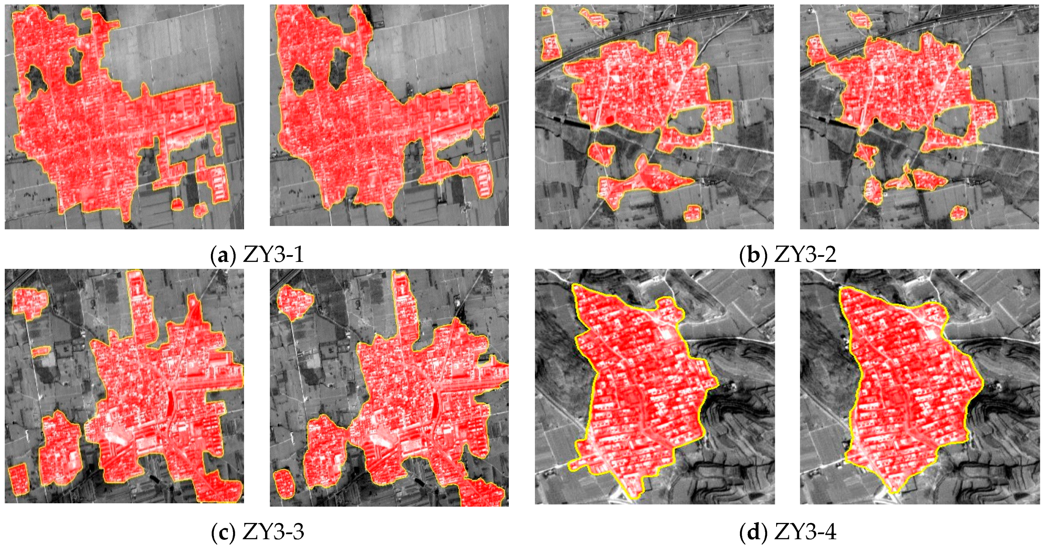
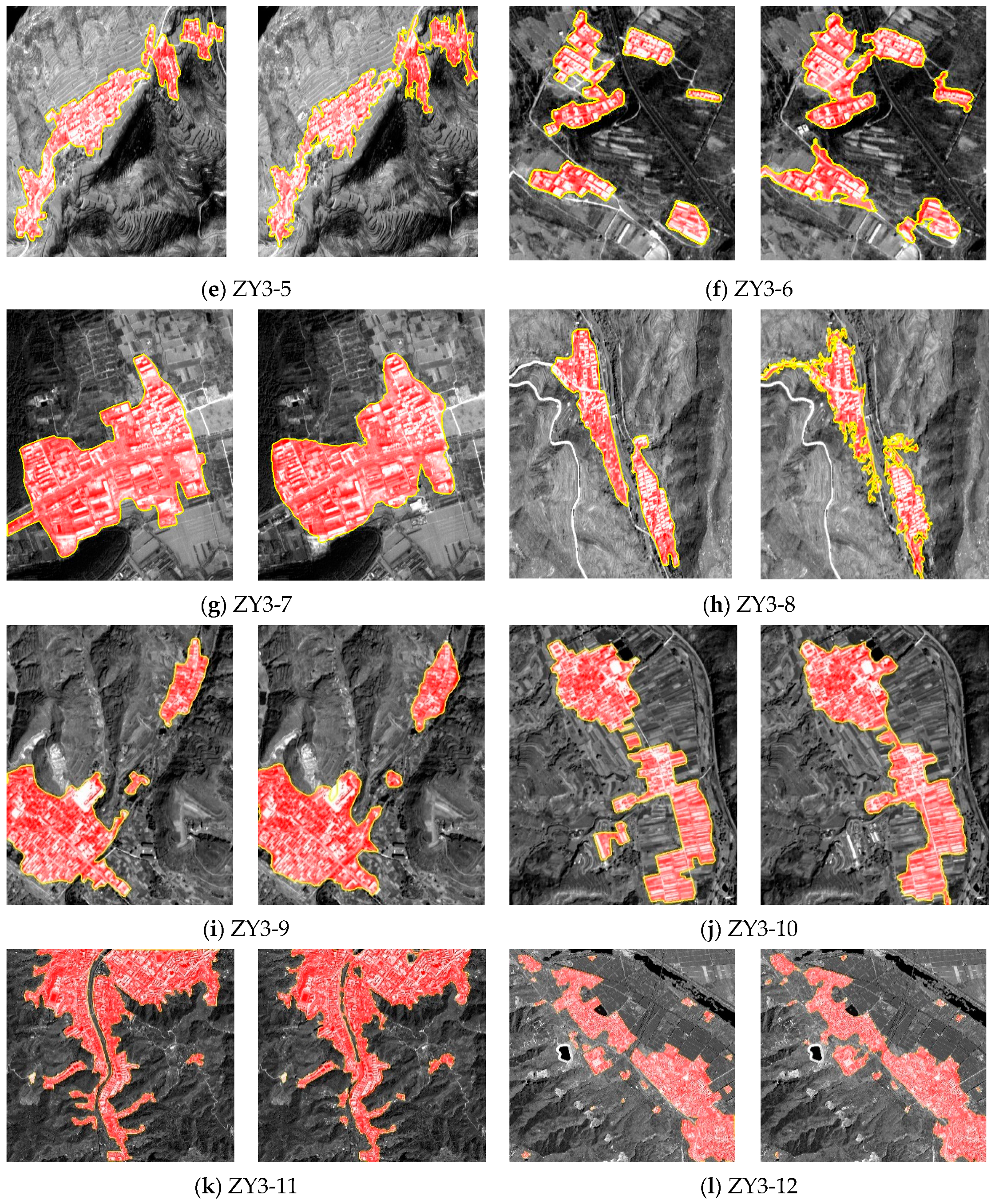
The detection results for the ZY-3 dataset are shown in Figure 4, where the first and third column are reference images while the second and fourth column are corresponding detection results, respectively. By visual comparisons, it can be found that each detection result is very close to its ground truth. The built-up areas in Figure 4a–c are located in a flat area, which can be easily detected with the proposed method, because the built-up areas have distinctive textures and structural features which would produce higher frequency responses than their relatively simple background. The images in Figure 4d–l cover several hilly and mountainous areas, and there are many valleys, ridges or trees in these areas, which have rich edges and textures. Like the built-up areas, they can also show high-frequency characteristics in the frequency domain. Despite the effects of these complex factors, the proposed method still performs well, and most of the built-up areas are identified successfully.

Table 3. Parameter settings and quantitative evaluation for the ZY-3 dataset.

Image No.	Parameter Settings		Statistics of the Performance
	L	s	P	R	F-Measure
ZY3-1	3	11	0.9603	0.9111	0.9351
ZY3-2	3	7	0.9497	0.8700	0.9081
ZY3-3	3	11	0.9687	0.9169	0.9421
ZY3-4	2	13	0.9711	0.9423	0.9565
ZY3-5	2	3	0.8185	0.8537	0.8357
ZY3-6	2	5	0.7007	0.9160	0.7940
ZY3-7	2	19	0.9057	0.8778	0.8915
ZY3-8	2	3	0.8208	0.7637	0.7912
ZY3-9	2	13	0.8715	0.9604	0.9138
ZY3-10	3	7	0.8790	0.8818	0.8804
ZY3-11	3	11	0.9199	0.9193	0.9196
ZY3-12	3	21	0.9202	0.9112	0.9157

reports the optimal parameters used and the result of quantitative evaluation for each of the dataset. As can be seen from the second column of this table, the optimal value for the scale parameter L is 3 or 2, which means that 2 or 3 levels of wavelet decomposition are suitable for the textural feature representation of built-up areas in ZY-3 images. The optimal window sizes show great differences for different images, ranging from 3 to 21. This may be caused by the difference between the spatial structures of different built-up areas. Take the built-up area in the image of ZY3-7 (Figure 4g) for example, there are multiple types of sub-objects with relatively homogeneous surfaces, which would produce relatively low frequency responses; therefore, a larger window size is necessary so as to obtain larger texture saliency values at these areas. With these parameter settings, overall, the proposed method achieved high F-measure values. For example, the F-measure value over the image of ZY3-4 (Figure 4d) is 0.9565 (P = 0.9711, R = 0.9423), which means that an approximate precise delineation of the built-up area boundary has been obtained. For the images of ZY3-6 (Figure 4f) and ZY3-8 (Figure 4h), the F-measure values are relatively low, which are 0.7940 and 0.7912, respectively. This may be caused by the complex hilly scenes, where the built-up areas are either scattered in the spatial distribution or small in the building size.

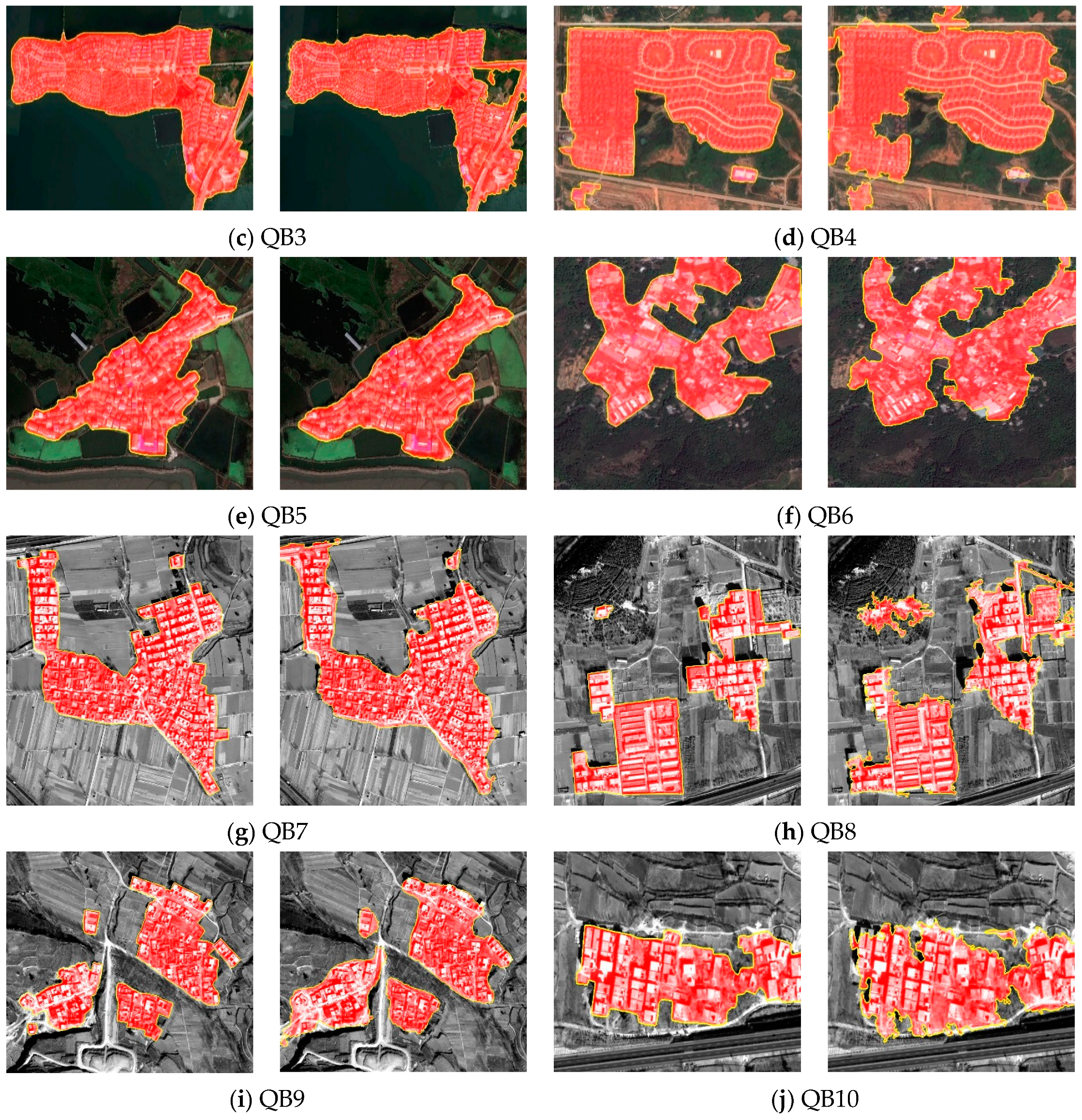
For the Quickbird dataset, the built-up area detection results are presented in Figure 5, where the pan-sharpened multispectral (Figure 5a–f) and panchromatic (Figure 5g–j) images were tested, respectively, which also cover both flat areas (Figure 5a–e) and hilly areas (Figure 5f–j). With the increase of spatial resolution, the built-up areas in these images show richer texture details and clearer geometric structures and spatial patterns. In this case, the texture representation based on a single pixel is unreliable, because the built-up areas show not only high-frequency characteristics in edge areas but also low-frequency responses in internal homogenous regions (e.g., roofs).

As shown in Figure 5, however, the proposed method is still applicable to Quickbird images, and show very good performance. The result of quantitative evaluation and the optimal parameters used for each of the dataset are listed in

Table 4. Parameter settings and quantitative evaluation for the Quickbird dataset.

Image No.	Parameter Settings		Statistics of the Performance
	L	s	P	R	F-Measure
QB1	3	25	0.8553	0.9978	0.9211
QB2	3	11	0.8890	0.8786	0.8838
QB3	2	5	0.9523	0.9458	0.9490
QB4	2	13	0.8919	0.9231	0.9073
QB5	3	11	0.9297	0.9682	0.9485
QB6	3	15	0.8574	0.9047	0.8804
QB7	3	15	0.9055	0.9598	0.9319
QB8	5	3	0.7392	0.8989	0.8112
QB9	3	19	0.8104	0.9552	0.8769
QB10	6	3	0.8141	0.9234	0.8654

. For all of the test images, the F-measure values are greater than 0.8. Although the spatial structures of built-up areas in these images are very complex due to the increased resolution, the built-up areas were detected successfully and their boundaries were well delineated. In addition, with regard to the scale parameter, L = 3 is still suitable for most of the test images. However, compared with the above ZY-3 dataset, the optimal values of the scale parameter L for texture and structural feature representation are slightly greater. Take the images of QB8 (Figure 5h) and QB10 (Figure 5j) for example, the optimal values of L are 5 and 6, respectively. This could be explained by the fact that the built-up areas in the two images are both more complex in textural patterns and spatial structures, and therefore, higher levels of wavelet decomposition are necessary so as to better model the spatial patterns of built-up areas.

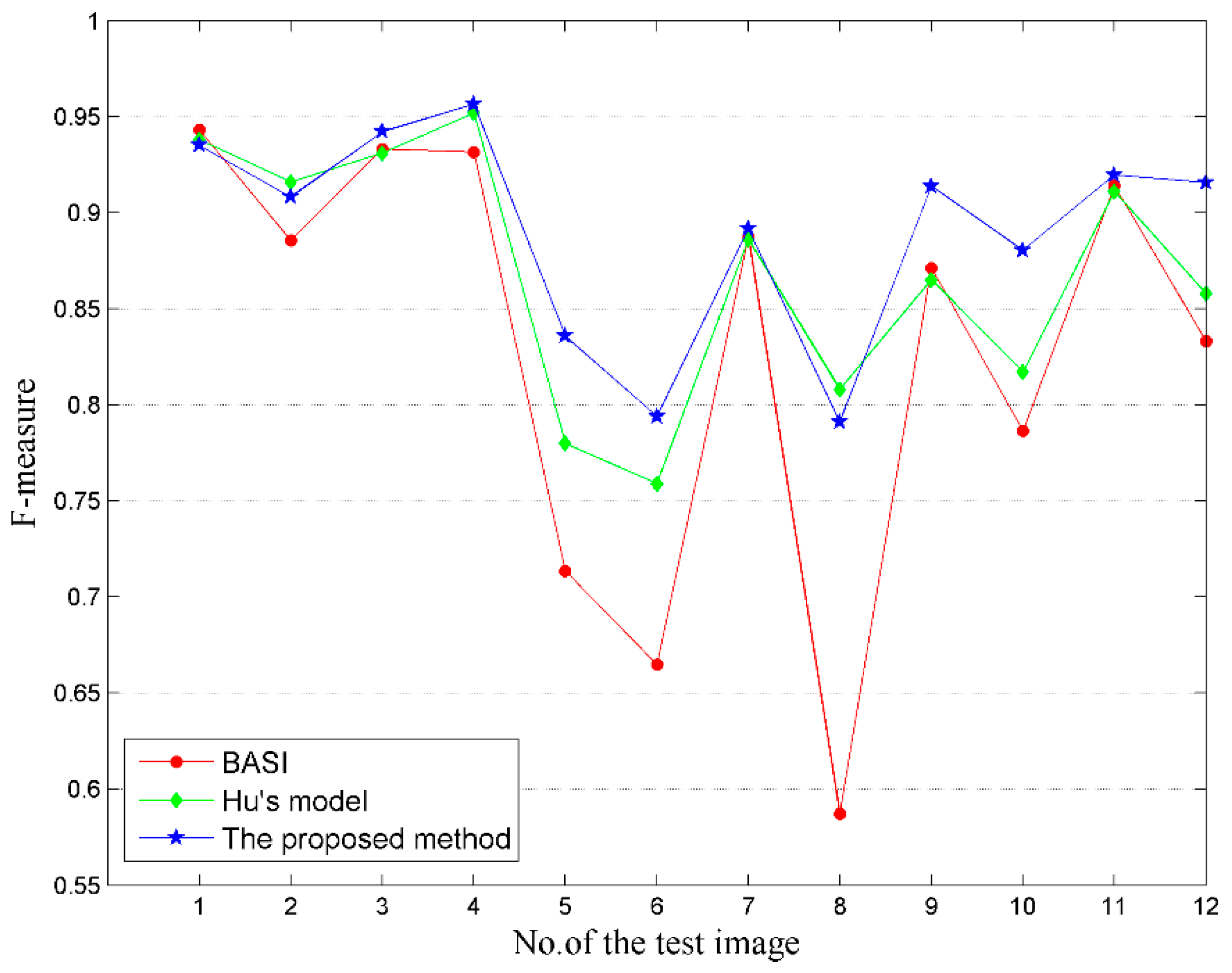
3.4. Comparisons with Other Algorithms

In this section, we compared our method with two similar approaches: The BASI and Hu’s model. The results of BASI were provided by the author of [36], and with the procedure provided by the author of [16], we obtained the optimal results of Hu’s model by adjusting the experimental parameters.

For the ZY-3 dataset, the accuracy comparisons are shown in Figure 6. As can be seen that the proposed method shows competitive performance over the two methods. For the images in flat areas (Figure 4a–c), all the three algorithms perform well (F > 0.85), but over hilly and mountainous areas, the proposed method, on the whole, shows better performance and the BASI algorithm shows greater fluctuations.

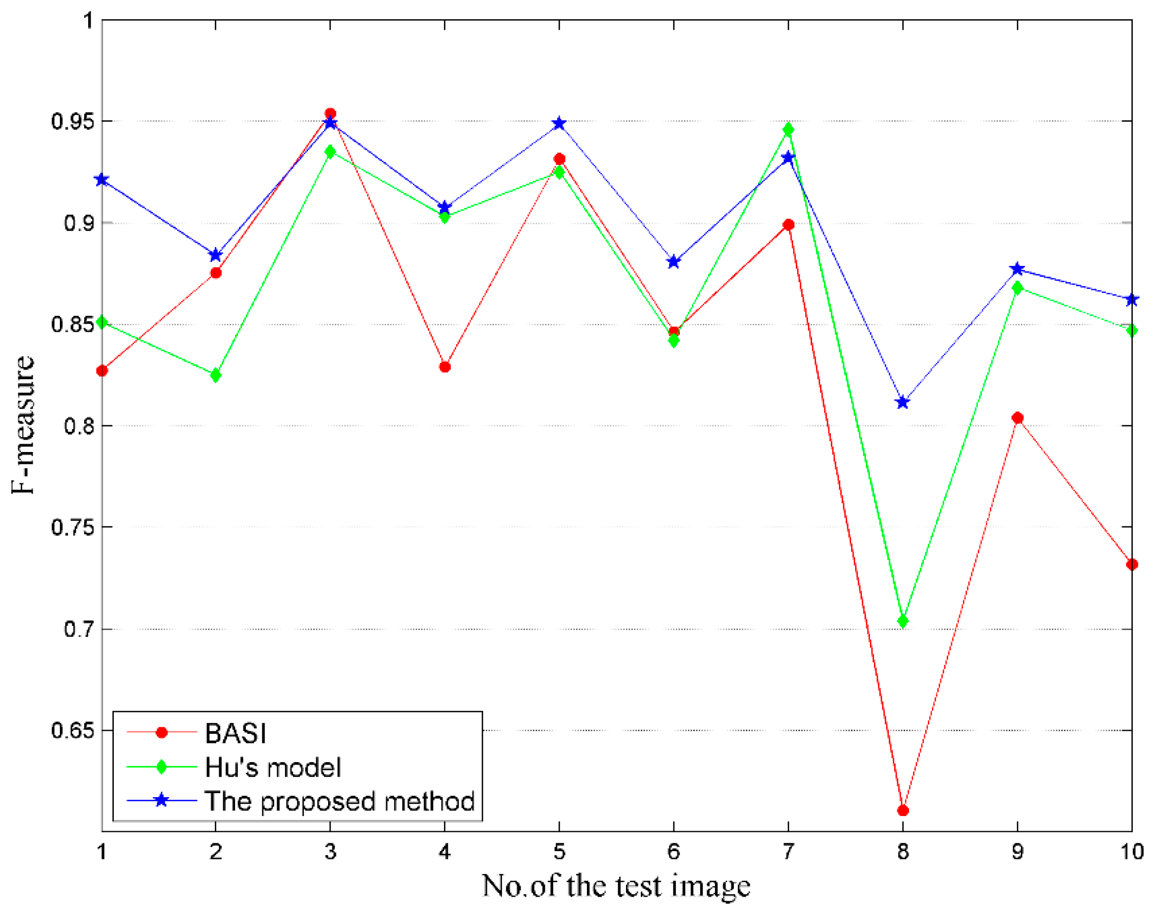
The accuracy comparisons for the Quickbird dataset are presented in Figure 7. On the whole, the proposed method also shows competitive performance, and it achieves higher F-measure values for almost all of the test images (apart from Figure 5c) than the BASI algorithm. The Hu’s model also performs well, but it shows greater fluctuations than the proposed method. For example, although the Hu’s model obtains a slightly higher F-measure value on the image of QB7 (Figure 5g) than the proposed method, it performs less effectively on the other images.

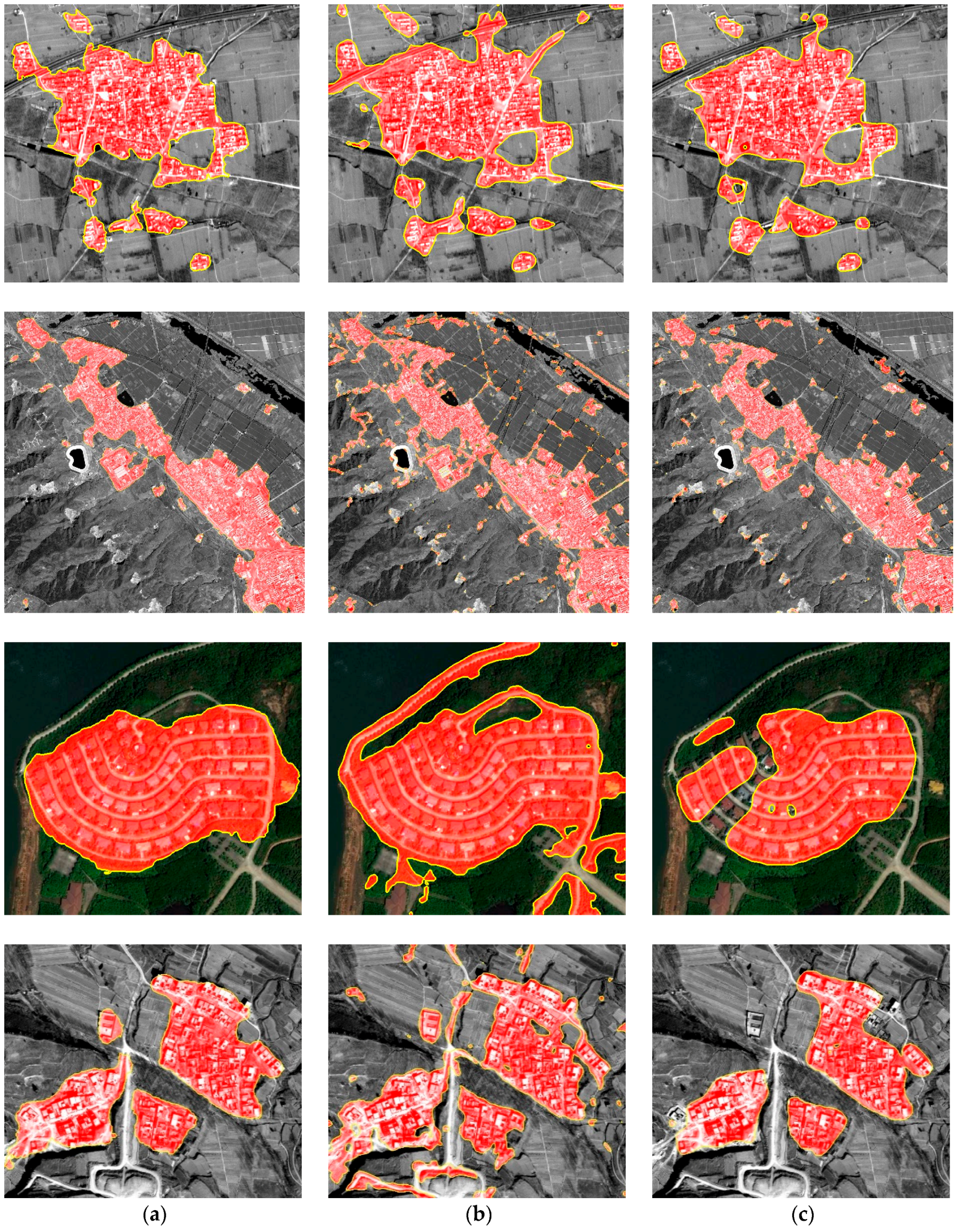
In order to visually compare the differences between the detection results using different methods, we list some typical examples of the detection results in Figure 8. It can be found that the results of the BASI algorithm are sensitive to some linear features such as roads, which often lead to false detection. Hu’s model avoids this weakness, but it can also lead to false detection (e.g., ZY-3 images in Figure 8) or missed detection (e.g., Quickbird images in Figure 8). In comparison to the two methods, the proposed method obtains relatively better results. In particular, it can effectively suppress some linear features (e.g., roads) in the background. The reason for such a result is that the contextual information of a pixel can be employed by measuring the spatial dependence based on the Getis-Ord statistic, and the macro-patterns, which are different between built-up areas and other linear features, can be obtained for this pixel.

4. Discussion

The above experimental results and performance comparisons indicate that the proposed method is more effective in built-up area detection for ZY-3 and Quickbird images, and overall, it shows a better performance than the BASI algorithm and Hu’s model.

The main parameters that should be set include the number L of multi-resolution decomposition levels and the window size s in the local spatial Getis-Ord statistic. We have given tests on how the two parameters affect the detection results based on the F-measure values and the parameters selection method is also provided.

Apart from the two parameters, there is, in fact, another important parameter: The threshold T, which is used to convert the saliency map into a binary detection result. In the proposed method, we use the well-known Otsu’s algorithm to automatically select the segmentation threshold, which is a unique value produced by the standard of maximum between-class variance for each test image. As a result, we did not do a further test on this parameter in the section of experiments. Using the Otsu’s algorithm, although we obtained good experimental results on the test dataset, the optimal thresholds produced do not necessarily lead to the optimal segmentation results for some of the images, which is a shortcoming of the proposed method.

Since the saliency map is constructed by measuring the local spatial dependence using the Getis-Ord statistic, with significant positive values indicating high-value clustering while significant negative values indicating low-value clustering. Therefore, the z-score and p-value could be used to evaluate the degree of spatial dependence for high-value clusters which usually correspond to the built-up areas. Taking this standard into consideration, the threshold can be further optimized so as to better improve the result of built-up area detection.

5. Conclusions

This study proposed a novel unsupervised method for built-up area detection in VHR satellite images. The texture and spatial patterns are represented by multi-resolution space-frequency analysis and spatial dependence modeling. A cross-scale feature fusion algorithm is proposed to construct the final built-up area saliency map, followed by thresholding to obtain the detection results. The experiments on both ZY-3 and Quickbird datasets demonstrate the effectiveness and superiority of the proposed method. It can be concluded that the effective features for built-up discrimination exist at multi-scales; therefore, the multi-scale representation of textures and structural features is a good and effective strategy for built-up areas detection. By fusing the spatial dependence into the multi-scale feature representation, the better detection results with well-defined shapes and boundaries can be obtained, and some linear features (e.g., roads, ridge lines) in the background can be effectively removed.

There are still several aspects that we can make to improve on the current work. For example, the degree of spatial dependence and its statistical significance can be evaluated by z-score and p-value, hence they could be used to further optimize the Otsu’s threshold so as to better improve the result of built-up area detection. Also, the image covering a larger area (e.g., urban or regional scale) may be tested to evaluate the potential of the proposed method in large-scale built-up area mapping with a finer spatial resolution.