Pléiades Tri-Stereo Data for Glacier Investigations—Examples from the European Alps and the Khumbu Himal


Abstract
:
1. Introduction
2. Materials and Methods
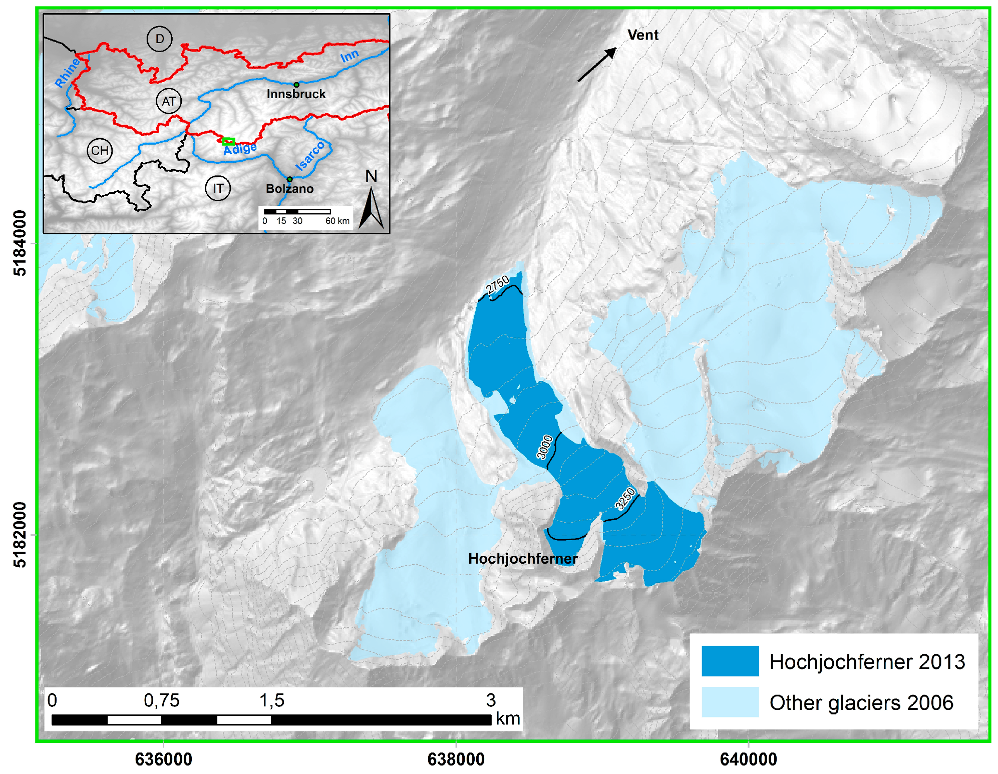
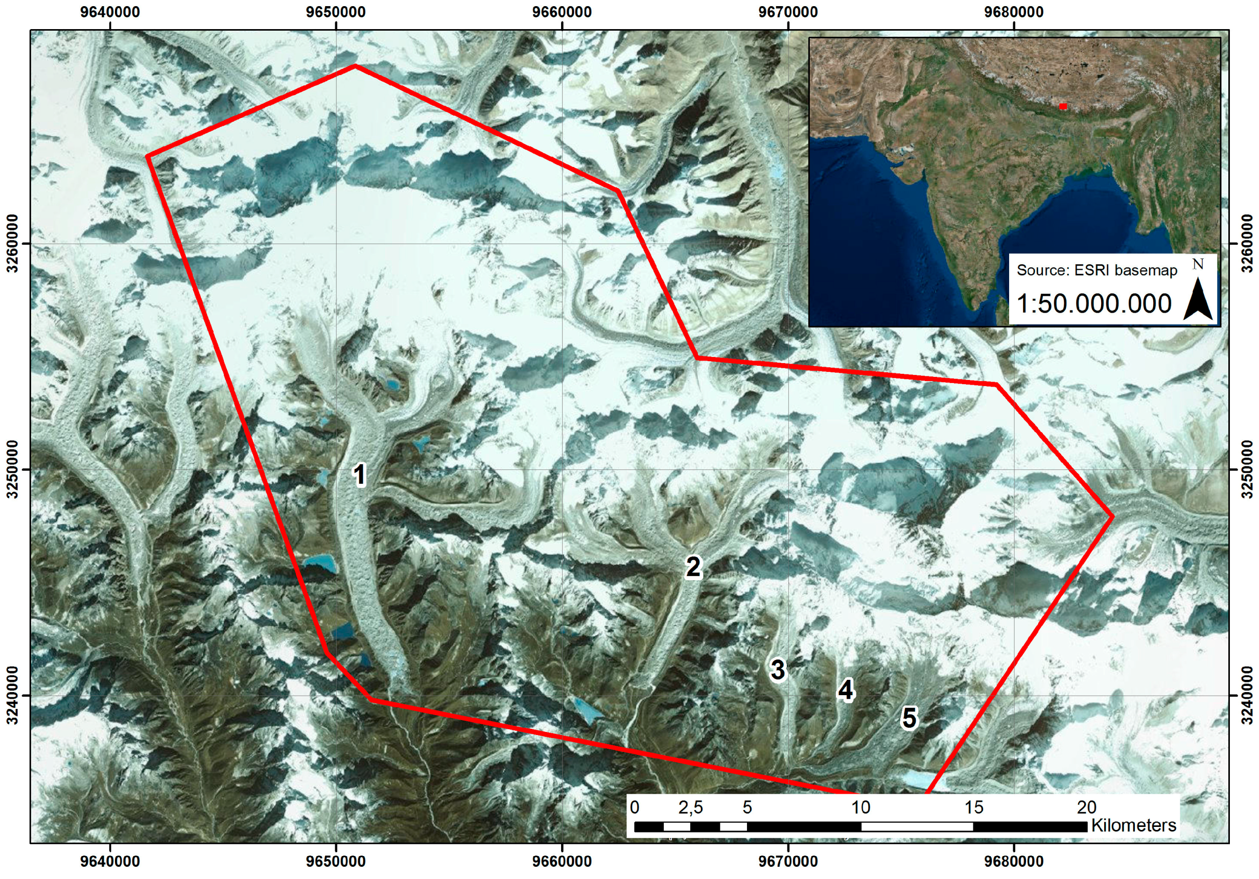
2.1. Study Areas
2.2. Data and Processing
2.2.1. Pléiades Data and Processing
2.2.2. ALS Data and Processing
2.2.3. Co-Registration
2.2.4. Analysis of Glacier Processes
3. Results I: DEM Quality
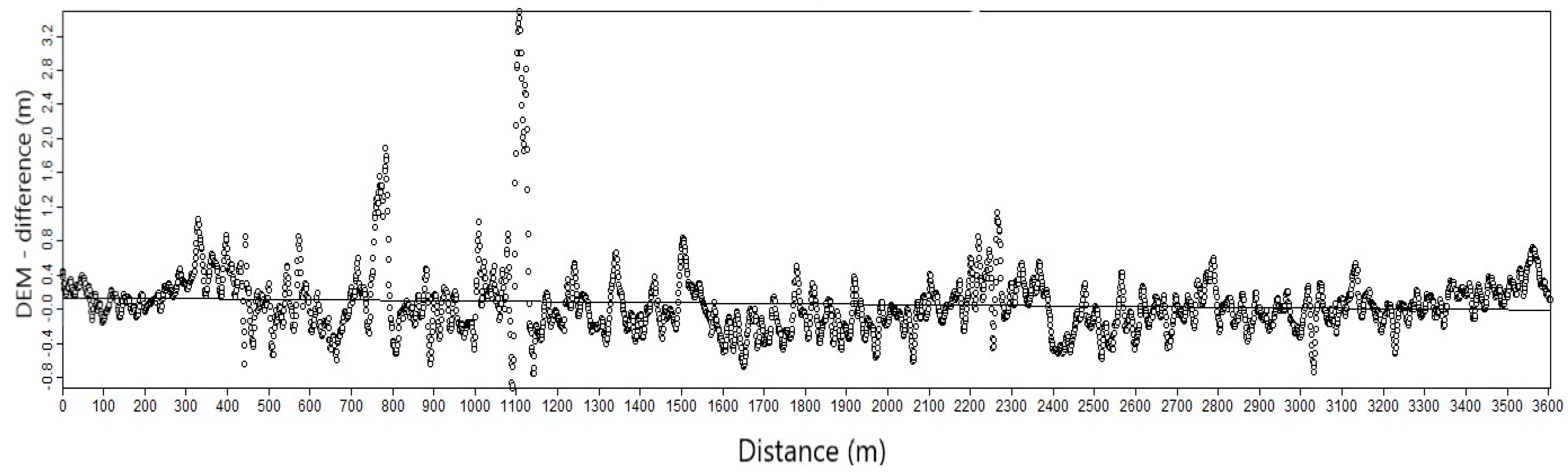
3.1. Comparison of Pléiades DEM with ALS-DEM in the European Alps
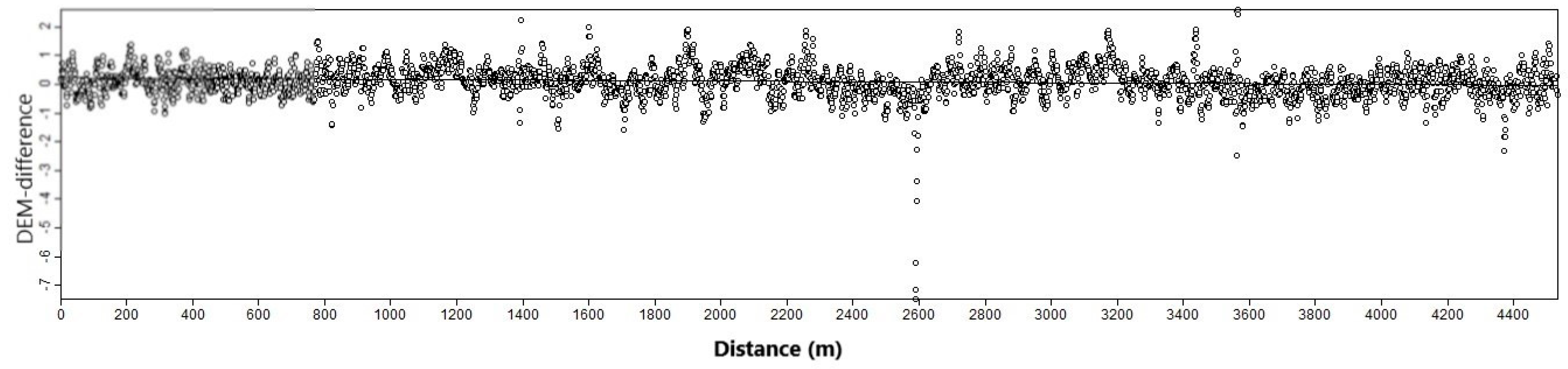
3.2. Accuracy of Khumbu Himal Pléiades DEM based on RPC
4. Results II: Glaciological Interpretation
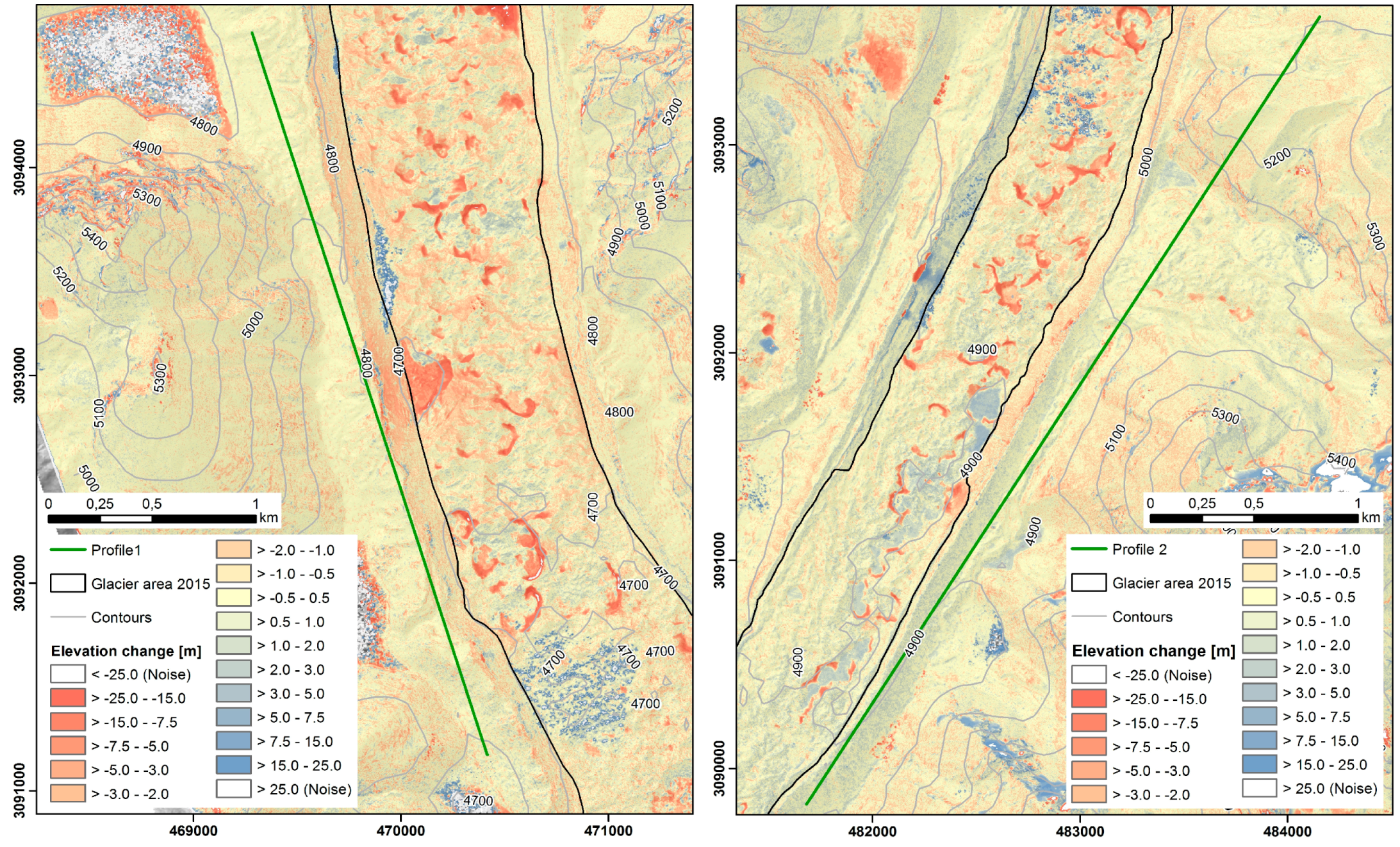
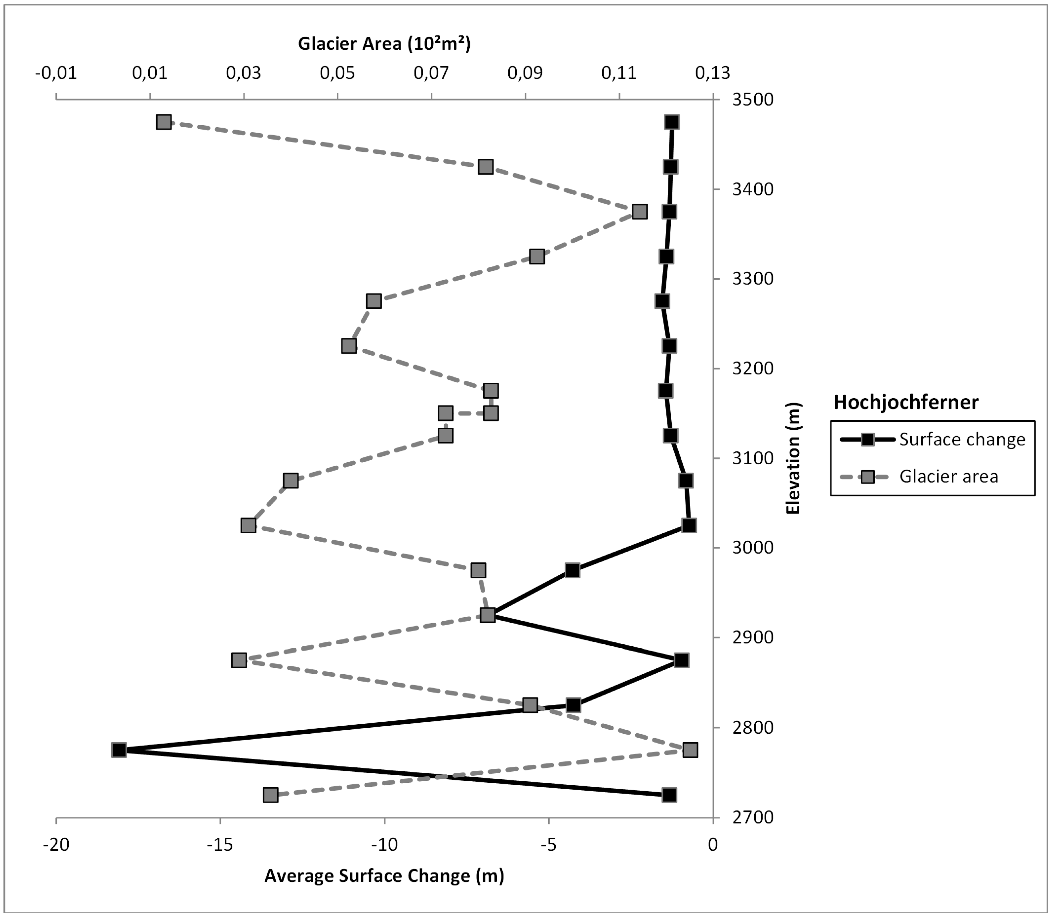
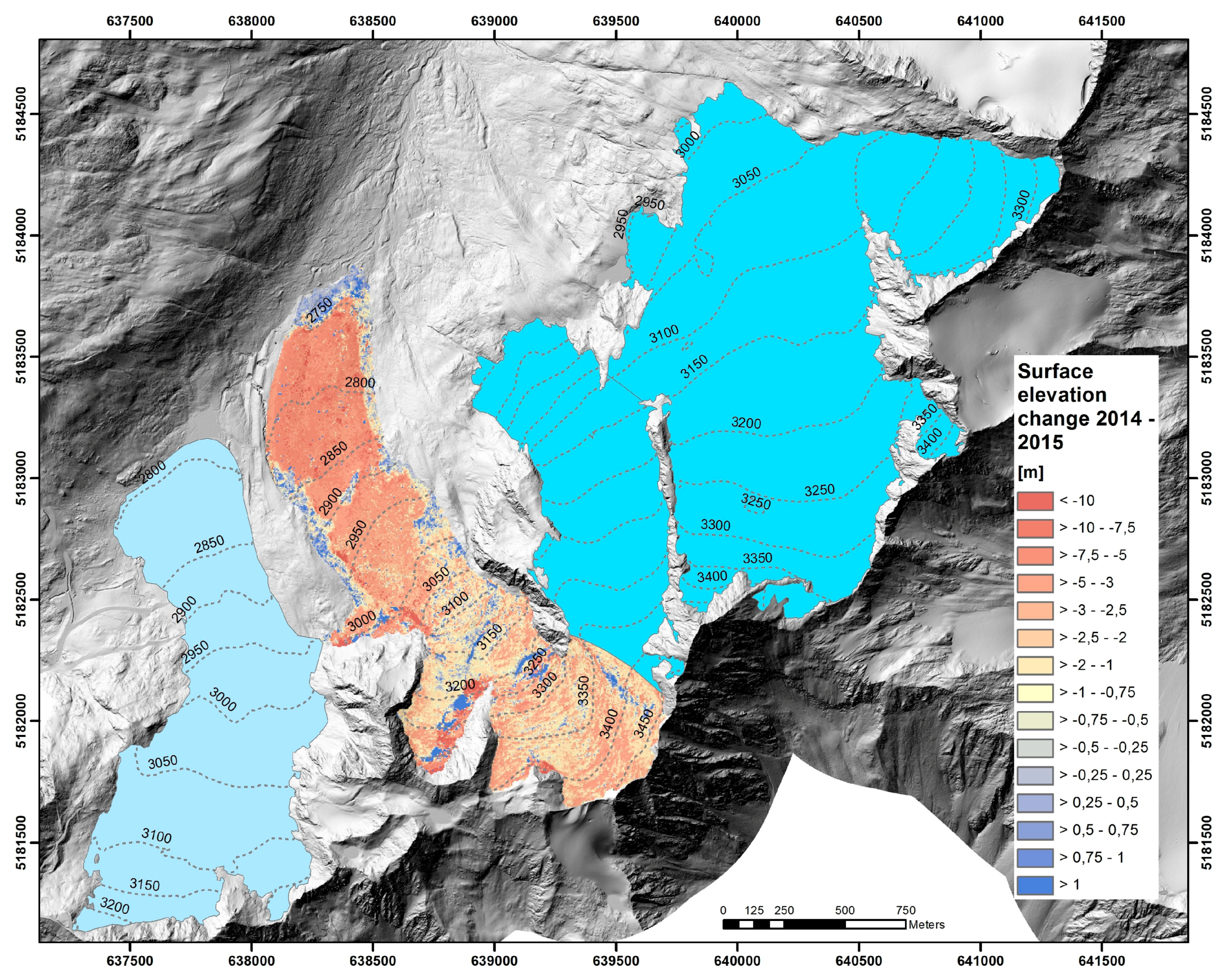
4.1. Annual Surface Elevation Change at Hochjochferner
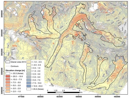
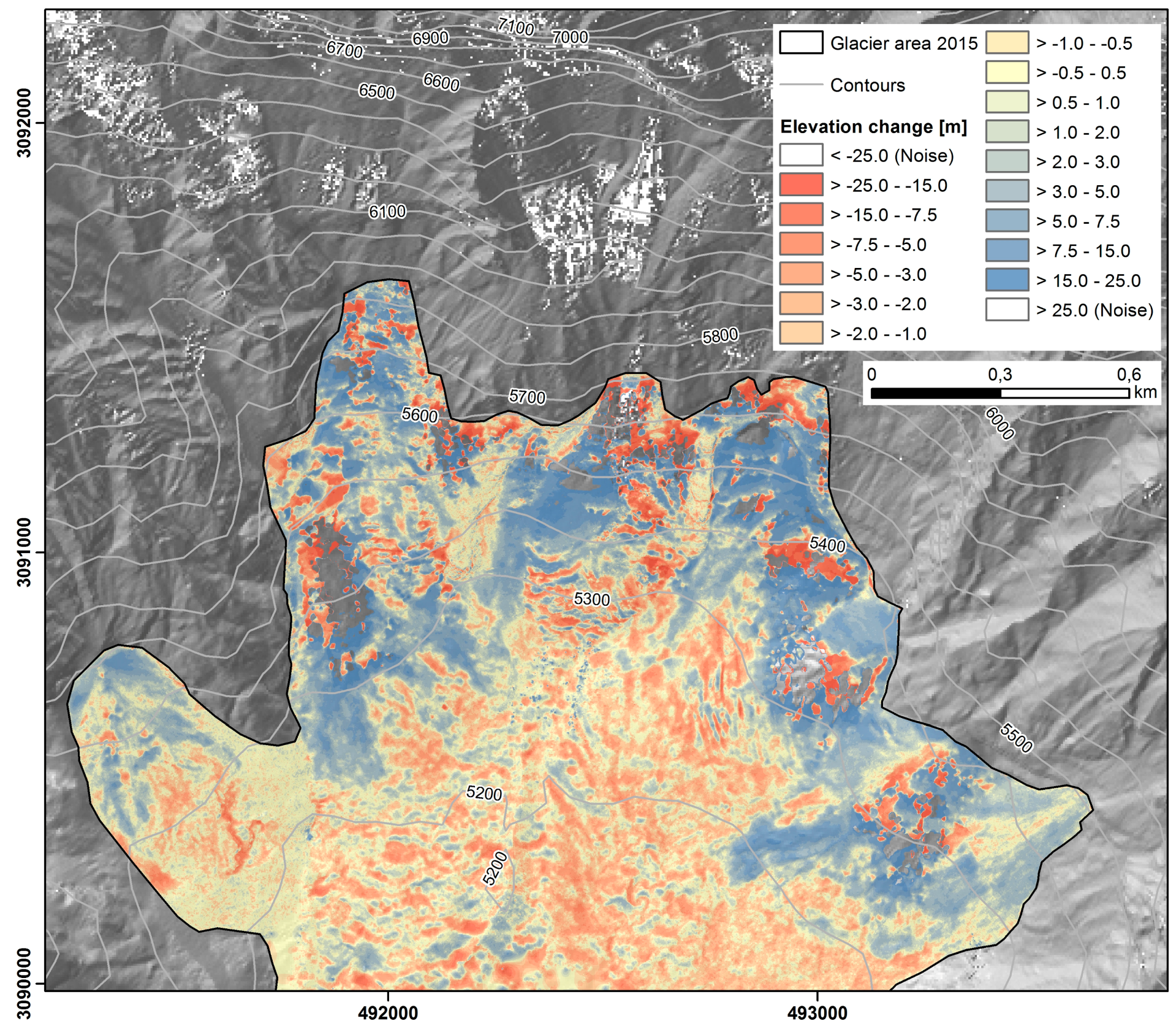
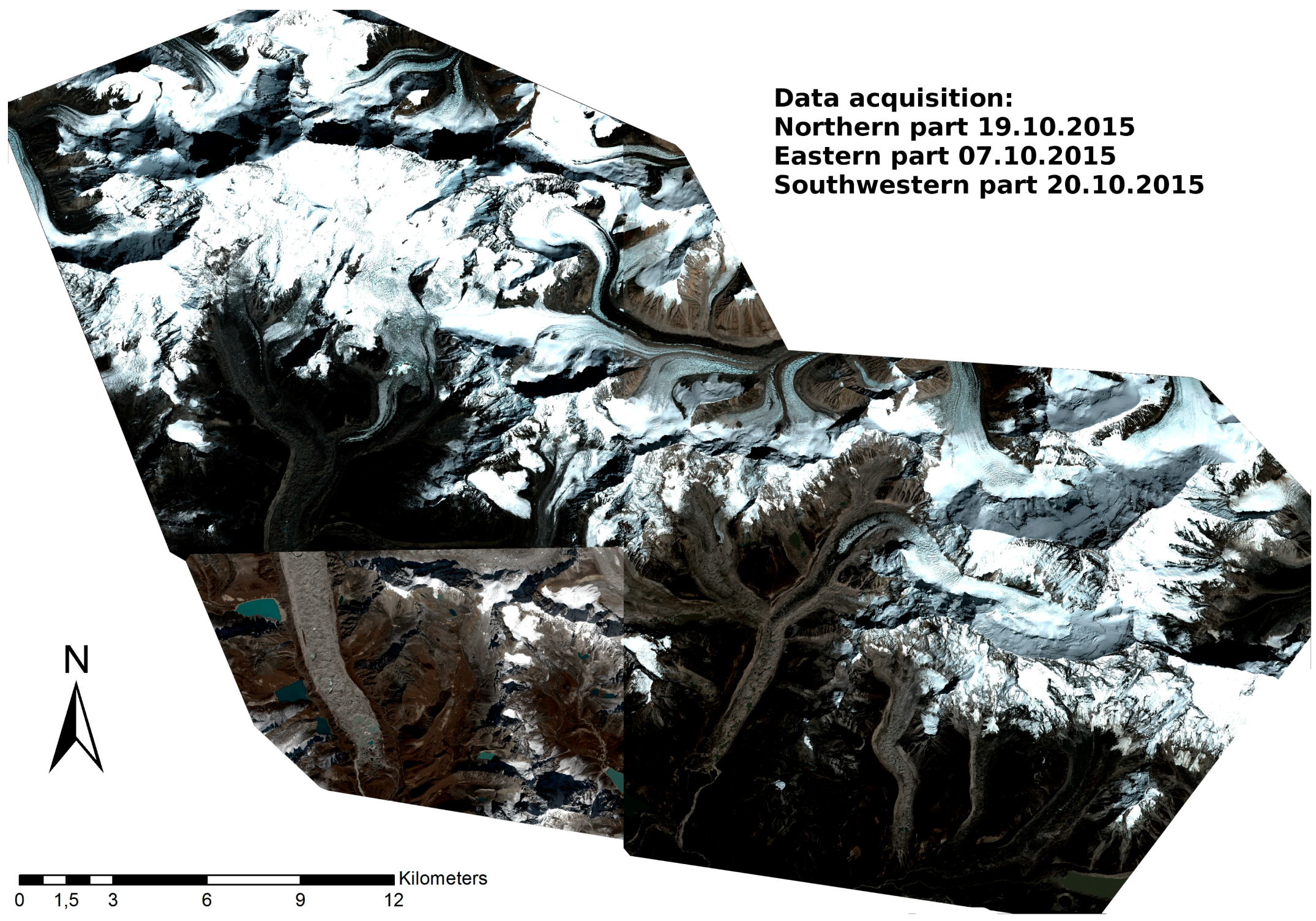
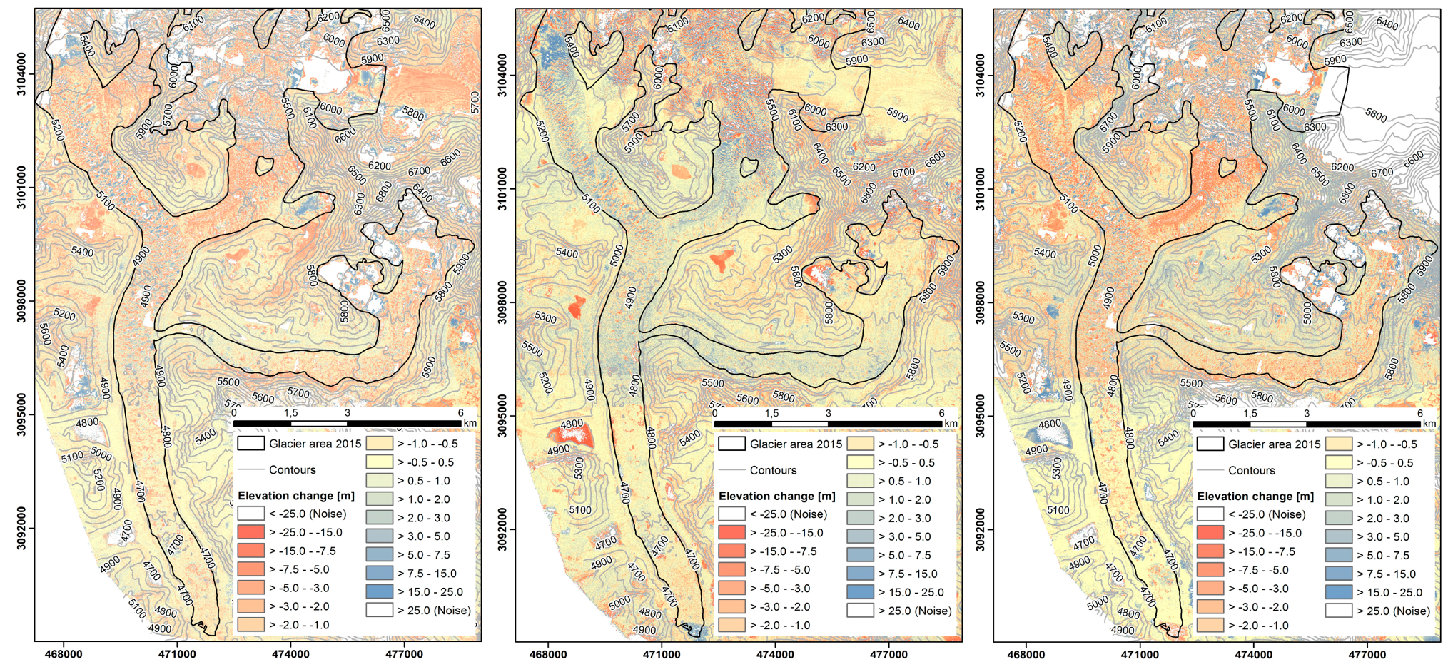
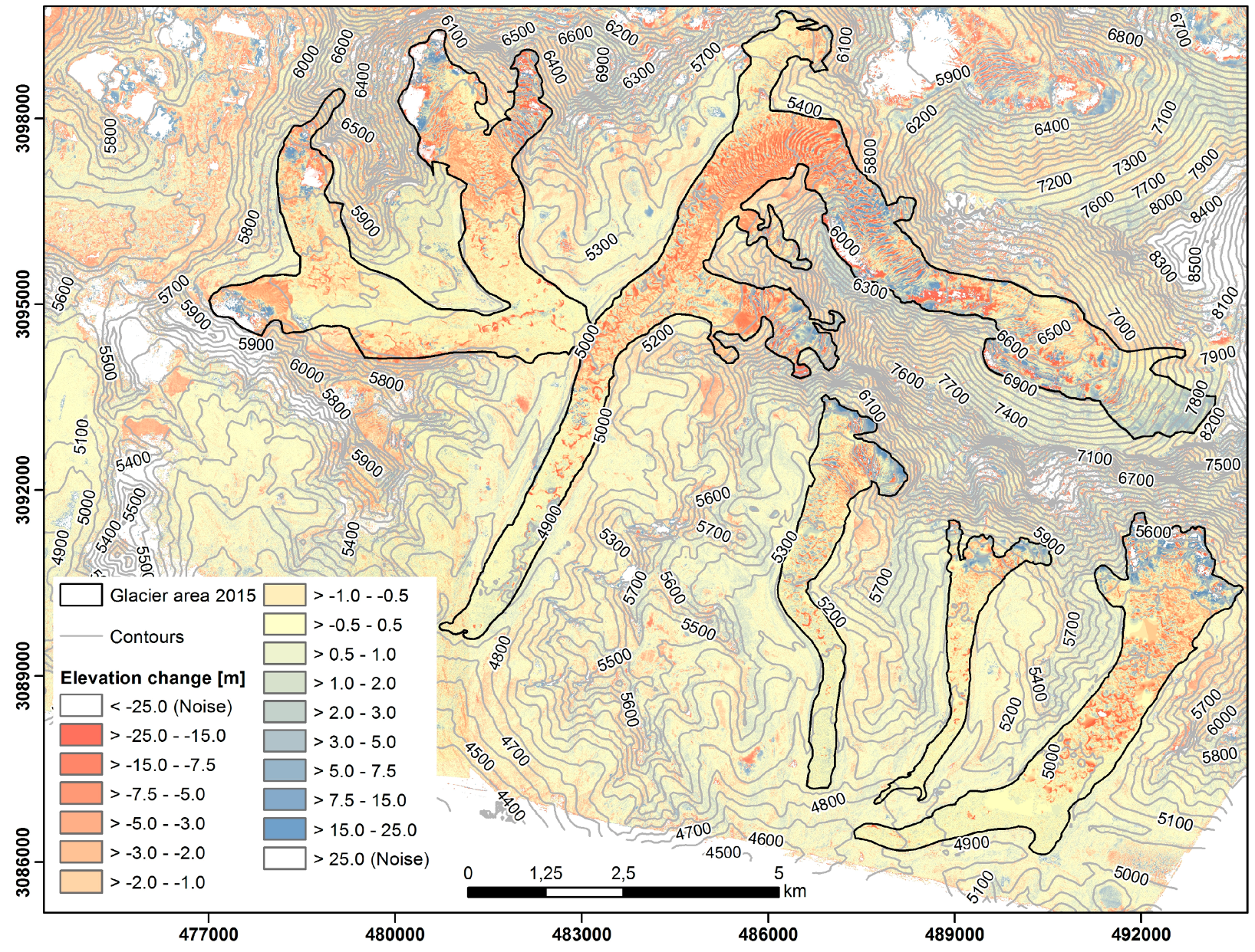
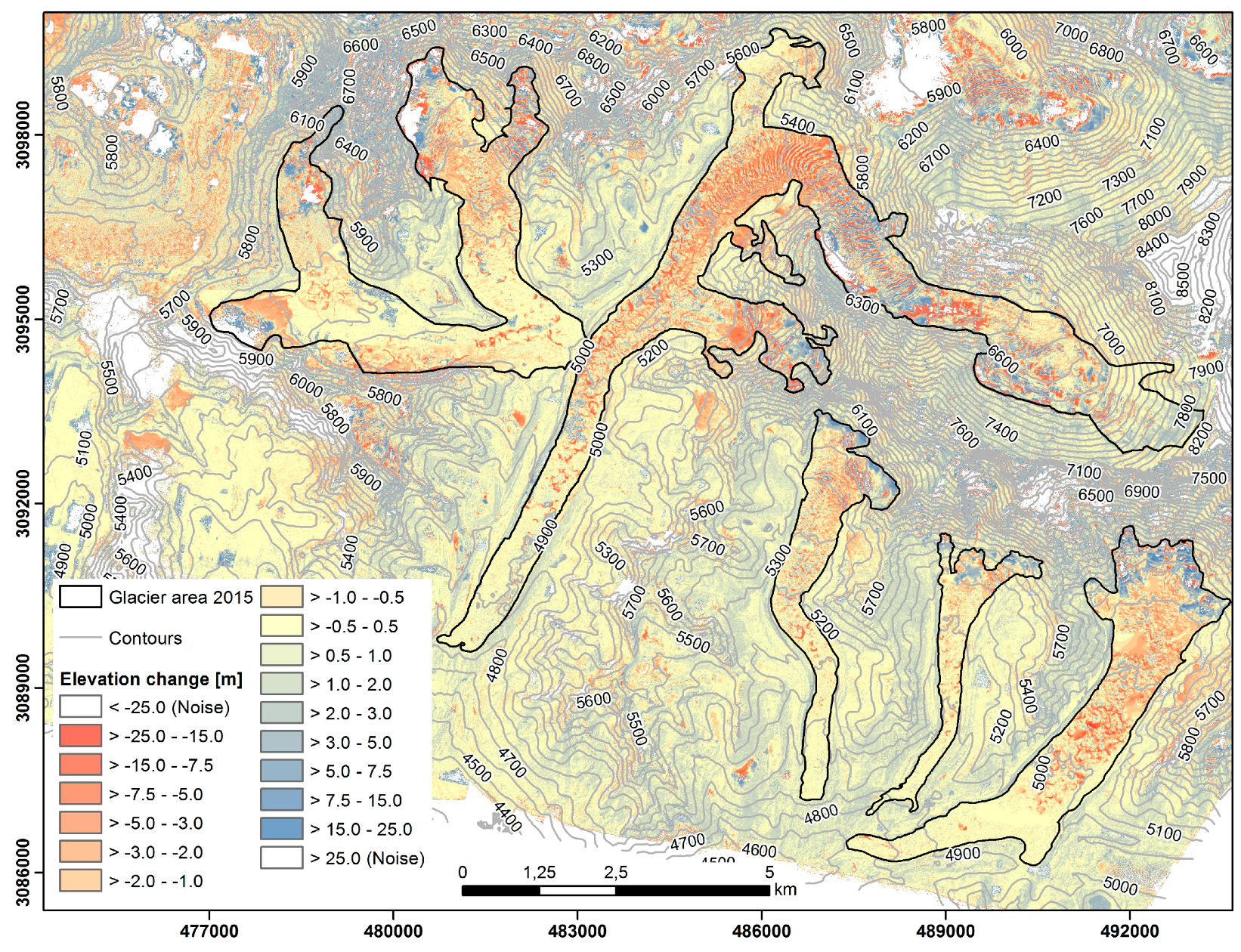
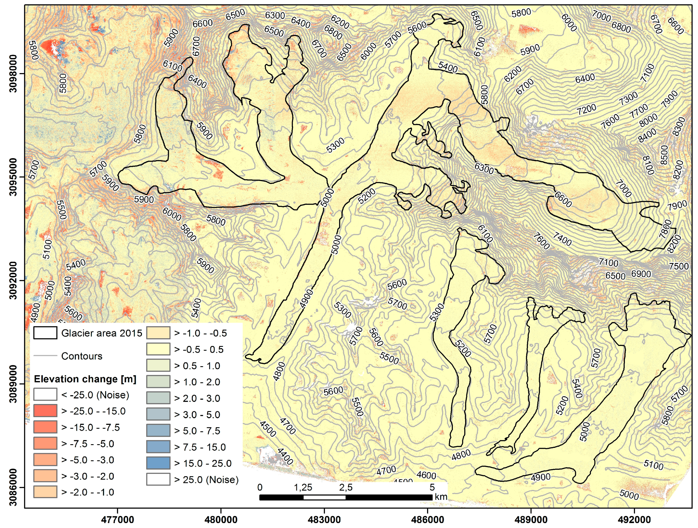
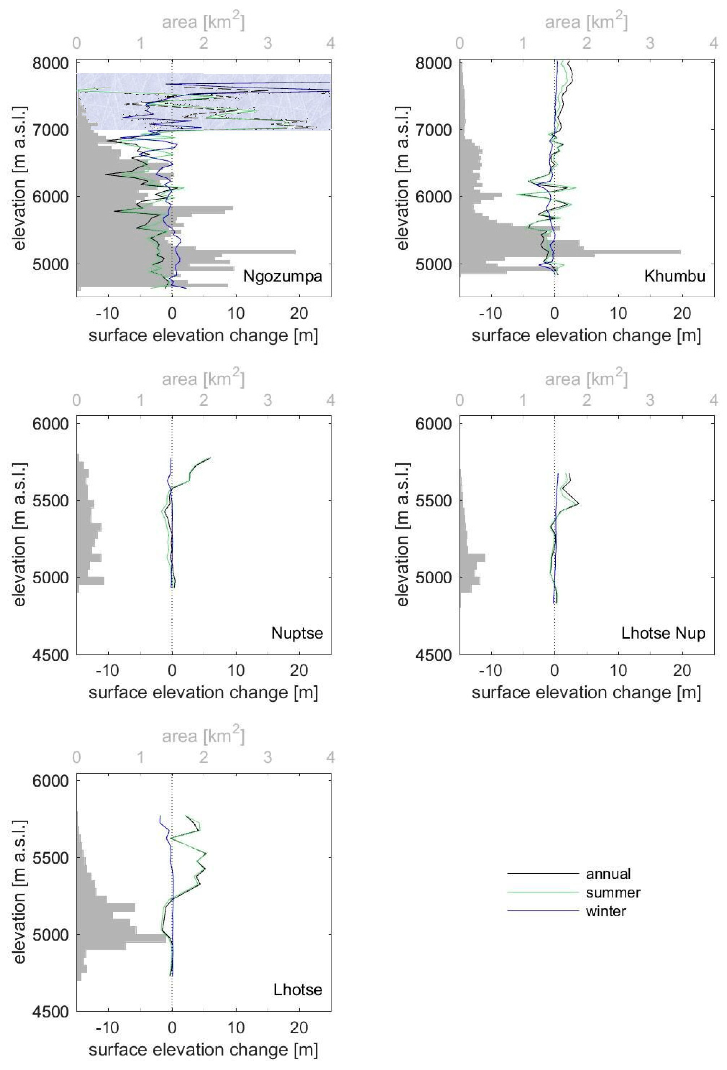
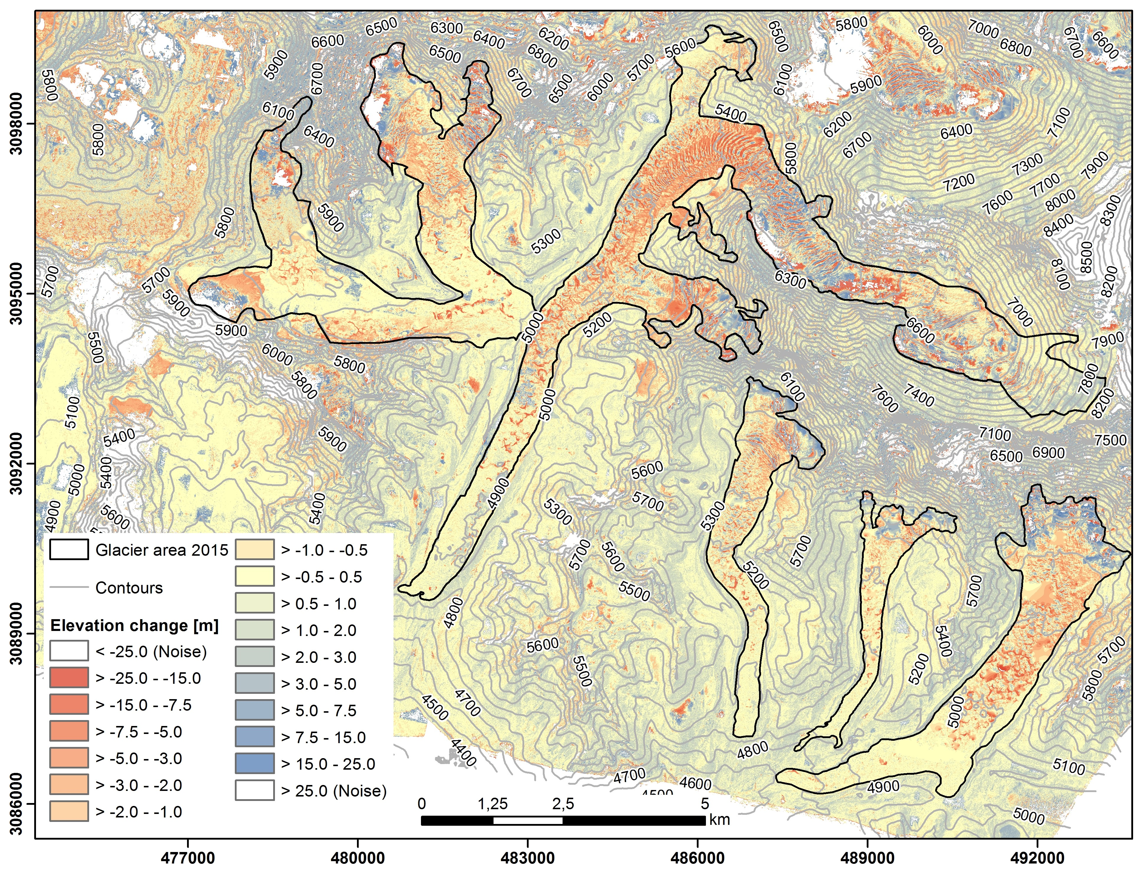
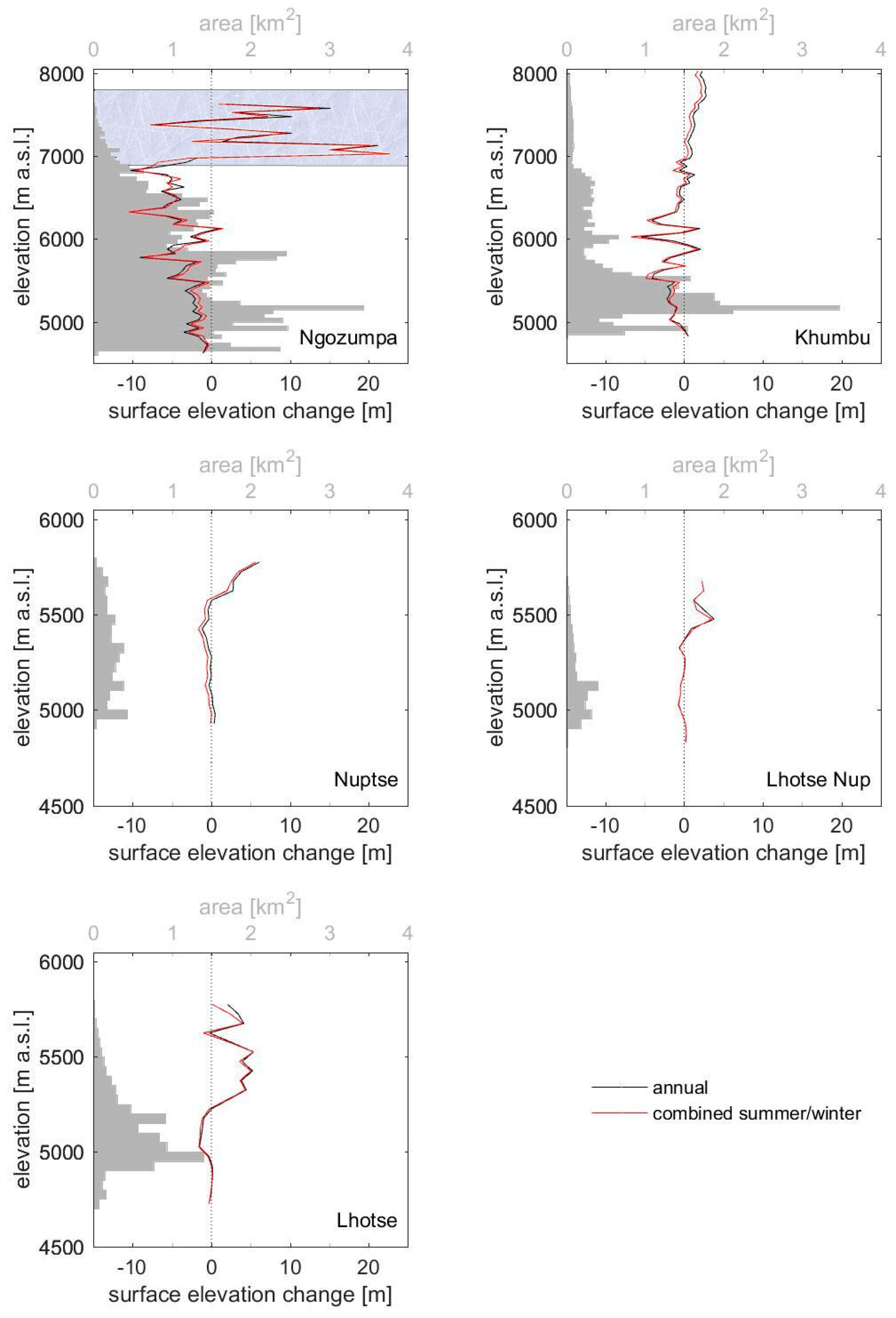
4.2. Surface Elevation Changes in the Khumbu Himal
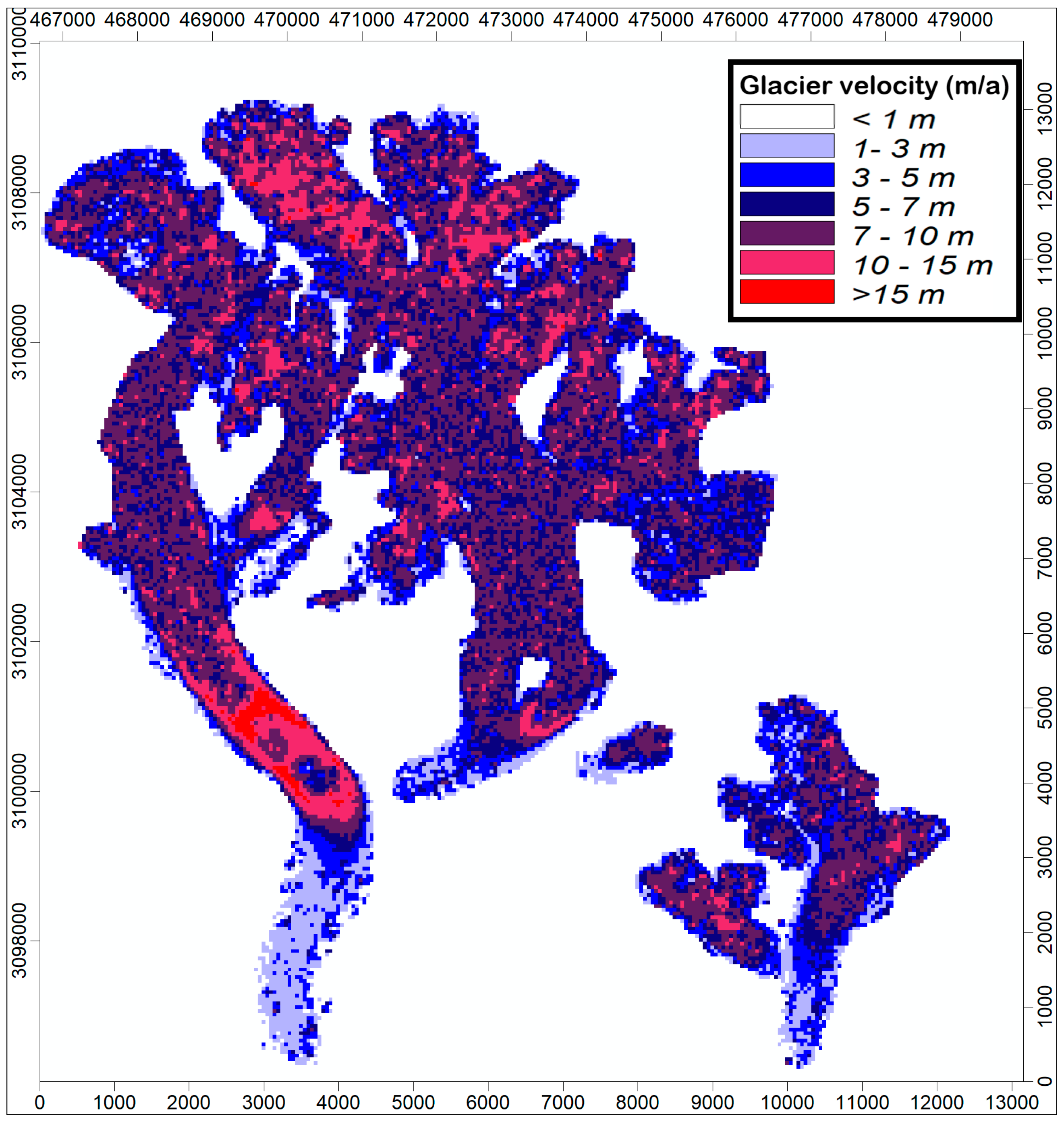
4.3. Image Correlation for Deriving Glacier Surface Velocity
5. Discussion
5.1. Problems of DEM based on Pléiades Data in High Mountain Areas
5.2. Accuracy of DEM based on Pléiades Tri-Stereo Data With and Without the Use of GCPs
5.3. Glaciological Interpretation
6. Conclusions
Author Contributions
Funding
Acknowledgments
Conflicts of Interest
References
- Bolch, T.; Buchroithner, M.; Pieczonka, T.; Kunert, A. Planimetric and volumetric glacier changes in the Khumbu Himal, Nepal, since 1962 using Corona, Landsat TM and ASTER data. J. Glaciol. 2008, 54, 592–600. [Google Scholar] [CrossRef] [Green Version]
- Nuimura, T.; Fujita, K.; Yamaguchi, S.; Sharma, R.R. Elevation changes of glaciers revealed by multitemporal digital elevation models calibrated by GPS survey in the Khumbu region, Nepal Himalaya, 1992–2008. J. Glaciol. 2012, 58, 648–656. [Google Scholar] [CrossRef]
- Racoviteanu, A.E.; Williams, M.W. Decision Tree and Texture Analysis for Mapping Debris-Covered Glaciers in the Kangchenjunga Area, Eastern Himalaya. Remote Sens. 2012, 4, 3078–3109. [Google Scholar] [CrossRef] [Green Version]
- Berthier, E.; Arnaud, Y.; Kumar, R.; Ahmad, S.; Wagnon, P.; Chevallier, P. Remote sensing estimates of glacier mass balances in the Himachal Pradesh (Western Himalaya, India). Remote Sens. Environ. 2007, 108, 327–338. [Google Scholar] [CrossRef] [Green Version]
- Belart, J.M.C.; Berthier, E.; Magnússon, E.; Anderson, L.S.; Pálsson, F.; Thorsteinsson, T.; Howat, I.M.; Aðalgeirsdóttir, G.; Jóhannesson, T.; Jarosch, A.H. Winter mass balance of Drangajökull ice cap (NW Iceland) derived from satellite sub-meter stereo images. Cryosphere 2017, 11, 1501–1517. [Google Scholar] [CrossRef] [Green Version]
- Bolch, T.; Pieczonka, T.; Benn, D.I. Multi-decadal mass loss of glaciers in the Everest area (Nepal Himalaya) derived from stereo imagery. Cryosphere 2011, 5, 349–358. [Google Scholar] [CrossRef] [Green Version]
- Kääb, A.; Berthier, E.; Nuth, C.; Gardelle, J.; Arnaud, Y. Contrasting patterns of early twenty-first-century glacier mass change in the Himalayas. Nature 2012, 488, 495–498. [Google Scholar] [CrossRef] [PubMed]
- Huggel, C.; Kääb, A.; Haeberli, W.; Teysseire, P.; Paul, F. Remote sensing based assess-ment of hazards from glacier lake outbursts: A case study in the Swiss Alps. Can. Geo-Tech. J. 2002, 39, 316–330. [Google Scholar] [CrossRef]
- Wessels, R.; Kargel, J.S.; Kieffer, H.H. ASTER measurement of supraglacial lakes in the Mount Everest region of Himalaya. Ann. Glaciol. 2002, 34, 399–408. [Google Scholar] [CrossRef]
- Salzmann, N.; Kääb, A.; Huggel, C.; Allgöwer, B.; Haeberli, W. Assessment of the hazard potential of ice avalanches using remote sensing and GIS-modelling. Nor. J. Geogr. 2004, 58, 74–84. [Google Scholar] [CrossRef]
- Paul, F.; Huggel, C.; Kääb, A. Combining satellite multispectral image data and a digital elevation model for mapping debris-covered glaciers. Remote Sens. Environ. 2004, 89, 510–518. [Google Scholar] [CrossRef]
- Casey, K.; Kääb, A.; Benn, D.I. Geochemical characterization of supraglacial debris via in situ and optical remote sensing methods: A case study in Khumbu Himalaya, Nepal. Cryosphere 2012, 6, 85–100. [Google Scholar] [CrossRef] [Green Version]
- Robson, B.A.; Nuth, C.; Dahl, S.O.; Hölbling, D.; Strozzi, T.; Nielsen, P.R. Automated classification of debris-covered glaciers combining optical, SAR and topographic data in an object-based environment. Remote Sens. Environ. 2015, 170, 372–387. [Google Scholar] [CrossRef] [Green Version]
- Gleyzes, A.; Perret, L.; Kubik, P. Pleiades system architecture and main performances. Int. Arch. Photogramm. Remote Sens. Spat. Inf. Sci. 2012, 39, 537–542. [Google Scholar] [CrossRef]
- Centre National d’Etudes Spatiales. Pleiades Mission. 2016. Available online: https://Pleiades.cnes.fr/en/PLEIADES/index.htm (accessed on 31 March 2016).
- Berthier, E.; Vincent, C.; Magnússon, E.; Gunnlaugsson, Á.Þ.; Pitte, P.; Le Meur, E.; Masiokas, M.; Ruiz, L.; Pálsson, F.; Belart, J.M.C.; et al. Glacier topography and elevation changes derived from Pléiades sub-meter stereo images. Cryosphere 2014, 8, 2275–2291. [Google Scholar] [CrossRef] [Green Version]
- Wagnon, P.; Vincent, C.; Arnaud, Y.; Berthier, E.; Vuillermoz, E.; Gruber, S.; Pokhrel, B.K. Seasonal and annual mass balances of Mera and Pokalde glaciers (Nepal Himalaya) since 2007. Cryosphere 2013, 7, 1769–1786. [Google Scholar] [CrossRef] [Green Version]
- Holzer, N.; Buchroithner, M.; Gourmelen, N.; Colin, J. Suitability of a Pléiades VHR Digital Surface Model for Glacier Mass Balance Estimates at Mt. Gurla Mandhata and Mt. Geladandong (China). In Proceedings of the Pleiades Days International Conference Pléiades Days, Toulouse, France, 1–3 April 2014. [Google Scholar]
- Ruiz, L.; Berthier, E.; Masiokas, M.; Pitte, P.; Villalba, R. First surface velocity maps for glaciers of Monte Tronador, North Patagonian Andes, derived from sequential Pleiades satellite images. J. Glaciol. 2015, 61, 908–922. [Google Scholar] [CrossRef]
- Ruiz, L.; Berthier, E.; Viale, M.; Pitte, P.; Masiokas, M.H. Recent geodetic mass balances of Monte Tronador glaciers, northern Patagonian Andes. Cryosphere 2017, 11, 619–634. [Google Scholar] [CrossRef]
- Bagnardi, M.; González, P.J.; Hooper, A. High-resolution digital elevation model from tri-stereo Pléiades-1 satellite imagery for lava flow volume estimates at Fogo Volcano. Geophys. Res. Lett. 2016, 43, 6267–6275. [Google Scholar] [CrossRef]
- Poli, D.; Remondino, F.; Angiuli, E.; Agugiaro, G. Evaluation of Pléiades-1A Triplet on Trento Testfield. Int. Arch. Photogramm. Remote Sens. Spat. Inf. Sci. 2013, 287–292. [Google Scholar] [CrossRef]
- Hirschmüller, H. Stereo processing by semiglobal matching and mutual information. IEEE Trans. Pattern Anal. Mach. Intell. 2008, 30, 328–341. [Google Scholar] [CrossRef] [PubMed]
- Juen, I.; Kaser, G. Climate Data Vent, Ötztal Alps, 2012–2016. Dataset #876595; Pangea, 2017, Bremen, Germany. Available online: https://doi.pangaea.de/10.1594/PANGAEA.876595 (accessed on 21 June 2018).
- Abermann, J.; Lambrecht, A.; Fischer, A.; Kuhn, M. Quantifying trends in glacier area and volume in the Austrian Ötztal Alps (1969–1997–2006). Cryosphere 2009, 3, 205–215. [Google Scholar] [CrossRef]
- Fischer, A.; Seiser, B.; Stocker-Waldhuber, M.; Mitterer, C.; Abermann, J. Tracing glacier changes in Austria from the Little Ice Age to the present using a lidar-based high-resolution glacier inventory in Austria. Cryosphere 2015, 9, 753–766. [Google Scholar] [CrossRef] [Green Version]
- Immerzeel, W.; van Beek, L.P.H.; Bierkens, M.F.P. Climate Change Will Affect the Asian Water Towers. Science 2010, 328, 1382–1385. [Google Scholar] [CrossRef] [PubMed]
- Racoviteanu, A.E.; Williams, M.W.; Barry, R.G. Optical Remote Sensing of Glacier Characteristics: A Review with Focus on the Himalaya. Sensors 2008, 8, 3355–3383. [Google Scholar] [CrossRef] [PubMed] [Green Version]
- Bolch, T.; Kulkarni, A.; Kääb, A.; Huggel, C.; Paul, F.; Cogley, J.G.; Frey, H.; Kargel, J.S.; Fujita, K.; Scheel, M.; et al. The State and Fate of Himalayan Glaciers. Science 2012, 336, 310–314. [Google Scholar] [CrossRef] [PubMed] [Green Version]
- Salerno, F.; Thakuri, S.; Tartari, G.; Nuimura, T.; Sunako, S.; Sakai, A.; Fujita, K. Debris-covered glacier anomaly) Morphological factors controlling changes in the mass balance, surface area, terminus position, and snow line altitude of Himalayan glaciers. Earth Planet. Sci. Lett. 2017, 471, 19–31. [Google Scholar] [CrossRef]
- De Lussy, F.; Greslou, D.; Dechoz, C.; Amberg, V.; Delvit, J.M.; Lebegue, L.; Blanchet, G.; Fourest, S. Pleiades HR in flight geometrical calibration: Location and mapping of the focal plane. ISPRS Int. Arch. Photogramm. Remote Sens. Spat. Inf. Sci. 2012, 39, 519–523. [Google Scholar] [CrossRef]
- Vincent, C.; Wagnon, P.; Shea, J.M.; Immerzeel, W.W.; Kraaijenbrink, P.; Shrestha, D.; Soruco, A.; Arnaud, Y.; Brun, F.; Berthier, E.; et al. Reduced melt on debris-covered glaciers: Investigations from Changri Nup Glacier, Nepal. Cryosphere 2016, 10, 1845–1858. [Google Scholar] [CrossRef] [Green Version]
- Perko, R.; Raggam, H.; Gutjahr, K.H.; Schardt, M. Assessment of the mapping potential of Pléiades stereo and triplet data. ISPRS Int. Arch. Photogramm. Remote Sens. Spat. Inf. Sci. 2014, 103–109. [Google Scholar] [CrossRef]
- Haala, N. Comeback of Digital Image Matching. In Proceedings of the 52nd Photogrammetric Week, Stuttgart, Germany, 7–11 September 2009; Wichmann Verlag: Berlin, Germany, 2009; pp. 289–301. [Google Scholar]
- Tiris. Digitale Orthofotos Tirol. 2013; Dataset identifier: 49FB0C5C-1CDC-40C3-98D6-0598D0CD5864. [Google Scholar]
- Eisank, C.; Rieg, L.; Klug, C.; Kleindienst, H.; Sailer, R. Semi-Global Matching of Pléiades Tri-Stereo Imagery to Generate Detailed Digital Topography for High-Alpine Regions. In Proceedings of the GI-Forum, Salzburg, Austria, 7–10 July 2015. [Google Scholar]
- Galos, S.P.; Klug, C.; Prinz, R.; Rieg, L.; Dinale, R.; Sailer, R.; Kaser, G. Recent glacier changes and related contribution potential to river discharge in the Vinschau/Val Venosta, Italian Alps. Geogr. Fis. Dinam. Quat. 2015, 38, 143–154. [Google Scholar] [CrossRef]
- Rieg, L.; Wichmann, V.; Rutzinger, M.; Sailer, R.; Geist, T.; Stötter, J. Datainfrastructure for multitemporal airborne LiDAR point cloud analysis—Examples from physical geography in high mountain environments. Computers, Environment and Urban Systems Special Issue: 3D Laser Scanning. Spat. Data Anal. Infrastruct. 2014, 45, 137–146. [Google Scholar] [CrossRef]
- Sailer, R.; Rutzinger, M.; Rieg, L.; Wichmann, V. Digital elevation models derived from airborne laser scanning point clouds: Appropriate spatial resolutions for multi-temporal characterization and quantification of geomorphological processes. Earth Surf. Proc. Landf. 2013. [Google Scholar] [CrossRef]
- Klug, C.; Rieg, L.; Ott, P.; Mössinger, M.; Sailer, R.; Stötter, J. A Multi-Methodological Approach to Determine Permafrost Occurrence and Ground Surface Subsidence in Mountain Terrain, Tyrol, Austria. Perm. Perig. Proc. 2016, 28, 249–265. [Google Scholar] [CrossRef] [Green Version]
- Nuth, C.; Kääb, A. Co-registration and bias corrections of satellite elevation data sets for quantifying glacier thickness change. Cryosphere 2011, 5, 271–290. [Google Scholar] [CrossRef] [Green Version]
- Berthier, E. On the use of Pléiades imagery in glaciology. DEM generation and velocity mapping. 2. In Proceedings of the Pleiades Days International Conference Pléiades Days, Toulouse, France, 1–3 April 2014. [Google Scholar]
- Scambos, T.A.; Dutkiewitcz, M.J.; Wilson, J.C.; Bindschadler, R.A. Application of image cross-correlation software to the measurement of glacier velocity using satellite data. Remote Sens. Environ. 1992, 42, 177–186. [Google Scholar] [CrossRef]
- Lambrecht, A.; Kuhn, M. Glacier Changes in the Austrian Alps During the Last Three Decades, Derived from the New Austrian Glacier Inventory. Ann. Glaciol. 2007, 46, 177–184. [Google Scholar] [CrossRef]
- Carturan, L.; Filippi, R.; Seppi, R.; Gabrielli, P.; Notarnicola, C.; Bertoldi, L.; Paul, F.; Rastner, P.; Cazorzi, F.; Dinale, R.; et al. Area and volume loss of the glaciers in the Ortles-Cevedale group (Eastern Italian Alps): Controls and imbalance of the remaining glaciers. Cryosphere 2013, 7, 1339–1359. [Google Scholar] [CrossRef] [Green Version]
- Ageta, Y.; Higuchi, K. Estimation of Mass Balance Components of a Summer-Accumulation Type Glacier in the Nepal Himalaya. Geogr. Ann. Ser. A Phys. Geogr. 1984, 66, 249–255. [Google Scholar] [CrossRef]
- Fujita, K.; Ageta, Y. Effect of summer accumulation on glacier mass balance on the Tibetan Plateau revealed by mass-balance model. J. Glaciol. 2000, 46, 153–244. [Google Scholar] [CrossRef]
- Salerno, F.; Guyennon, N.; Thakuri, S.; Viviano, G.; Romano, E.; Vuillermoz, E.; Cristofanelli, P.; Stocchi, P.; Agrillo, G.; Ma, Y.; et al. Weak precipitation, warm winters and Springs impact glaciers of south slopes of Mt. Everest (central Himalaya) in the last 2 decades (1994–2013). Cryopshere 2015, 9, 1229–1247. [Google Scholar] [CrossRef]
- Quincey, D.J.; Luckman, A.; Benn, D. Quantification of Everest region glacier velocities between 1992 and 2002, using satellite radar interferometry and feature tracking. J. Glaciol. 2009, 55, 596–606. [Google Scholar] [CrossRef]
- Benn, D.; Thompson, S.; Gulley, J.; Mertes, J.; Luckman, A.; Nicholson, L. Structure and evolution of the drainage system of a Himalayan debris-covered glacier, and its relationship with patterns of mass loss. Cryosphere 2017, 11, 2247–2264. [Google Scholar] [CrossRef] [Green Version]


| Acquisition | Acquisition Dates |
|---|---|
| European Alps 2014 | 23 September 2014 |
| European Alps 2015 | 21 September 2015 |
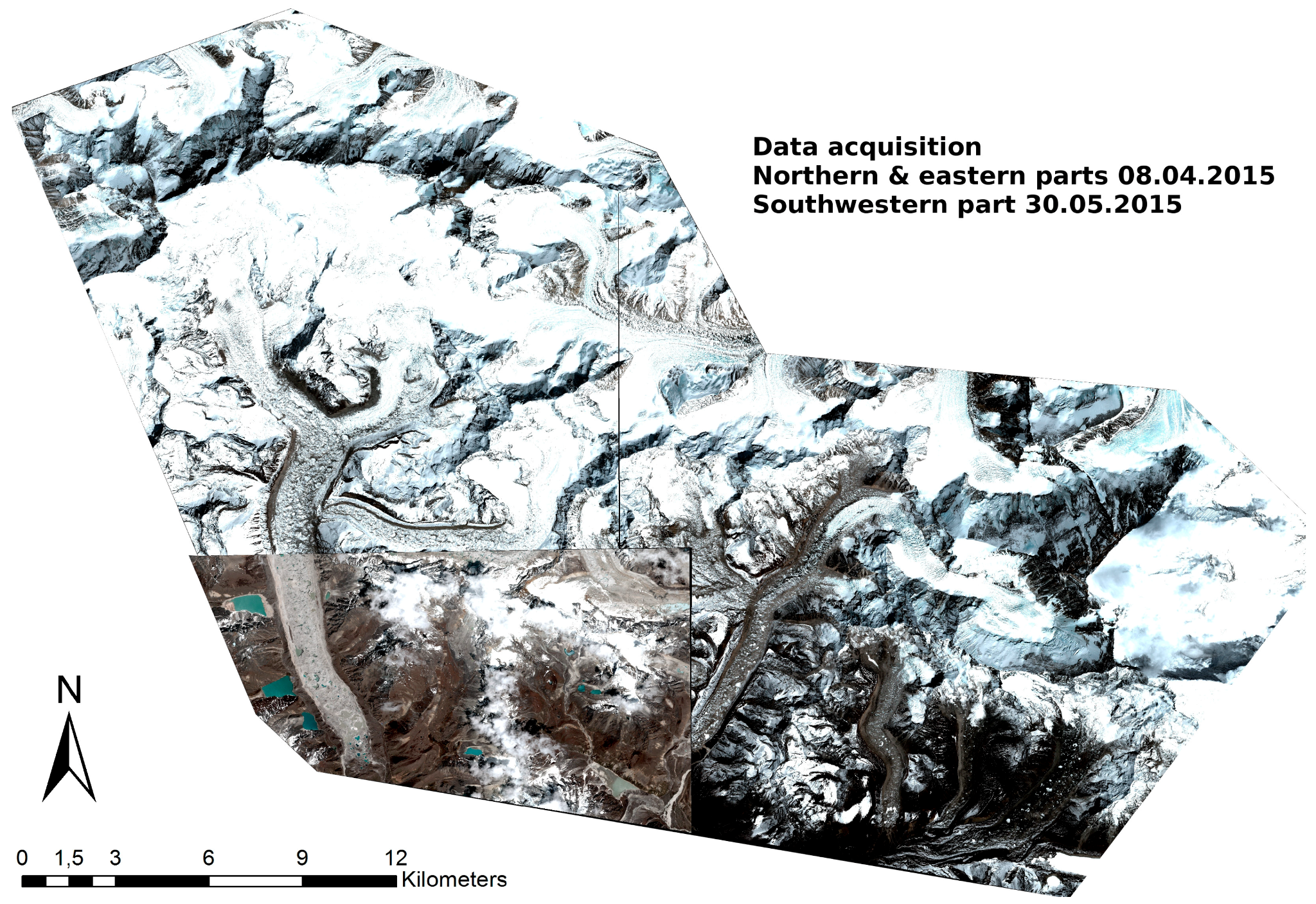
| Khumbu Himal Spring 2015 | 8 April and 30 May 2015 |
| Khumbu Himal Autumn 2015 | 7, 29, and 20 October 2015 |
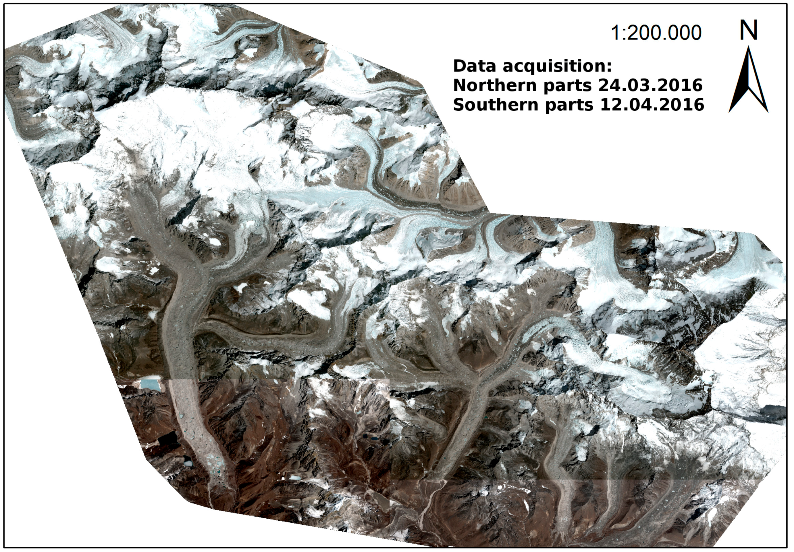
| Khumbu Himal Spring 2016 | 24 March and 12 April 2016 |
| Acquisition | Shift in x [m] | Shift in y [m] | Shift in z [m] |
|---|---|---|---|
| Alps 2014–ALS 2013 | 0.1 | −3.2 | 0.6 |
| Alps 2015–ALS 2013 | 0.2 | −2.4 | 0.5 |
| Khumbu Spring 2015–Khumbu 2016 East | 1.0 | −0.2 | −0.1 |
| Khumbu Spring 2015–Khumbu 2016 Northwest | 4.0 | −0.1 | 0.7 |
| Khumbu Spring 2015–Khumbu 2016 Southwest | 1.5 | −0.6 | 0.3 |
| Khumbu Autumn 2015–Khumbu 2016 East | 0.0 | −0.2 | 0.5 |
| Khumbu Autumn 2015–Khumbu 2016 Northwest | 1.1 | 1.8 | −3.9 |
| Khumbu Autumn 2015–Khumbu 2016 Northwest | −3.9 | −1.4 | 4.8 |
| Acquisition | Standard Deviation |
|---|---|
| Spring 2015–Spring 2016 | 1.18 |
| Spring 2015–Autumn 2015 | 0.42 |
| Autumn 2015–Spring 2016 | 0.43 |
| ID | Name | Offset x [m] | Offset y [m] | Combined Horizontal Offset [m] | Offset [z] |
|---|---|---|---|---|---|
| 1 | Boulder (N of Gokyo) | −1.2 | −0.4 | 1.3 | −6.2 |
| 2 | Gokyo Ri | 0.1 | −0.5 | 0.5 | −5.8 |
| 3 | Dragnag 1 | −1.9 | 0.8 | 2.1 | 4.2 |
| 4 | Dragnag 2 | 1.7 | −0.6 | 1.8 | −2.3 |
| 5 | Gokyo | −1.2 | 0.3 | 1.2 | −4.1 |
| 6 | Gokyo hospital | 0.6 | −2.2 | 2.3 | −4.4 |
| 7 | Ruin (S of Gokyo) | −2.2 | 1.1 | 2.5 | −1.3 |
| Glacier | Ngozumpa | Khumbu | Lhotse Nup | Nuptse | Lhotse |
|---|---|---|---|---|---|
| Area (km2) | 68.4 | 31.6 | 2.2 | 4 | 7.7 |
| Total volume change summer 2015 (km3) | −0.16134 | −0.0303 | −0.0003 | −0.00062 | −0.00125 |
| Average surface elevation change summer 2015 (m) | −2.36 | −0.96 | −0.14 | −0.16 | −0.16 |
| Total volume change winter 2015/2016 (km3) | −0.01712 | −0.0149 | 0.00024 | −0.0002 | 0.00079 |
| Average surface elevation change winter 2015/2016 (m) | −0.25 | −0.47 | 0.11 | −0.05 | 0.1 |
| Total volume change one year (km3) | −0.20609 | −0.04285 | −0.0003 | 0.00099 | 0.00065 |
| Average surface elevation change one year (m) | −0.30 | −1.35 | −0.01 | 0.25 | 0.08 |
© 2018 by the authors. Licensee MDPI, Basel, Switzerland. This article is an open access article distributed under the terms and conditions of the Creative Commons Attribution (CC BY) license (http://creativecommons.org/licenses/by/4.0/).
Share and Cite
Rieg, L.; Klug, C.; Nicholson, L.; Sailer, R. Pléiades Tri-Stereo Data for Glacier Investigations—Examples from the European Alps and the Khumbu Himal. Remote Sens. 2018, 10, 1563. https://doi.org/10.3390/rs10101563
Rieg L, Klug C, Nicholson L, Sailer R. Pléiades Tri-Stereo Data for Glacier Investigations—Examples from the European Alps and the Khumbu Himal. Remote Sensing. 2018; 10(10):1563. https://doi.org/10.3390/rs10101563
Chicago/Turabian StyleRieg, Lorenzo, Christoph Klug, Lindsey Nicholson, and Rudolf Sailer. 2018. "Pléiades Tri-Stereo Data for Glacier Investigations—Examples from the European Alps and the Khumbu Himal" Remote Sensing 10, no. 10: 1563. https://doi.org/10.3390/rs10101563