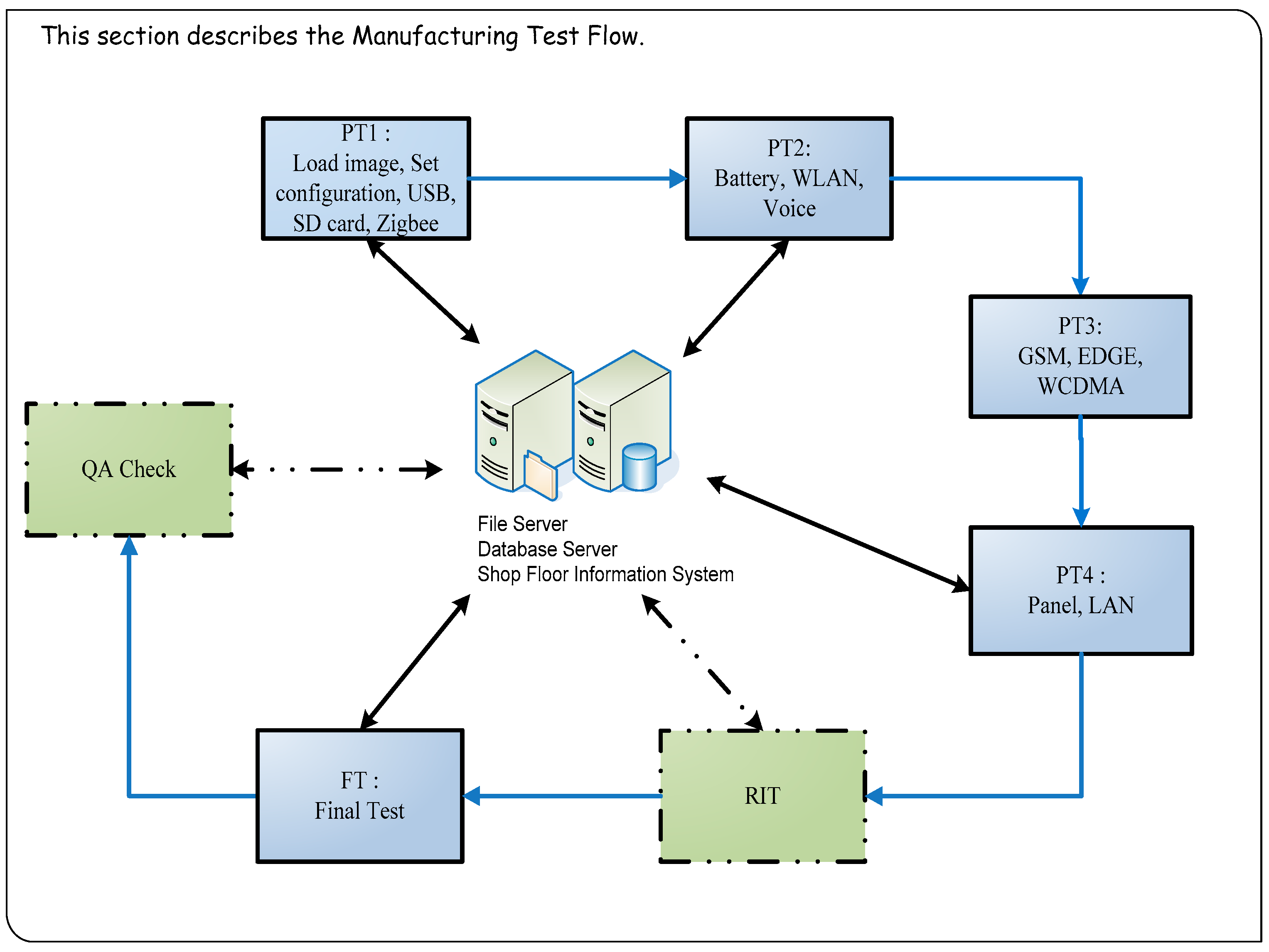
2.1. Tablet PC Testing Process
The required test items are entirely different for each stage of the testing process. Tablet PC production test process includes PT1 (Pre-Test station 1) → PT2 → PT3 → PT4 → RIT (Run-in Test) → FT (Final Test) → QA (Quality Assurance) Check (
Figure 2). At the production testing stage, tablet PCs are tested through production verification, functional testing, run-in, and volume production testing. Functional testing in particular accounts for a substantial portion of the overall production time. Therefore, functional testing was primarily investigated and improved in this study.
Currently, functional testing is extremely complex and certain content is repeated during both early and final testing. In addition, when faults occur during functional testing, the few devices analyzed and repaired during early testing are re-identified as faulty during the final testing. The MTS, logistic regression, and neural networks were employed in this study to identify more reasonable test items. High-quality engineering practices and professional engineering background knowledge were used to identify suitable test items while ensuring identical production quality [
9,
10].
2.2. MTS
The MTS is a classification technology devised by Dr. Genichi Taguchi for conducting diagnoses and forecasting with multivariate data [
11,
12]. It combines quality engineering principles and utilizes the Mahalanobis distance for the structured induction of data, serving as a basis for decision-making [
13].
Mahalanobis space is established using
k characteristic variables (
X1,
X2, …,
Xk) derived from
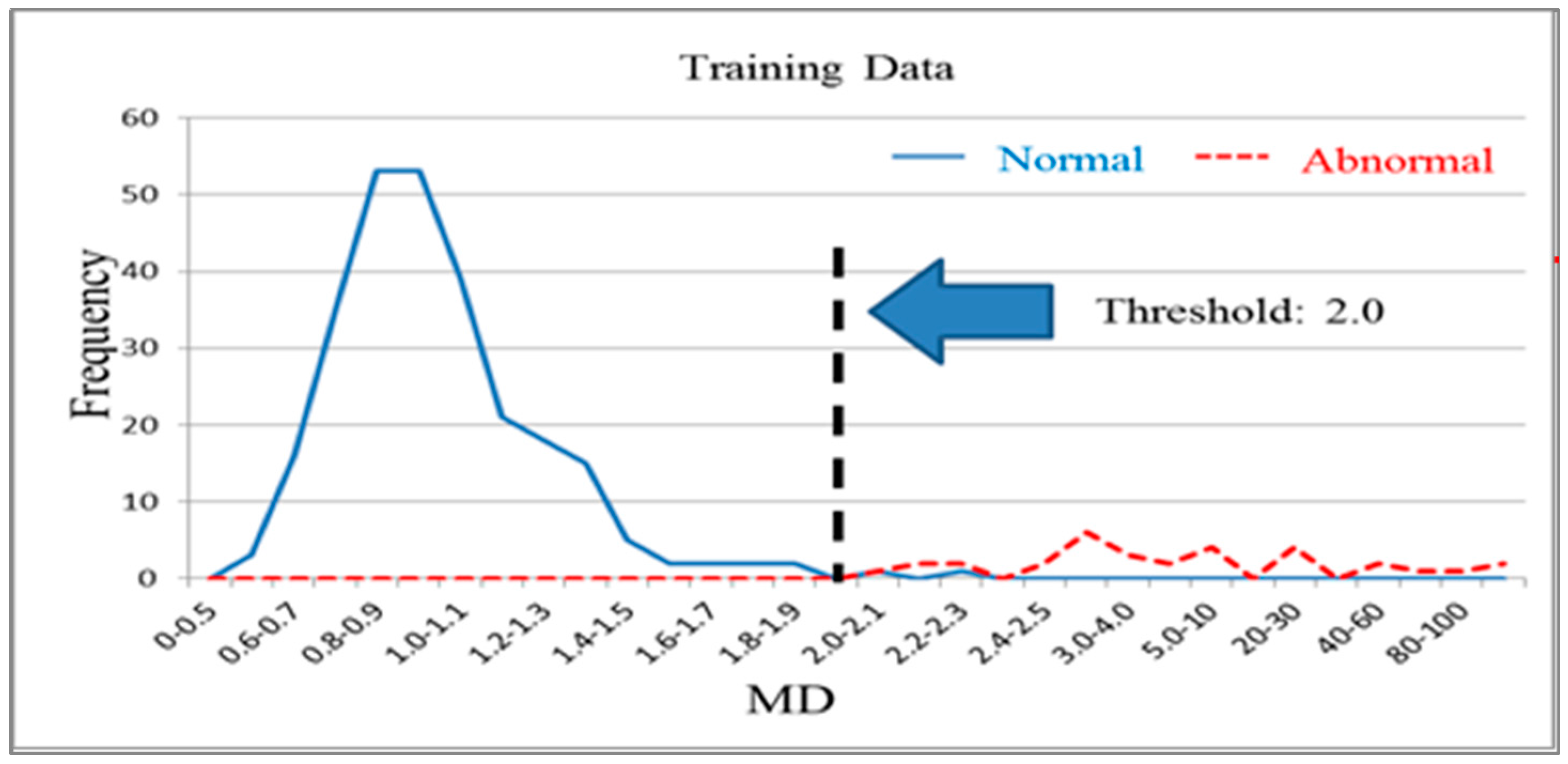
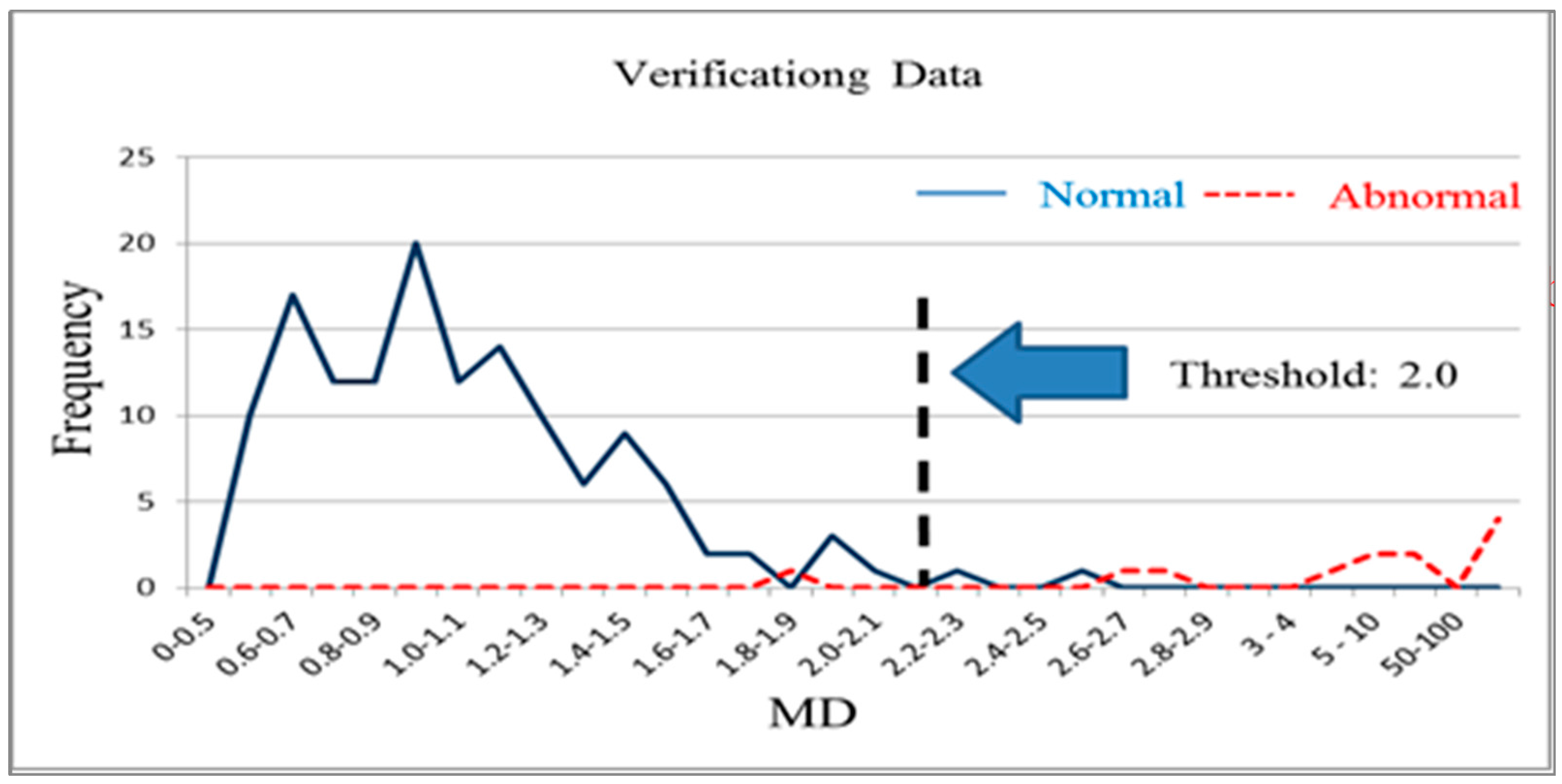
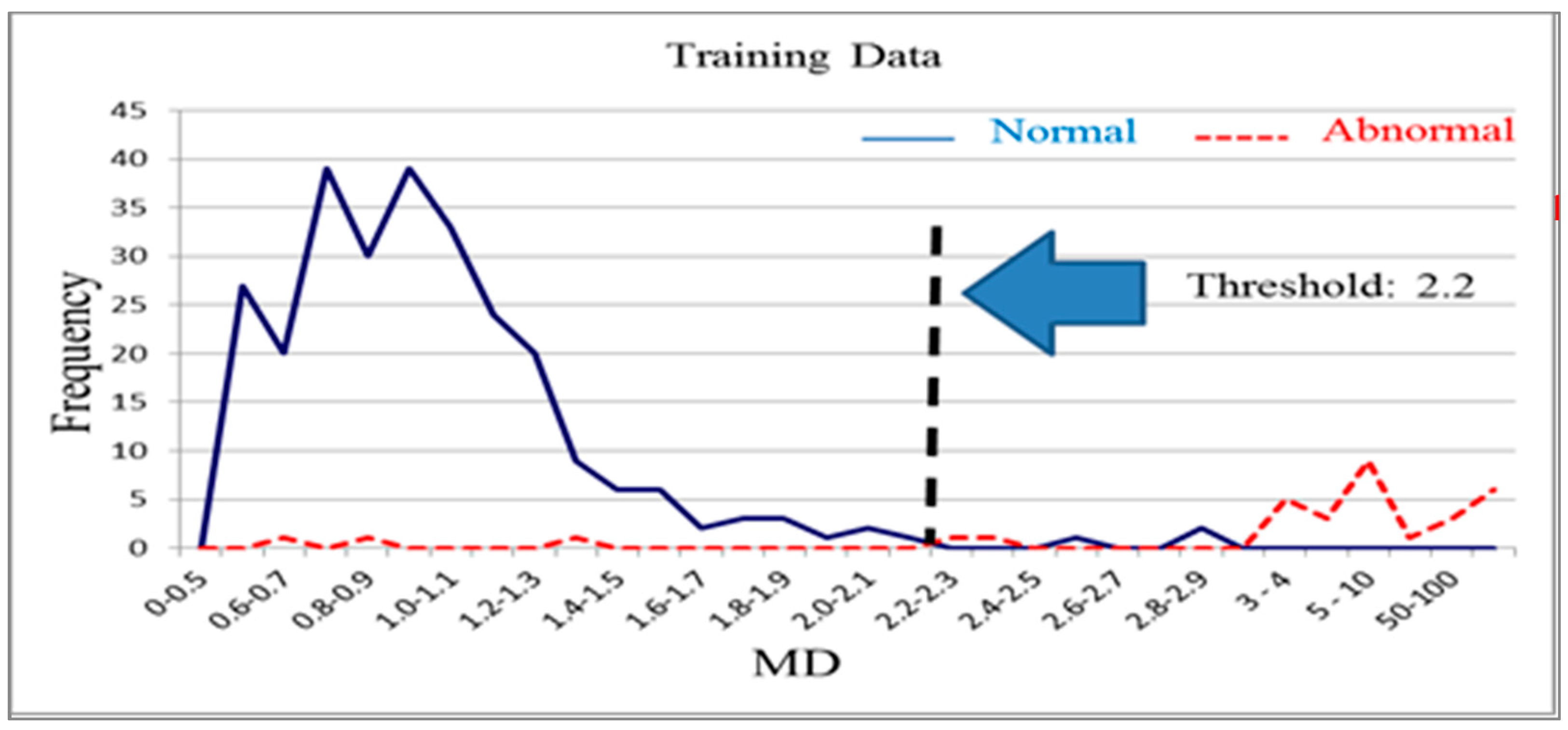
n normal products. It is used to distinguish normal products and abnormal products. The Mahalanobis distance calculated using a normal sample population has a mean approaching 1 and forms Mahalanobis space, which is also called base space. Mahalanobis space can be considered a database that includes characteristic variable means, standard deviations, and correlation coefficient inverse matrices for the normal population. Generally, the Mahalanobis distances of normal samples are less than 2.5, with values over 4 being extremely rare [
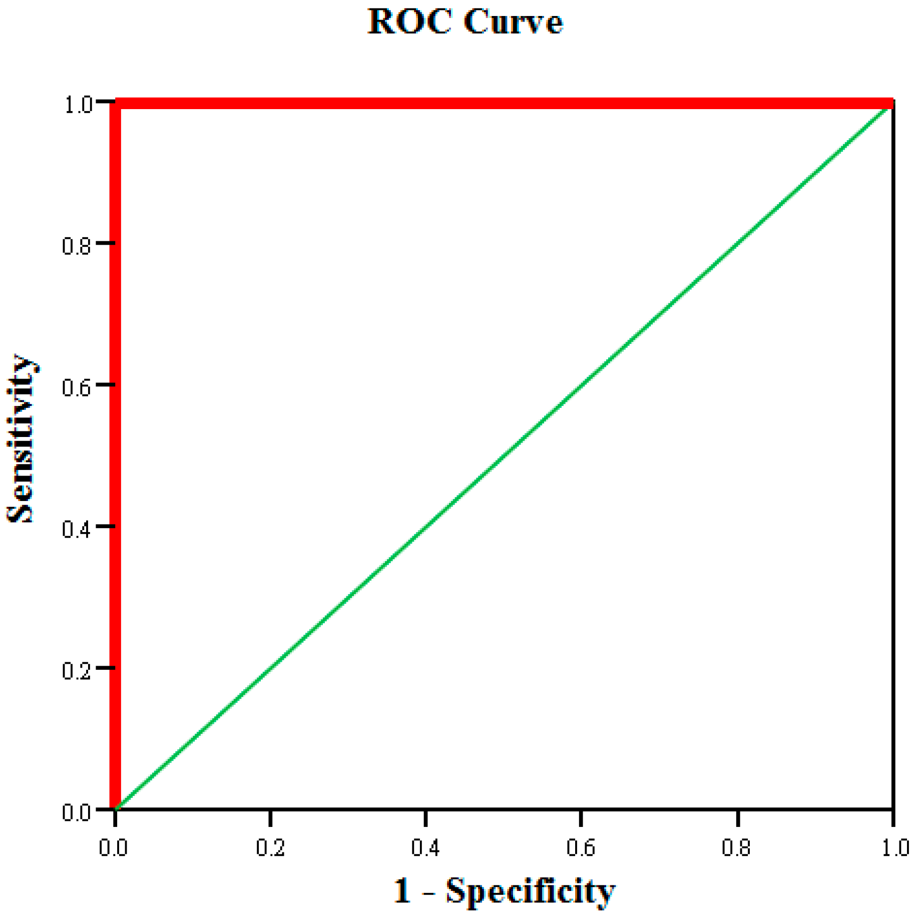
14]. The Mahalanobis distance of a product from an abnormal sample that is calculated using the means, standard deviations, and correlation coefficient inverse matrices of base space is extremely high. Additionally, thresholds can be determined using the smallest type-I error (normal products misjudged as abnormal products) and type-II errors (abnormal products misjudged as normal products) that occur [
15,
16].
In robust design, targets in orthogonal arrays are used to minimize the number of tests. This minimal test number is used to obtain reliable factor effect estimates. In the MTS, orthogonal arrays verify useful variables using the minimal number of tests [
17,
18]. Within an orthogonal array, each characteristic variable or factor is placed in a different row. Each row is a combination of different variables or factor levels representing a test combination. By using orthogonal arrays, the influence of each characteristic variable on system output can be investigated [
19,
20]. A multivariate system was assumed to have
k characteristic variables, and each characteristic variable was set to one of two levels:
The case analyzed in this study had 56 characteristic variables (
X1–
X56) that were used for analysis. Therefore, an
L64(2
63) orthogonal array with an experimental configuration. Subsequently, the Mahalanobis space established by all of the characteristic variables in the normal sample was used to calculate the Mahalanobis distance of
d abnormal samples (Equations (1)–(3)). This Mahalanobis distance was then used to obtain the signal-to-noise (SN) ratio [
21,
22].
Standardized equation:
where
Inverse correlation matrix:
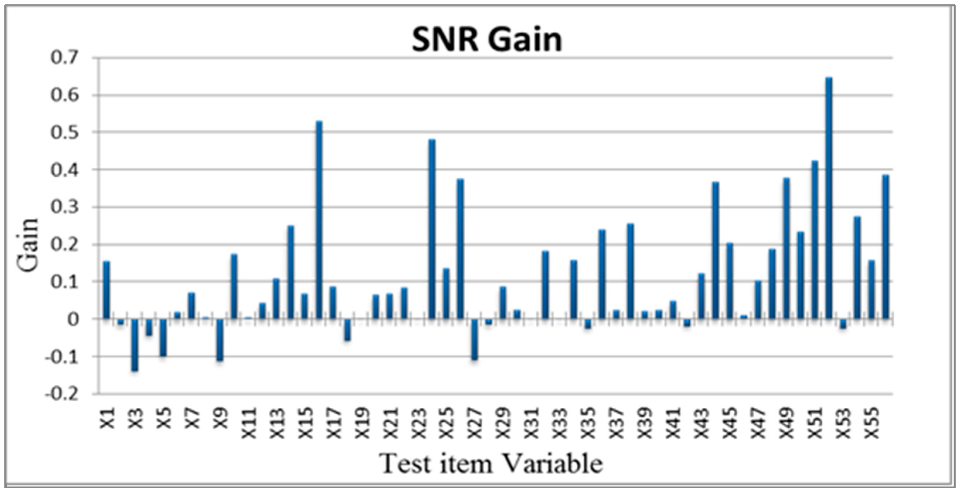
After constructing the Mahalanobis space based on the characteristic variable combinations in the orthogonal array, the SN ratio were used to select important variables. In quality engineering, the SN ratio is used as an evaluation tool with decibels as a unit. The SN ratio is used to evaluate performance using the ratio of useful information to harmful information. In multivariate analysis, confirming that a combination of variables can fully detect abnormal levels is critical.
In this study, the level of abnormality in faulty tablet PCs was tested to serve as a basis for screening test items. The larger-the-better SN ratio was used in expectation that greater Mahalanobis distances within the abnormal sample observations in relation to those of the normal sample were favorable (Equation (4)).
Assuming that greater increases in Mahalanobis distances (average SN ratio of level 1 minus average SN ratio of level 2) were favorable, the importance of the characteristic variables to the classification and diagnostic system was determined to select optimal conditions (Equation (5)).
Additionally, the selected optimal variables were used to construct reduced models [
23,
24,
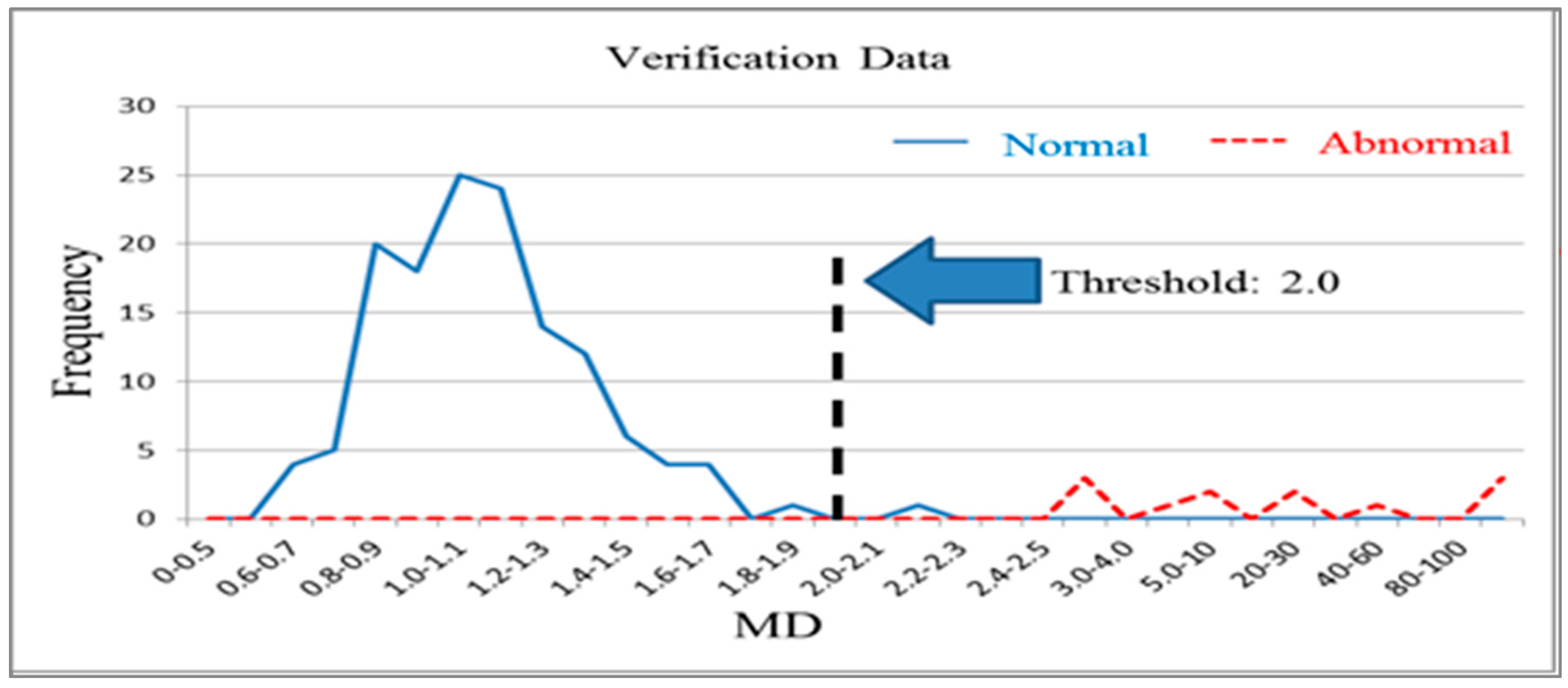
25]. These reduced models were used to calculate the Mahalanobis distances of the abnormal samples and obtain a single SN ratio. A greater SN ratio for the reduced model in comparison with that for the full model indicates that the system improved after performing MTS analysis. Therefore, the increases in SN ratio before and after analysis can be analyzed to assess improvements in system functioning. Finally, validation group data were used for testing to confirm whether the reduced model exhibited sufficient classification and diagnostic capabilities [
26,
27,
28,
29,
30].
2.3. Logistic Regression
Logistic regression model was introduced by Berkson [
31]. This model is used to resolve test result data with the possibility of only success or failure. The purpose of the model is to predict the relationship between a dependent variable and a set of independent variables accurately. The model also establishes a set of classification rules. Single samples can be entered to obtain a predicted probability of success. This probability is used to determine the properties of the sample. Logistic regression is used primarily in classification problems and is a statistical analysis method involving the use of class variables. The final predicted value for the dependent variable is a probability value between 0 and 1. Logistic regression is often used to establish binary classification as an alternative to linear discriminant analysis. This obviates the unreasonable assumption that covariance matrices used for binary classification are identical [
32]. Logistic regression is considered one of the most appropriate methods for predicting binary output [
33]. Logistic regression is currently more widely used with discrete binary data, particularly medical statistics and biostatistics. Scholars have also applied it to the fields of marketing and finance. Both logistic regression and discriminant analysis can resolve variable classification problems. However, logistic regression is not restricted by normal distribution assumptions. The basic form of logistic regression is identical to that of conventional linear regression. Dependent variable Y does not follow a normal distribution as the continuous variables required for linear regression do. Instead, it is a binary or dichotomous variable, such as success and failure or whether an event occurs. Thus, dependent variable estimates will always fall between 0 and 1.
Logistic regression uses a set of historical data with known attribution categories to derive a classification prediction model. This model is used to create classification criteria for new data. The primary goal of this model is to determine the relationships between the dependent and independent variables of the class types. The model can be used as a standard model for resolving the problem of dependent variables being binary data class variables, and can also be used to display function characteristics clearly. It is typically used within dependent variables to set the incident occurrence value to 1 (Y = 1) and the incident nonoccurrence value to 0 (Y = 0).
2.4. Neural Networks
The neural network algorithm uses mathematical language to describe the operating model of the human brain. These operating models are called neural networks. Neural networks are capable of learning. Users are not required to design complex programs to resolve problems. Neural networks have been applied widely to industrial control and business decisions, stock and exchange rate forecasting, voice recognition systems, and fault-tolerant systems. Kong [
34] applied neural networks to reduce the number of thin-film-transistor liquid-crystal display product test items during the manufacturing process, thereby reducing testing time and equipment investment. The results indicated that the application of neural networks reduced the original 102 test items to 32 items while maintaining high product testing accuracy. This demonstrates the effectiveness of neural networks, which are superior to conventional statistical regression methods [
35]. Hsieh [
36] applied neural networks to planning-based production in the paper industry. Hsieh used the superiority of neural networks in predicting demand. The networks learned the relationships among existing data to establish a demand forecasting model, which served as a basis for production planning for decision makers. Wang, Lin, Lai and Chen [
37] applied data mining techniques to increase the consistency of emergency triage. The study cooperated with the emergency department of a medical center in Taiwan to perform process construction, parameter selection, and sampling to construct a triage prediction model. This model generated 2000 pieces of necessary patient information. After conducting data mining using three classification techniques (multigroup discriminant analysis, multigroup logistic regression, and back-propagation neural networks), the study observed that back-propagation neural networks were able to distinguish patient criticality with 95.1% accuracy.
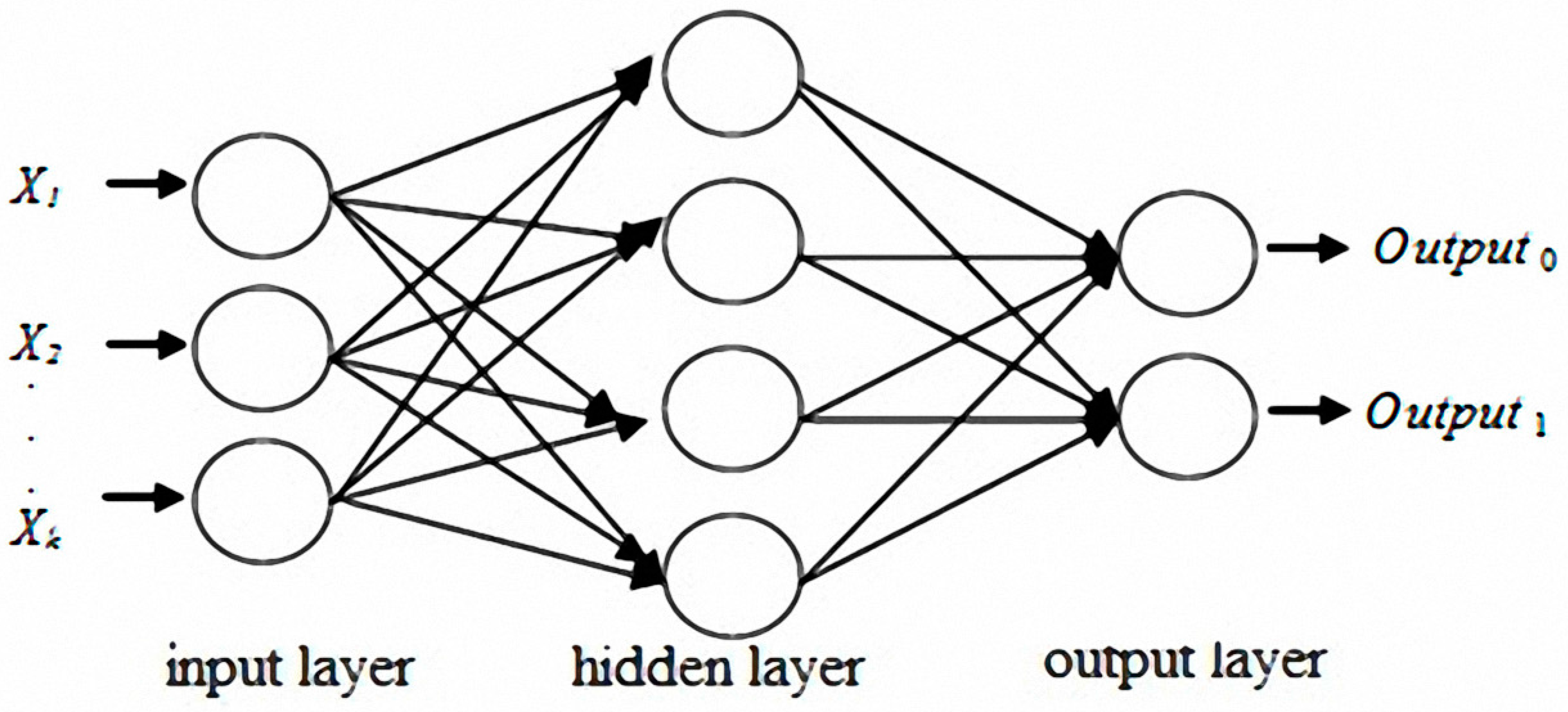
The original concept of neural networks was derived from biological nervous systems. Biological thinking is emulated using computers. Learning and thinking by using data generate answers for specific problems. A number of models have been presented for the development of neural networks. The most influential of these models is multilayer perceptron (MLP) [
38,
39,
40,
41]. MLP typically includes a number of layers, which are classified as input, hidden, or output layers. Each neuron in the input layer corresponds to a predictor variable, and the number of neurons is equal to the number of predictor variables. The number of neurons in the output layer is identical to the number of response variables [
42,
43].
Figure 3 shows that one or multiple hidden layers are possible.
The discussed studies revealed that the MTS, logistic regression and neural networks all demonstrated excellent discrimination when solving binary classification problems with multivariate data. The characteristic variable selections and classification prediction results obtained using the MTS are comparatively robust under identical data conditions. Therefore, the MTS architecture was analyzed, and logistic regression models and neural networks were used to improve the tablet PC product testing process. The differences among these three methods were subsequently compared and discussed.


 ,
, 