Trade-Offs between Economic and Environmental Optimization of the Forest Biomass Generation Supply Chain in Inner Mongolia, China


Abstract
1. Introduction
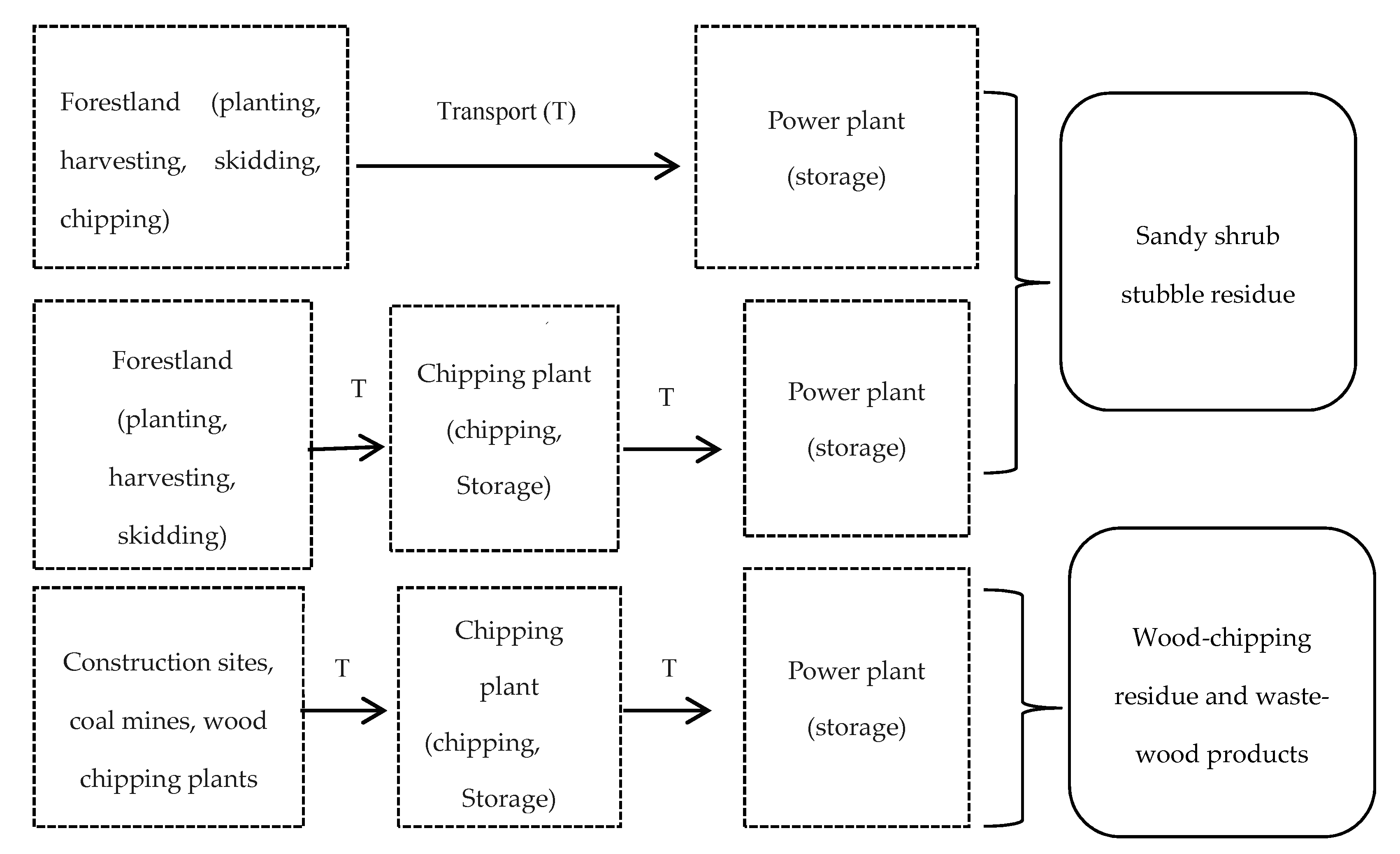
2. Materials and Methods
2.1. Model
2.1.1. Objective Function
2.1.2. Cost Functions
2.1.3. Carbon Dioxide Emissions Functions
2.1.4. Constraints
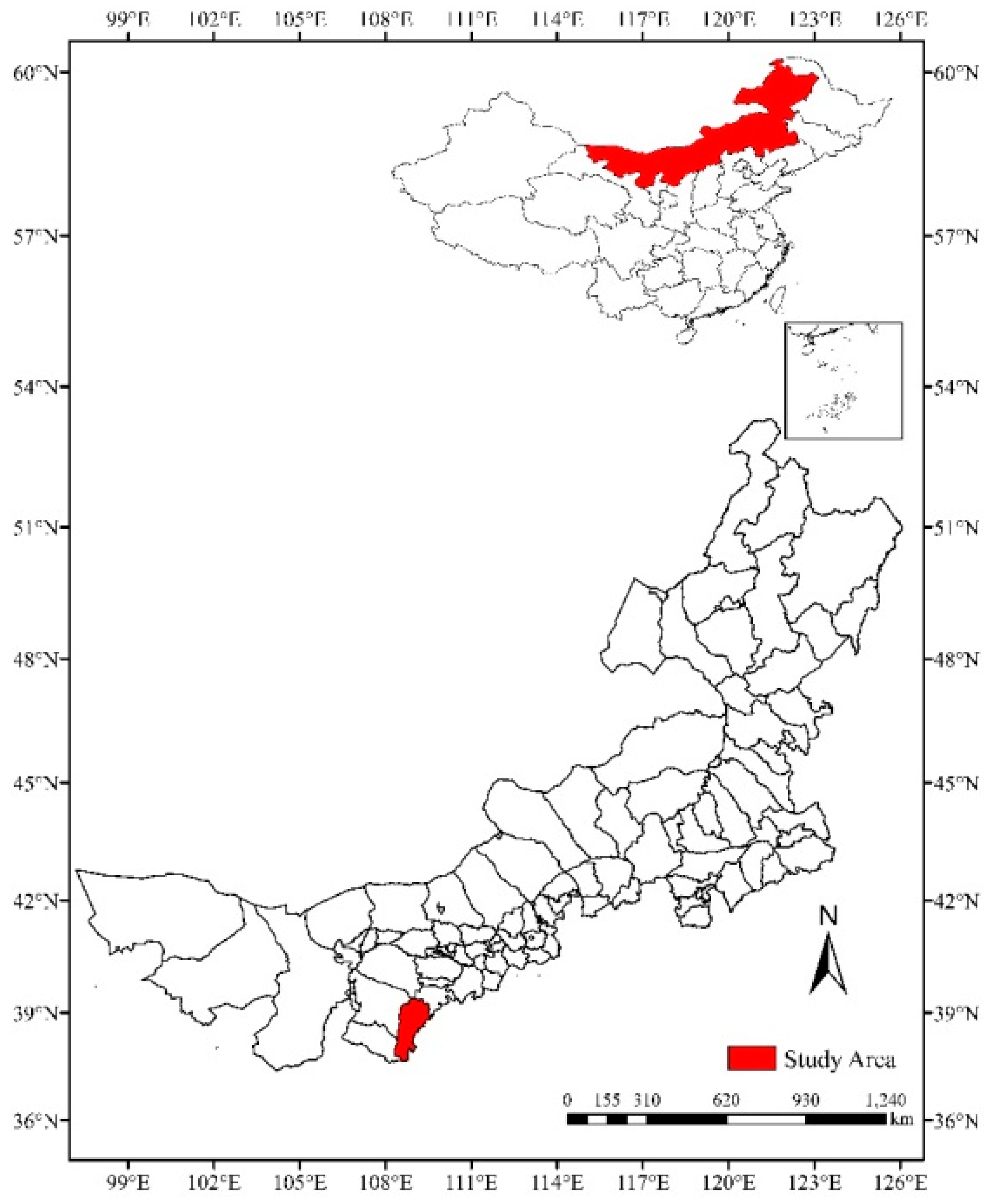
2.2. Data Source
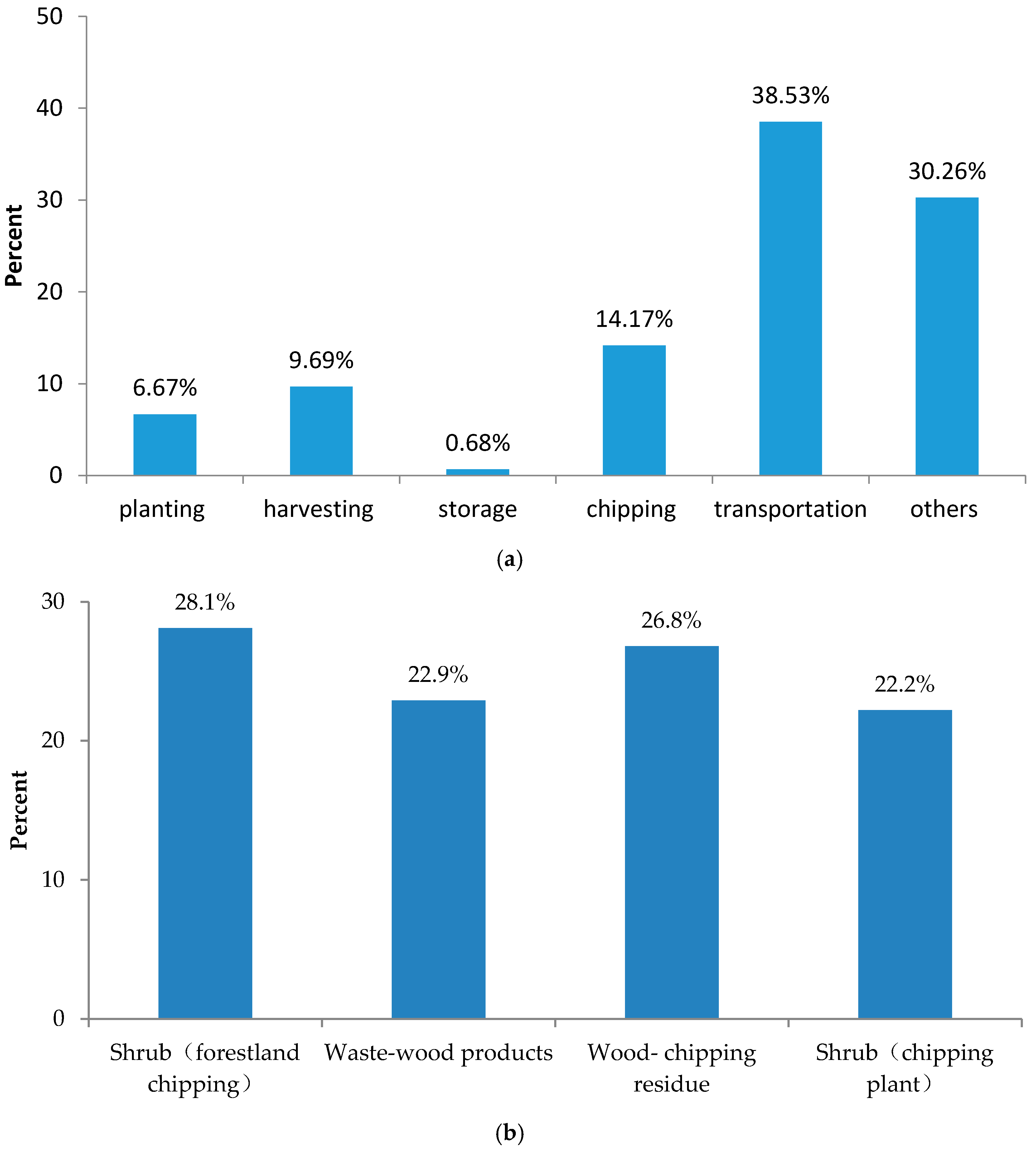
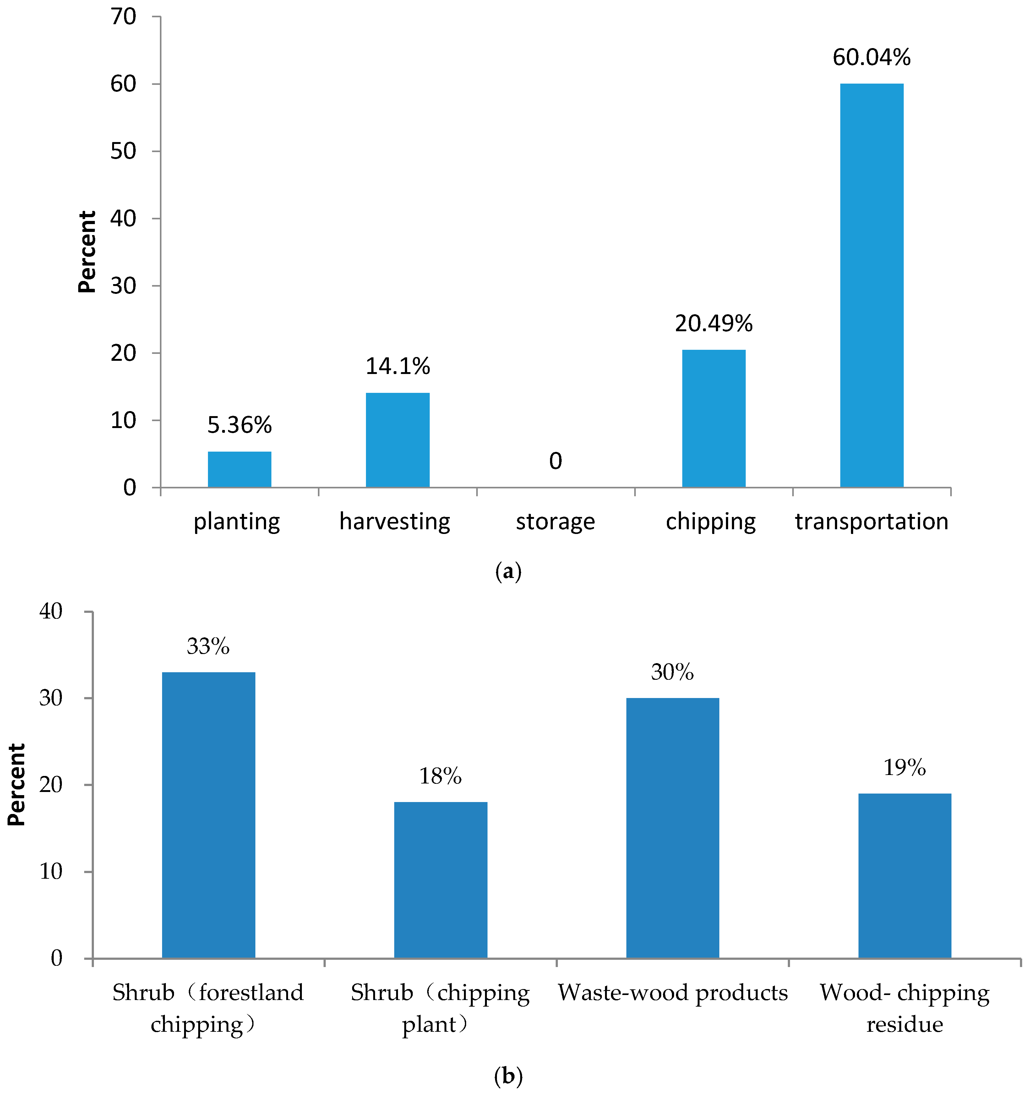
3. Results
4. Discussion
5. Conclusions
Acknowledgments
Author Contributions
Conflicts of Interest
Appendix A
| Name | Explanation |
| Raw material type | |
| Raw material transportation form | |
| Transportation path, | |
| Planting equipment, u | |
| Harvesting equipment v | |
| Skidding equipment, w | |
| Chipping equipment, x | |
| Transportation equipment, y | |
| Skidding point, | |
| Storage point, , | |
| Chipping point, |
References
- Lim, C.H.; Lam, H.L. Biomass supply chain optimisation via novel Biomass Element Life Cycle Analysis (BELCA). Appl. Energy 2016, 161, 733–745. [Google Scholar] [CrossRef]
- Srirangan, K.; Akawi, L.; Moo-Young, M.; Chou, C.P. Towards sustainable production of clean energy carriers from biomass resources. Appl. Energy 2012, 100, 172–186. [Google Scholar] [CrossRef]
- Lee, K.; Oh, W. Analysis of CO2 emissions in APEC countries: A time-series and a cross-sectional decomposition using the log mean Divisia method. Energy Policy 2006, 34, 2779–2787. [Google Scholar] [CrossRef]
- National Development and Reform Commission (NDRC). National Climate Change Plan for 2014–2020. 2011. Available online: http://www.sdpc.gov.cn/zcfb/zcfbtz/201201/t20120113_456506.html (accessed on 12 September 2017).
- Vinuya, F.; DiFurio, F.; Sandoval, E. A decomposition analysis of CO2 emissions in the United States. Appl. Econ. Lett. 2010, 17, 925–931. [Google Scholar] [CrossRef]
- China-nengyuan.com. Biomass Energy Development in 13th Five-Year Plan. 2016. Available online: http://www.china-nengyuan.com/news/101873.html (accessed on 12 September 2017).
- Zhang, L.; Zhang, C.H. Review of research on forest biomass energy development. Econ. Issues 2012, 10, 186–190. (In Chinese) [Google Scholar]
- Karjalainen, T.; Asikainen, A.; Ilavsky, J.; Zamboni, R.; Hotari, K.E.; Röser, D. Estimation of Energy Wood Potential in Europe; The Finnish Forest Research Institute: Vantaa, Finland, 2004; pp. 1–43. [Google Scholar]
- Smeets, E.M.W.; Faaij, A.P.C. Bioenergy potentials from forestry in 2050. Clim. Chang. 2006, 81, 353–390. [Google Scholar] [CrossRef]
- Zhang, C.H.; Zhang, L. Low-Carbon Economy and Forest Biomass Energy Development; China Forestry Press: Beijing, China, 2015; pp. 189–196. ISBN 978-750-387-929-6. (In Chinese) [Google Scholar]
- Allen, J.; Browne, M.; Hunter, A.; Boyd, J.; Palmer, H. Logistics management and costs of biomass fuel supply. Int. J. Phys. Distrib. Logist. Manag. 1998, 28, 463–477. [Google Scholar] [CrossRef]
- Development Status of Biomass Power Generation at Home and Abroad. 2015. Available online: https://wenku.baidu.com/view/3aef6db1ad02de80d5d84083 (accessed on 12 September 2017).
- Ranking Report on China’s Biomass Power Generation Enterprises in 2016. 2016. Available online: http://huanbao.bjx.com.cn/news/20170713/836917-2.shtml (accessed on 12 September 2017). (In Chinese).
- United Nations News. The Ecological Project of the Mao Wu Su Biomass Thermoelectric Company in Inner Mongolia, China Introduced Successful Experience in the United Nations. 2012. Available online: http://www.un.org/chinese/News/story.asp?NewsID=17465 (accessed on 12 September 2017).
- Shabani, N.; Akhtari, S.; Sowlati, T. Value chain optimization of forest biomass for bioenergy production: A review. Renew. Sustain. Energy Rev. 2013, 23, 299–311. [Google Scholar] [CrossRef]
- Cambero, C.; Sowlati, T.; Marinescu, M.; Röser, D. Strategic optimization of forest residue to bioenergy and biofuel supply chain. Int. J. Energy Res. 2015, 39, 439–452. [Google Scholar] [CrossRef]
- Klein, D.; Wolf, C.; Schulz, C.; Weber-Blaschke, G. Environmental impacts of various biomass supply chains for the provision of raw wood in Bavaria, Germany, with focus on climate change. Sci. Total Environ. 2016, 539, 45–60. [Google Scholar] [CrossRef] [PubMed]
- Roberts, D.G. Convergence of the fuel, food and fibre markets: A forest sector perspective. Int. For. Rev. 2008, 10, 81–94. [Google Scholar] [CrossRef]
- Trømborg, E.; Solberg, B. Forest sector impacts of the increased use of wood in energy production in Norway. For. Policy Econ. 2010, 12, 39–47. [Google Scholar] [CrossRef]
- Bolkesjo, T.F.; Tromborg, E.; Solberg, B. Bioenergy from the forest sector: Economic potential and interactions with timber and forest products markets in Norway. Scand. J. For. Res. 2006, 21, 175–185. [Google Scholar] [CrossRef]
- Raunikar, R.; Buongiorno, J.; Turner, J.A.; Zhu, S. Global outlook for wood and forests with the bioenergy demand implied by scenarios of the Intergovernmental Panel on Climate Change. For. Policy Econ. 2010, 12, 48–56. [Google Scholar] [CrossRef]
- Sjølie, H.K.; Trømborg, E.; Solberg, B.; Bolkesjø, T.F. Effects and costs of policies to increase bioenergy use and reduce GHG emissions from heating in Norway. For. Policy Econ. 2010, 12, 57–66. [Google Scholar] [CrossRef]
- Schwarzbauer, P.; Stern, T. Energy vs. material: Economic impacts of a “wood-for-energy scenario” on the forest-based sector in Austria—A simulation approach. For. Policy Econ. 2010, 12, 31–38. [Google Scholar] [CrossRef]
- Bürger, V.; Klinski, S.; Lehr, U.; Leprich, U.; Nast, M.; Ragwitz, M. Policies to support renewable energies in the heat market. Energy Policy 2008, 36, 3150–3159. [Google Scholar] [CrossRef]
- Zhang, Y. The Policy Research on Renewable Energy Price in the Inner Mongolia. Master’s Thesis, Inner Mongolia University, Hohhot City, China, 2015. (In Chinese). [Google Scholar]
- Xie, L.L. Analysis on Supporting Policy of Forestry Biomass Energy Industry in China. Master’s Thesis, Beijing Forestry University, Beijing, China, 2014. (In Chinese). [Google Scholar]
- Sun, F.L.; Wang, Z.Y.; Ye, H. Development Status, Possible Impacts and Countermeasures of Forest biomass Industry. Econ. Issues 2012, 3, 149–153. (In Chinese) [Google Scholar]
- Dong, F.X. Study on the Development of Wood Biomass Energy in China Based on Regional Forest Resources. Master’s Thesis, Beijing Forestry University, Beijing, China, 2014. (In Chinese). [Google Scholar]
- Oberscheider, M.; Zazgornik, J.; Henriksen, C.B.; Gronalt, M.; Hirsch, P. Minimizing driving times and greenhouse gas emissions in timber transport with a near-exact solution approach. Scand. J. For. Res. 2013, 28, 493–506. [Google Scholar] [CrossRef]
- Whalley, S.; Klein, S.J.W.; Benjamin, J. Economic analysis of woody biomass supply chain in Maine. Biomass Bioenergy 2017, 96, 38–49. [Google Scholar] [CrossRef]
- Yoshioka, T.; Aruga, K.; Nitami, T.; Sakai, H.; Kobayashi, H. A case study on the costs and the fuel consumption of harvesting, transporting, and chipping chains for logging residue in Japan. Biomass Bioenergy 2006, 30, 342–348. [Google Scholar] [CrossRef]
- Gunnarsson, H.; Rönnqvist, M.; Lundgren, J.T. Supply chain modelling of forest fuel. Eur. J. Oper. Res. 2004, 158, 103–123. [Google Scholar] [CrossRef]
- Rentizelas, A.A.; Tolis, A.J.; Tatsiopoulos, I.P. Logistics issues of biomass: The storage problem and the multi-biomass supply chain. Renew. Sustain. Energy Rev. 2009, 13, 887–894. [Google Scholar] [CrossRef]
- Emer, B.; Grigolato, S.; Lubello, D.; Cavalli, R. Comparison of biomass feedstock supply and demand in Northeast Italy. Biomass Bioenergy 2011, 35, 3309–3317. [Google Scholar] [CrossRef]
- Serengil, Y.; Pamukçu, P. Managing Forests as Complex Adaptive Systems—Building Resilience to the Challenge of Global Change. Int. J. Environ. Stud. 2013, 71, 117–119. [Google Scholar] [CrossRef]
- Shabani, N.; Sowlati, T. A mixed integer non-linear programming model for tactical value chain optimization of a wood biomass power plant. Appl. Energy 2013, 104, 353–361. [Google Scholar] [CrossRef]
- Zhou, Y.; Xu, S.Y.; Qian, X.H.; Han, Z.Z.; Wang, K.F. Study on multi-objective optimization model of bio-energy production. Comput. Appl. Chem. 2007, 24, 1501–1504. (In Chinese) [Google Scholar]
- Zhou, Y.; Li, D.; Wu, Z.L.; Zhou, C.J.; Zheng, L.F. Study on carbon emissions in the forest transporting operation. For. Eng. 2014, 30, 1–5. (In Chinese) [Google Scholar]
- Zheng, W.W.; Zhang, L.Y.; Qiu, R.Z. Study on Carbon Emissions from Woody Biomass Raw Material Supply Chain in Fujian Province. J. Southwest For. Univ. 2015, 35, 77–82. (In Chinese) [Google Scholar]
- Zheng, W.W. The Optimization of Raw Material for Wood-Biomass Energy Plant Supply Chain Based on the LCA. Master’s Thesis, Fujian Agriculture and Forestry University, Fuzhou, China, 2016. (In Chinese). [Google Scholar]
- Zhang, D.H.; Mi, F.; Wu, W.H. Technical Economics; China Forestry Press: Beijing, China, 2012; pp. 123–156. ISBN 978-750-386-800-9. (In Chinese) [Google Scholar]
- National Bureau of Statistics of the People’s Republic of China. China Statistical Yearbook 2016. 2016. Available online: http://www.stats.gov.cn/tjsj/ndsj/2016/indexch.htm (accessed on 12 September 2017).
- National Bureau of Statistics of the People’s Republic of China. China Energy Statistical Yearbook 2014. 2015. Available online: http://www.stats.gov.cn/tjsj./tjcbw/201512/t20151210_1287828.html (accessed on 12 September 2017).
- China’s Forestry. Inner Mongolia Autonomous Region Forestry Department Website News. 2015. Available online: http://www.nmglyt.gov.cn/cyc/cyxx/ltqy/201508/t20150824_113300.html (accessed on 12 September 2017).
- Valente, C.; Hillring, B.G.; Solberg, B. Bioenergy from mountain forest: A life cycle assessment of the Norwegian woody biomass supply chain. Scand. J. For. Res. 2011, 26, 429–436. [Google Scholar] [CrossRef]
- Blouin, M.; Cormier, D. Carbon and Greenhouse Gas Accounting of Forest Operations in FPInterface. Int. J. For. Eng. 2012, 23, 64–69. [Google Scholar] [CrossRef]


| Energy | Unit Price | Density | Average Low Calorific Value (kJ∙kg−1) | Carbon Emissions Coefficient |
|---|---|---|---|---|
| ($∙L−1) | (kg∙L−1) | (kg∙L−1) | ||
| Gasoline | 6.41 | 0.728 | 43,070 | 2.925 |
| Diesel | 5.94 | 0.84 | 42,652 | 3.095 |
| Equipment Parameters | Forestland | Chipping Plant | Unit |
|---|---|---|---|
| Purchase cost | 2.75 | 29.77 a | thousand $ |
| Service life | 8 | 5 | year |
| Annual maintenance costs | 0.37 | 0.74 | thousand $ |
| Power | 53 × 103 | 120 × 103 | w |
| Energy consumption per h | 1.47 | 2.41 | L |
| Carbon emissions factor | 3.82 | 7.91 | kg∙h−1 |
| Labor input per day | 1.50 | 15 | worker |
| Labor price per day | 0.02 | 0.01 | thousand $ |
| Amount of raw materials processed per h | 0.63 | 25 | thousand kg |
| Parameters | Value |
|---|---|
| Maximum unit load of agricultural tricycle | 1.5 × 10³ kg |
| Agricultural tricycle fuel consumption 100 km | 8 L |
| Carbon emissions factor of agricultural tricycle | 0.171 kg∙km−1 |
| Maximum unit load of truck | 10 × 103 kg |
| Trucks fuel consumption of 100 km | 38.5 L |
| Carbon emissions factor of truck | 0.481 kg∙km−1 |
| Three Key Raw Materials | Current Supply Amount | Optimization Supply Amount | Differences |
|---|---|---|---|
| Sandy shrub stubble residue | 90,000 | 93,750 | 3750 |
| Wood-chipping residue | 40,000 | 40,000 | 0 |
| Waste-wood products | 50,000 | 46,250 | −3750 |
| Total | 180,000 | 180,000 | 0 |
| Supply Cost | Shrub (Forest Land) | Shrub (Chipping Plant) | Wood-Chipping Residue | Waste-Wood Products | Total Cost of Each Node | Differences between the Total Cost of Each Node in Two Situations (b − a) | |
|---|---|---|---|---|---|---|---|
| Planting | a | 355.8 | 148.9 | 0 | 0 | 504.7 | −8.2 |
| b | 317.8 | 178.7 | 0 | 0 | 496.5 | ||
| Harvesting | a | 479.3 | 259.1 | 0 | 0 | 738.4 | −16.2 |
| b | 462.2 | 260 | 0 | 0 | 722.2 | ||
| Storage | a | 7 | 15 | 13.5 | 16.9 | 52.5 | −1.3 |
| b | 6.8 | 15.2 | 13.5 | 15.6 | 51.2 | ||
| Chipping | a | 648.7 | 165.8 | 0 | 276.3 | 1090.8 | −35.4 |
| b | 613.3 | 186.5 | 0 | 255.6 | 1055.4 | ||
| Transportation | a | 745 | 575.7 | 705.1 | 881.4 | 2907.1 | −36.2 |
| b | 695 | 647.6 | 705.1 | 881.4 | 2871 | ||
| Others | a | 0 | 288.7 | 989.7 | 977.4 | 2255.9 | −1.1 |
| b | 0 | 360.9 | 989.7 | 904.1 | 2254.8 | ||
| Total cost of raw materials | a | 2235.8 | 1453.2 | 1708.4 | 2152 | 7549.4 | −98.4 |
| b | 2095 | 1649 | 1708.4 | 1998.6 | 7451 | ||
| Differences between total cost of raw materials in two situations (b − a) | −140.8 | 195.8 | 0 | −153.4 | −98.4 | -- | |
| The unit cost per thousand kg of raw materials | a | 0.037 | 0.048 | 0.043 | 0.043 | -- -- | |
| b | 0.035 | 0.049 | 0.043 | 0.043 | -- -- | ||
| Differences between the unit cost per thousand kg of raw materials in two situations (b − a) | −0.0023 | 0.0009 | 0 | 0.0002 | -- | -- | |
| CO2 Emissions | Shrub (Forest Land) | Shrub (Chipping Plant) | Wood-Chipping Residue | Waste-Wood Products | Total Emissions of Each Node | Differences between Total Emissions of Each Node in Two Situations (b − a) | |
|---|---|---|---|---|---|---|---|
| Planting | a | 195.1 | 109.8 | 0 | 0 | 304.9 | −0.1 |
| b | 195.1 | 109.7 | 0 | 0 | 304.8 | ||
| Harvesting | a | 594.6 | 207.8 | 0 | 0 | 802.4 | −0.7 |
| b | 594.5 | 207.2 | 0 | 0 | 801.8 | ||
| Storage | a | 0.002 | 0.000 | 0.001 | 0.001 | 0.0 | 0.0 |
| b | 0.002 | 0.005 | 0.005 | 0.001 | 0.0 | ||
| Chipping | a | 410.6 | 313.9 | 0 | 465 | 1189.5 | −24.9 |
| b | 420.6 | 313.9 | 0 | 430.1 | 1164.6 | ||
| Transportation | a | 689.5 | 392.8 | 1075.2 | 1300 | 3457.5 | −44.8 |
| b | 689.7 | 382.4 | 1075.2 | 1265.4 | 3412.7 | ||
| Total emissions of raw materials | a | 1889.8 | 1014.3 | 1075.2 | 1765.0 | 5744.4 | −60.6 |
| b | 1899.8 | 1013.3 | 1075.2 | 1695.5 | 5683.8 | ||
| Differences between total emissions of materials in two situations(b − a) | 10.0 | −1.1 | 0 | −69.5 | −60.6 | -- | |
| The unit emissions per thousand kg of raw materials | a | 0.0315 | 0.0338 | 0.0269 | 0.0353 | -- | |
| b | 0.0317 | 0.0300 | 0.0269 | 0.0367 | -- -- | ||
| Differences between the unit emissions per thousand kg of raw materials in two situations (b − a) | 0.0002 | −0.0038 | 0 | 0.0014 | -- | -- | |
| Rate | Transportation Distance (km) | Supply Cost (Thousand $) | CO2 Emissions (Thousand kg) |
|---|---|---|---|
| −30% | 84.13 | 7333.7 | 5356.9 |
| −20% | 95.77 | 7372.1 | 5463.9 |
| −10% | 107.74 | 7411.5 | 5573.8 |
| 0% | 119.71 | 7450.9 | 5683.8 |
| 10% | 131.68 | 7490.4 | 5793.7 |
| 20% | 143.66 | 7529.8 | 5903.7 |
| 30% | 155.60 | 7569.2 | 6304.7 |
| Rate | Unit Chipping Cost (Thousand $) | Supply Cost (Thousand $) | CO2 Emissions (Thousand kg) |
|---|---|---|---|
| −14.7% | 0.00872 | 7180.7 | 5729.2 |
| −10% | 0.00920 | 7267.2 | 5712.2 |
| 0.0% | 0.01022 | 7450.9 | 5683.8 |
| 10% | 0.01124 | 7634.6 | 5692.8 |
| 14.7% | 0.01172 | 7721.2 | 5698.2 |
© 2017 by the authors. Licensee MDPI, Basel, Switzerland. This article is an open access article distributed under the terms and conditions of the Creative Commons Attribution (CC BY) license (http://creativecommons.org/licenses/by/4.0/).
Share and Cite
Zhang, M.; Wang, G.; Gao, Y.; Wang, Z.; Mi, F. Trade-Offs between Economic and Environmental Optimization of the Forest Biomass Generation Supply Chain in Inner Mongolia, China. Sustainability 2017, 9, 2030. https://doi.org/10.3390/su9112030
Zhang M, Wang G, Gao Y, Wang Z, Mi F. Trade-Offs between Economic and Environmental Optimization of the Forest Biomass Generation Supply Chain in Inner Mongolia, China. Sustainability. 2017; 9(11):2030. https://doi.org/10.3390/su9112030
Chicago/Turabian StyleZhang, Min, Guangyu Wang, Yi Gao, Zhenqi Wang, and Feng Mi. 2017. "Trade-Offs between Economic and Environmental Optimization of the Forest Biomass Generation Supply Chain in Inner Mongolia, China" Sustainability 9, no. 11: 2030. https://doi.org/10.3390/su9112030
APA StyleZhang, M., Wang, G., Gao, Y., Wang, Z., & Mi, F. (2017). Trade-Offs between Economic and Environmental Optimization of the Forest Biomass Generation Supply Chain in Inner Mongolia, China. Sustainability, 9(11), 2030. https://doi.org/10.3390/su9112030