Natural Resource Economics, Planetary Boundaries and Strong Sustainability

Abstract

Earth systems science maintains that there are nine “planetary boundaries” that demarcate a sustainable, safe operating space for humankind for essential global sinks and resources. Respecting these planetary boundaries represents the “strong sustainability” perspective in economics, which argues that some natural capital may not be substituted and are inviolate. In addition, the safe operating space defined by these boundaries can be considered a depletable stock. We show that standard tools of natural resource economics for an exhaustible resource can thus be applied, which has implications for optimal use, price paths, technological innovation, and stock externalities. These consequences in turn affect the choice of policies that may be adopted to manage and allocate the safe operating space available for humankind.

1. Introduction

There is a growing scientific literature emphasizing that human populations and economic activity are rapidly approaching and even exceeding the limits of key sub-systems and processes of the global environment, which could lead to abrupt phase changes, or “tipping points” in the Earth system [1,2,3,4,5,6]. This literature has identified “nine such processes for which we believe it is necessary to define planetary boundaries: climate change; rate of biodiversity loss (terrestrial and marine); interference with the nitrogen and phosphorus cycles; stratospheric ozone depletion; ocean acidification; global freshwater use; change in land use; chemical pollution; and atmospheric aerosol loading.” [2] (p. 472).

For example, terrestrial net primary (plant) production could provide a measurable boundary for human consumption of Earth’s biological resources [3]. Freshwater supplies and ecosystems need to be protected by a limit on global and basin-wide consumptive uses of water [4,5]. A planetary boundary for biodiversity loss could be based on extinction rates but also measures of functional and genetic diversity as well as biome conditions [4,6]. Limits on land-system change could be set in terms of forested land as a percentage of original forest cover or potential forest [4]. Finally, the global carbon budget is the cumulative amount of anthropogenic CO₂ emissions that would prevent global warming from exceeding 2 °C [7].

The purpose of establishing these planetary boundaries is to demarcate a “safe operating space for humanity” [2] (p. 472). The safe operating space places an absolute limit on how much economic activity can safely exploit critical global biophysical subsystems or processes. To date, the focus has been on characterizing and quantifying the various planetary boundaries rather than suggesting “how to maneuver within the safe operating space in the quest for global sustainability” [4] (p. 744). Yet, if planetary boundaries limit some uses of the global environment, it is essential to develop models that inform stewardship of this “safe operating space” [8]. Here, we outline the key features of such a modeling approach, and explore its implications for policy.

First, we suggest that respecting planetary boundaries conforms to the “strong sustainability” perspective in economics, which argues that some natural capital may not be substituted and are inviolate [9]. In addition, the safe operating space defined by these boundaries can be considered a depletable stock. Our analysis therefore has implications for optimal use, price paths, innovation and the valuation of “stock externalities”. These implications in turn affect the choice of policies that may be adopted to manage and allocate the safe operating space available for humankind.

2. Materials and Methods

2.1. Key Definitions and Concepts

We first establish the link between, on the one hand, the concepts of planetary boundaries and safe operating space in the Earth system science literature, and on the other, the concepts of weak and strong sustainability in economics.

The key rationale for establishing planetary boundaries on anthropogenic processes is to avoid “tipping points” or “thresholds” that could lead to irrevocable changes in this system, with potentially catastrophic impacts for humanity. As noted in the Introduction, scientists have identified nine processes resulting from human activity that should be subject to planetary boundaries [1,2,3,4,5,6]:

• Climate change
• Loss of biosphere integrity (e.g., marine and terrestrial biodiversity loss)
• Land-system change
• Freshwater use
• Biochemical flows (e.g., effluents that interfere with nitrogen and phosphorous cycles)
• Ocean acidification
• Atmospheric aerosol loading
• Stratospheric ozone depletion
• Novel entities (e.g., new substances and modified organisms that have undesirable environmental impacts).

If unchecked, these processes could place human population growth and economic activity on an unsustainable trajectory that crosses critical thresholds and de-stabilizes the global environment. Establishing planetary boundaries therefore “aims to help guide human societies away from such a trajectory by defining a ‘safe operating space’ in which we can continue to develop and thrive” [4] (p. 737). In addition, the boundary defining the safe operating space should include a “buffer” that both accounts for “uncertainty in the precise position of the threshold” and “also allows society time to react to early warning signs that it may be approaching a threshold and consequent abrupt or risky change” [4] (pp. 737–738). Figure 1 illustrates how setting a planetary boundary to designate the safe operating space is impacted by the uncertainty and lack of information over possible future threshold effects.

The concept of a planetary boundary that imposes an absolute limit on human activities that threaten critical Earth system resources and sinks is directly relevant to the capital approach to sustainability [9,10,11]. This approach suggests that economic wealth comprises three distinct assets: manufactured, or reproducible capital (e.g., roads, buildings, machinery, factories, etc.); human capital, which are the skills, education and health embodied in the workforce; and natural capital, including land, forests, fossil fuels, minerals, fisheries and all other natural resources, regardless of whether or not they are exchanged on markets or owned. In addition, natural capital also consists of those ecosystems that through their natural functioning and habitats provide important goods and services to the economy. For example, [12] (p. 395) state, “the world’s ecosystems are capital assets. If properly managed, they yield a flow of vital services, including the production of goods (such as seafood and timber), life support processes (such as pollination and water purification), and life-fulfilling conditions (such as beauty and serenity).”

The capital approach to sustainability asserts that the value of the aggregate stock of all capital—reproducible, human and natural—must be maintained or enhanced over time to ensure that overall welfare does not decline. However, within this approach, there are contrasting weak versus strong sustainability views, which differ in the treatment of natural capital (see

Table 1. Weak versus Strong Sustainability.

Weak Sustainability	Strong Sustainability
Natural, human and reproducible capital can be substituted for each other. Natural, human and reproducible capital are an aggregate, homogeneous stock.	Cannot always substitute for natural capital with reproducible or human capital. Cannot view natural, reproducible and human capital as a homogeneous stock.
Natural capital should be used efficiently over time. As long as depleted natural capital is replaced with even more valuable reproducible and human capital, then the value of the aggregate stock will increase.	Certain environmental sinks, processes and services are unique and essential, subject to irreversible loss, and there is uncertainty over their future value and importance.
Maintaining and enhancing the value of this aggregate capital stock is sufficient for sustainability.	Maintaining and enhancing the value of the value of the aggregate capital stock is necessary but not sufficient. Sustainability also requires preserving unique and essential natural capital.

). As pointed out by [9] (p. 42), “the main disagreement is whether natural capital has a unique or essential role in sustaining human welfare, and thus whether special ‘compensation rules’ are required to ensure that future generations are not made worse off by natural capital depletion today”. Weak sustainability assumes that there is no difference between natural and other forms of capital (e.g., human or reproducible), and thus as long as depleted natural capital is replaced with more value human or reproducible capital, then the total value of wealth available to current and future generations will increase. In contrast, strong sustainability argues that some natural capital is essential (e.g., unique environments, ecosystems, biodiversity and life-support functions), subject to irreversible loss, and has uncertain value. Consequently, the sustainability goal of maintaining and enhancing the value of the aggregate capital stock requires preserving essential natural capital.

Thus, scientists [1,2,3,4,5,6] who advocate the need for planetary boundaries to limit human impacts on critical global sinks and resources are aligning with the strong sustainability perspective, which argues that some natural capital may not be substituted and are inviolate. Based on this scientific view, some economists have begun examining how such planetary boundaries should be established, given the uncertainty over thresholds, abrupt and irreversible change, and the magnitude of welfare impacts [8,13].

Equally important, however, is determining how to manage efficiently and sustainable the safe operating space available for exploitation by humankind [4,8]. For this purpose, the weak sustainability perspective is relevant. Here, we show how such a perspective can be adopted to develop a model that informs “wise stewardship” of any safe operating space defined by planetary boundaries.

Specifically, we consider the safe operating space defined by any planetary boundary to be a depletable stock that has value either as a source of natural resource inputs into an economy or a sink for emitted waste. The safe operating space can therefore be treated as an economic asset that should earn a rate return comparable to holding other assets in an economy. Following the principles of weak sustainability (Table 1), sustainable management of this asset requires efficient use over time. This has consequences that, in turn, affect the choice of policies that may be adopted to manage and allocate the safe operating space available for humankind.

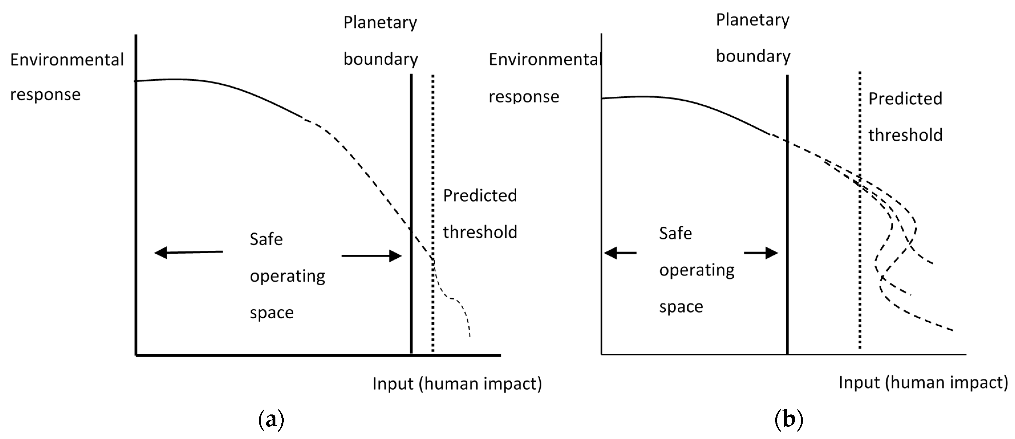
2.2. The Safe Operating Space as an Economic Asset

The starting point for our modeling approach is to treat the safe operating space defined by planetary boundaries as an economic asset.

Let the initial safe operating space associated with a given planetary boundary be denoted as S₀. Depending on the planetary boundary, this measurable limit could be terrestrial net primary production, available freshwater for consumption, species richness, assimilative capacity for various pollutants, forest land area, or the global carbon budget [1,2,3,4,5,6]. No matter how it is delineated and measured, S₀ is a finite, depletable stock that can be safely used, exploited or converted through economic activity. Consequently, the initial safe operating space can be considered an economic asset.

At time t, some of the initial S₀ will already have been “used up” by the economy. Define $C\left(t\right)={\displaystyle {\int }_0^{t}c\left(s\right)ds}$ as the cumulative amount of the safe operating space that has already been depleted by economic activity. The remaining stock of this asset at time t is therefore $S\left(t\right)$, and it follows that

$${\displaystyle {\int }_0^{t}c\left(s\right)}ds=S_0-S\left(t\right), \dot{S}=-c\left(t\right),$$

(1)

where a dot over a variable indicates its derivative with respect to t.

As the safe operating space is an economic asset, its cumulative exploitation must earn a rate of return that is comparable to all other forms of capital available to the economy. Let the average rate of return across all the latter assets be denoted as some interest rate r. Also, assume that cumulative exploitation of the safe operating space up to time t is for various market-oriented activities, which have market prices that can be aggregated into some average price index $p\left(t\right)$. For analytical convenience, we assume that the market price is net of any cost of exploitation. Thus, cumulative exploitation is sold at this market price and the proceeds $p\left(t\right)\left(S_0-S\left(t\right)\right)$ are invested at interest rate r.

Depending on the type of planetary boundary, the available safe operating space at time t might increase, due to natural (i.e., biological) growth or recovery of assimilative capacity. This is especially true for any $S\left(t\right)$ that is defined in terms of biological or land resources, such as forest land or species stocks. But it might also hold true for sinks of carbon, ocean recovery from acidification, nitrogen and phosphorus cycles, replenishment of freshwater ecosystems, and so on. Representing such natural growth or recovery as $F\left(S\left(t\right)\right),\hspace{0.17em}{F}^{\prime }>0$, we assume that any such additional augmentation of the available safe operating space at time t will be immediately exploited at the rate $x\left(t\right)=F\left(S\left(t\right)\right)$, and also sold at the same market price $p\left(t\right)$ for cumulative exploitation.

There are two additional values of the safe operating space that should be considered. First, the remaining natural asset $S\left(t\right)$ may realize capital gains or losses if market prices change. These gains or losses at any time t are $\dot{p}S\left(t\right)$. Second, the available safe operating space, especially if it includes maintenance of important habitats, ecosystems or biological species, may generate wider social benefits, or “stock externalities”, such as biodiversity values, watershed protection, carbon sequestration and ecotourism. We assume that, for any remaining $S\left(t\right)$, the aggregate value of stock externalities is $V\left(t\right)$, which can be expressed in turn as a “markup” v of the market price of exploiting the safe operating space. The rationale for such a markup is straightforward: If the social value of any stock externalities is less than or equal to the market price of exploiting the safe operating space, then S(t) would not be conserved. Thus, the social benefit associated with any such stock externalities is $V(t)S\left(t\right)=vp\left(t\right)S\left(t\right)$.

Consequently, optimal management of the safe operating space at time t requires choosing the amount of remaining $S\left(t\right)$ that maximizes all the above values associated with this asset, i.e.,

$$\underset{S\left(t\right)}{Max}W\left(t\right)=rp\left(t\right)\left(S_0-S\left(t\right)\right)+p\left(t\right)F\left(S\left(t\right)\right)+\dot{p}S\left(t\right)+vp\left(t\right)S\left(t\right).$$

(2)

Suppressing the time argument for analytical convenience, the first-order condition yields

$$\frac{\dot{p}}{p}+F^{\prime }+v=r,$$

(3)

which is the optimal portfolio balance equation for $S\left(t\right)$. The left-hand side represents the marginal returns for holding on to the remaining safe operating space rather than exploiting it. The right-hand side is the opportunity cost, in terms of foregone interest income from other economic assets, from retaining $S\left(t\right)$. Note that $r-\dot{p}/p\ge F^{\prime }+v\to S\left(t\right)=0$, which implies that the remaining safe operating space is at risk if $r-\dot{p}/p$ is large, or $F^{\prime }$ and v are small. Also, if natural growth or recovery and stock externalities are negligible, then (3) resembles the more familiar Hotelling efficiency condition associated with a pure exhaustible resource, i.e., $\dot{p}/p=r$.

For analytical convenience, we assume that the marginal rate of biological growth of recovery is constant, so that we can denote $F^{\prime }\left(S\left(t\right)\right)=f$. This allows Equation (3) to be rewritten as $\dot{p}-\left(r-v-f\right)p=0$, which yields the following solution for the price path

$$p\left(t\right)=p_0{e}^{\mathsf{\rho }t},\hspace{0.17em}\hspace{0.17em}\hspace{0.17em}\mathsf{\rho }=r-v-f.$$

(4)

The market price associated with exploiting the safe operating space should evolve at a rate equal to the net rate of return ρ earned from investing the proceeds from such exploitation. This price path is increasing if $r>v+f$, suggesting that there are positive net returns from exploiting and investing the proceeds. Consequently, it pays to exploit the safe operating space today, there will be less available for exploitation in future periods, and so p must rise over time. Alternatively, as $\mathsf{\rho }\to 0$, then there are no net returns to the invested proceeds earned from exploiting $S\left(t\right)$, and the safe operating space will be conserved indefinitely.

3. Results

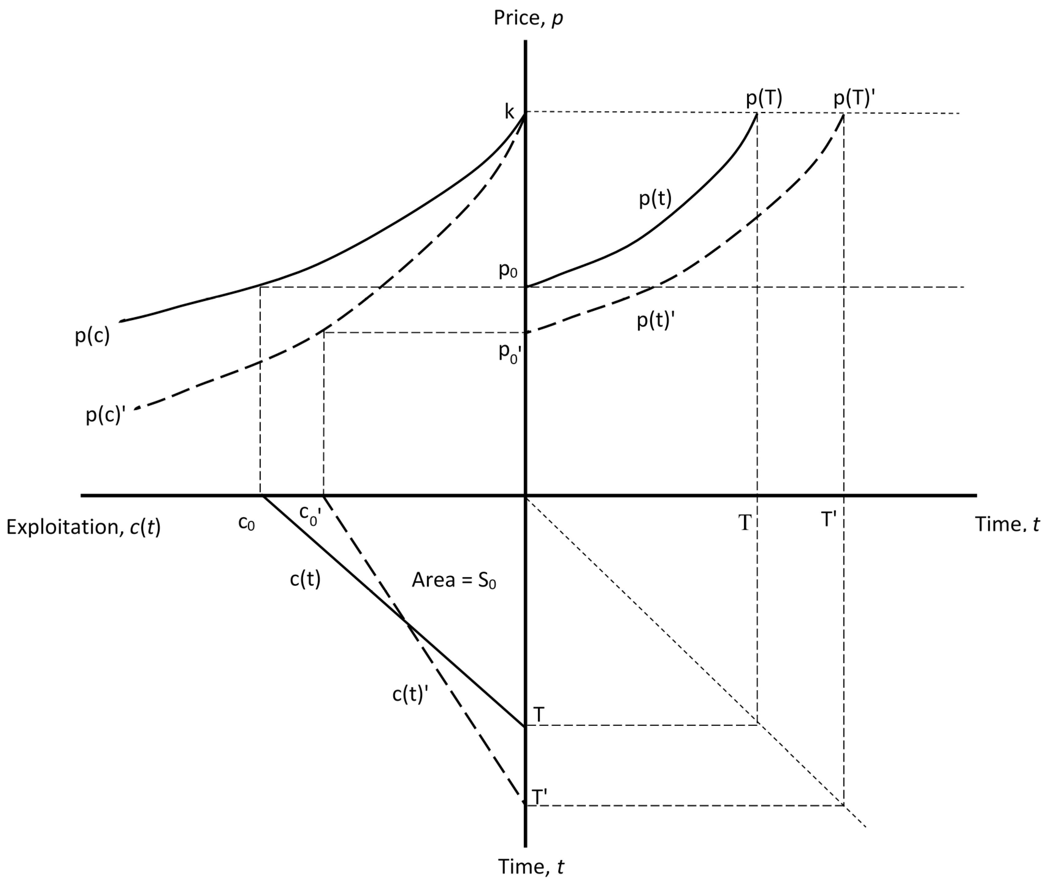
3.1. Optimal Exploitation of the Safe Operating Space

The above efficiency conditions Equations (3) and (4) for managing the safe operating space as an economic asset also allow determination of the optimal exploitation of the remaining stock $S\left(t\right)$.

We assume that such exploitation occurs over a finite time period $\left[0,T\right]$, and that any time t there is an inverse demand function for the marketed products $p=p\left(c\left(t\right)\right)$. The net social benefit from exploitation is therefore $B\left(c\left(t\right)\right)={\displaystyle \underset{0}{\overset{c\left(t\right)}{\int }}p\left(s\right)ds}$. If follows that we can specify the discounted social welfare over the entire planning horizon as

$$U={\displaystyle {\int }_0^{T}B\left(c\left(t\right)\right)e^{-\mathsf{\rho }t}}dt, B\left(c\left(t\right)\right)={\displaystyle \underset{0}{\overset{c\left(t\right)}{\int }}p\left(s\right)ds}, \frac{\partial B}{\partial c}=p\left(c\right).$$

(5)

Note that in Equation (5) the discount rate for social welfare is the net rate of return earned from investing the proceeds of exploitation ρ derived previously. This allows optimal exploitation of the safe operating space $c\left(t\right)$ to satisfy the optimal portfolio balance condition Equation (3) associated with managing $S\left(t\right)$ as an economic asset. Moreover, it also means that the net price of exploitation must equal the marginal value associated with conserving the safe operating space.

To see this, let $\mathsf{\lambda }\left(t\right)$ be the shadow value in terms of social welfare of having an additional unit of $S\left(t\right)$, which by definition is $\partial U/\partial S$. Two necessary conditions for maximizing social welfare Equation (5) with respect to (1) are therefore $\partial B/\partial c=\mathsf{\lambda }$ and $\dot{\mathsf{\lambda }}=\mathsf{\rho }\mathsf{\lambda }$. However, from Equation (5), the marginal benefit of exploiting the safe operating space must equal the price of any marketed products, i.e., $\partial B/\partial c=p$. It follows that the optimal level of exploitation occurring in every time period must ensure that its price equals the marginal value of the remaining safe operating space, i.e., $p\left(t\right)=\mathsf{\lambda }\left(t\right)$. Optimal exploitation therefore also requires $\dot{p}=\dot{\mathsf{\lambda }}$, and thus the optimal price path follows condition (4). Note that the marginal value of the remaining safe operating space $\mathsf{\lambda }\left(t\right)$ may also be thought of the user cost, or scarcity value, associated with depleting $S\left(t\right)$. For example, [14] develop a user cost model of one particular type of safe operating space—the 2 °C global carbon budget—to show how this scarcity value may be affected, and the remaining carbon budget preserved, under different policy scenarios. See also [15].

For any positive net rate of return $\mathsf{\rho }>0$, if there is no additional terminal value associated with maintaining the safe operating space at the end period T or beyond, then optimal exploitation over $\left[0,T\right]$ requires that the safe operating space $S_0$ is fully used up. That is, by final period T, $S\left(T\right)=0$ and thus $c\left(T\right)=0$. Consequently, the optimal solution must have the property that exploitation of the safe operating space goes to zero when the net price determined by the inverse demand function $p\left(c\right)$ reaches some maximum or “choke” price. Denoting the latter by k, the implication is that price reaches this level by time T, i.e., $p\left(T\right)=k$. It follows that the time period T over which full exploitation of the safe operating space takes place should have the following properties

$$\underset{t\to T}{Lim}\hspace{0.17em}p\left(t\right)=k,\hspace{0.17em}\hspace{0.17em}\underset{t\to T}{Lim}c\left(t\right)=0,\hspace{0.17em}\hspace{0.17em}T=T\left(\mathsf{\rho },S_0\right),\hspace{0.17em}\hspace{0.17em}\frac{\partial T}{\partial \mathsf{\rho }}<0,\hspace{0.17em}\hspace{0.17em}\frac{\partial T}{\partial S_0}>0,\hspace{0.17em}\hspace{0.17em}\underset{\mathsf{\rho }\to 0}{Lim}T=\infty .$$

(6)

To see this, assume an iso-elastic inverse demand function $p\left(c\right)=k{e}^{-\mathsf{\alpha }c}$. Using (4) and the conditions $p\left(T\right)=k$ and ${\displaystyle {\int }_0^{T}c\left(t\right)dt=S_0}$, optimal exploitation at any time t is $c\left(t\right)=\frac{\mathsf{\rho }}{\mathsf{\alpha }}\left(T-t\right)$ and the optimal time for exploiting the safe operating space is $T={\left(\frac{2\mathsf{\alpha }{S}_0}{\mathsf{\rho }}\right)}^{\frac{1}{2}}$. This implies that $\underset{t\to T}{Lim}c\left(t\right)=0$, and T varies inversely with ρ but increases with a larger safe operating space $S_0$. Also, it follows that $\underset{\mathsf{\rho }\to 0}{Lim}T=\infty$.

Condition (6) implies that, with a rise in the net rate of return ρ, the time horizon for exploiting the safe operating space is shorter, and there is more rapid depletion of $S_0$; however, for a larger safe operating space, the time T for depleting $S_0$ will be extended. Finally, as noted previously, as $\mathsf{\rho }\to 0$, the safe operating space will be conserved indefinitely.

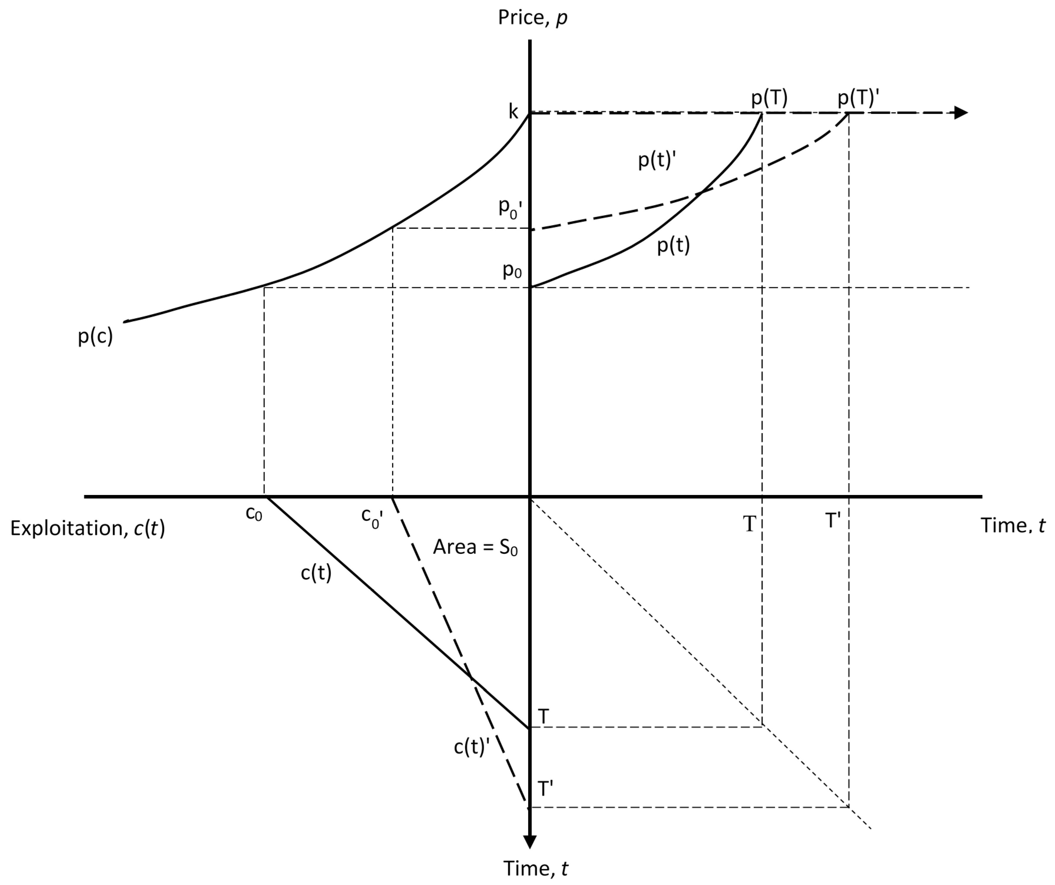
3.2. Technological Innovation

Both exploitation and the life of the safe operating space can be affected by technological innovation that reduce the economy’s dependence on and demand for using the various natural resources and pollution sinks that may comprise a safe operating space. For example, the safe operating space for climate change might be the global carbon budget, which is the cumulative amount of anthropogenic CO₂ emissions that would limit global warming to less than 2 °C [7,14,15]. Innovations that reduce greenhouse gas (GHG) emissions, such as carbon capture and sequestration, hybrid vehicles, GHG abatement technologies, and switching to renewables, would lessen depletion of the remaining 2 °C global carbon budget. Similarly, a safe operating space for land-system change could be set in terms of forested land as a percentage of original forest cover or potential forest [4]. Feeding a growing world population is expected to require an addition 3 to 5 million hectares (ha) of new cropland each year from now until 2030, which could contribute to additional clearing of 150 to 300 million ha in total area of natural forests [16]. Consequently, technologies that improve agricultural yields, foster sustainable management and generate zero net land degradation might reduce the pressure for cropland expansion and thus the demand for converting more natural forests [17].

Using diagrams to represent the modeling relationships developed previously, Figure 2 indicates the likely effects of a technological innovation that reduces the demand for exploiting a given safe operating space $S_0$. The diagram assumes a positive net rate of return $\mathsf{\rho }>0$, and consequently, $S_0$ is completely depleted in finite time T. The solid lines show the optimal exploitation and price paths before any innovation takes place. The upper right quadrant shows that the price path corresponding to (4), which rises exponentially at the rate ρ to end at the choke price k at time T. The upper left quadrant indicates the inverse demand curve for exploitation $p\left(c\right)$, which indicates that exploitation ceases at the choke price. As shown in the bottom left quadrant, given the demand curve and the price path, optimal exploitation $c\left(t\right)$ must begin at an initial level $c_0$ corresponding to $p_0$, decline over time, and eventually equal zero at time T when the choke price k is reached.

However, innovation can reduce the economy’s dependence on and demand for exploiting the given safe operating space $S_0$. In Figure 2, this is represented in the upper left quadrant by a shifting inward of the demand curve to ${p\left(c\right)}^{\prime }$, although the choke price remains at k. Given this change, the price path must move outward so that initial price ${p_0}^{\prime }$ and exploitation ${c_0}^{\prime }$ are lower, and thus the price must take longer to reach k. It follows that the lifetime of the safe operating space is extended, from T to T’. The new exploitation path ${c\left(t\right)}^{\prime }$ still depletes $S_0$ eventually, but it takes more time for this to occur. For example, in the case of an iso-elastic inverse demand function $p\left(c\right)=k{e}^{-\mathsf{\alpha }c}$, changes in the parameter α reflect the impact of innovation. As shown previously, for this demand curve that the optimal time for exploiting the safe operating space is $T={\left(\frac{2\mathsf{\alpha }{S}_0}{\mathsf{\rho }}\right)}^{\frac{1}{2}}$. It follows that $\frac{\partial p}{\partial \mathsf{\alpha }}<0$ and $\frac{\partial T}{\partial \mathsf{\alpha }}>0$, which are the effects depicted in Figure 2.

3.3. Stock Externalities

As noted previously, if the remaining safe operating space $S\left(t\right)$ includes maintenance of important habitats, ecosystems or biological species, it may generate wider social benefits, or “stock externalities”, such as biodiversity values, watershed protection, carbon sequestration and ecotourism. From condition (4), if these values are extremely large, then the markup v will be high, the net rate of return ρ earned from investing the proceeds from exploiting the safe operating space will be lower, and the price path $p\left(t\right)$ will evolve more slowly. It will take longer to exploit fully the remaining safe operating space. If stock externalities are extremely high, then the net rate of return ρ will approach zero, and $S\left(t\right)$ will be conserved indefinitely.

Figure 3 illustrates these effects. The solid lines show the optimal exploitation and price paths before any increase in values. More valuable stock externalities mean that v rises and ρ falls. The price path shifts so that initial price ${p_0}^{\prime }$ is higher, price rises much more slowly along the new price path ${p\left(t\right)}^{\prime }$, and the price takes longer to reach k. It follows that the lifetime of the safe operating space is extended, from T to T’. The new exploitation path ${c\left(t\right)}^{\prime }$ still depletes $S_0$ eventually, but it takes more time for this to occur. In the extreme case where stock externalities are so valuable, then the condition $\hspace{0.17em}\underset{\mathsf{\rho }\to 0}{Lim}T=\infty$ in (4) is reached, and the initial price immediately jumps to the choke price, i.e., $p_0=k$ and $c_0=0$. It is no longer optimal to exploit the safe operating space at all.

The outcome depicted in Figure 3 indicates why it is important to quantify and value any stock externality values associated with the remaining safe operating space available for human exploitation. If the safe operating space includes important habitats, ecosystems or biological species that generate wider social benefits, such as biodiversity values, watershed protection, carbon sequestration and ecotourism, then the inclusion of these values will delay full exploitation of the remaining $S\left(t\right)$, and perhaps extend its lifetime for significantly longer periods than if these additional stock externality values are ignored. Similar results are obtained by [18] through employing various competing land use models applied to ecosystems.

4. Discussion

A growing literature has focused on establishing a planetary boundary framework necessary to define a “safe operating space” for ensuring the sustainability of human economic activities and livelihoods [1,2,3,4,5,6]. Applying such a framework must take into account the uncertainty over thresholds, abrupt and irreversible change, and the magnitude of welfare impacts [4,8,13]. As we have emphasized in this paper, recognizing the need for planetary boundaries to limit human impacts on critical global sinks and resources is synonymous with the “strong sustainability” perspective in economics (Table 1). This view maintains that some forms of natural capital are essential, and thus cannot be substituted by reproducible and human capital; consequently, the sustainability goal of maintaining and enhancing the value of the aggregate capital stock requires preserving essential natural capital. By suggesting limits on nine damaging processes resulting from global human activity—climate change, loss of biosphere integrity, land-system change, freshwater use, biochemical flows, ocean acidification, atmospheric aerosol loading, stratospheric ozone depletion, and novel entities—the planetary boundary literature is arguing that key global sinks and resources are essential, may not be substituted, and thus are inviolate.

However, if planetary boundaries place limits on some uses of the global environment, this “safe operating space” must still be managed efficiently and sustainably [8]. Here, we have shown that, if the safe operating space defined by planetary boundaries is treated as a depletable stock, then the principles of weak sustainability should be applied (Table 1). That is, the safe operating space is a capital asset, and its sustainable management requires efficient use over time. Standard tools of natural resource management of an exhaustible resource economics can then be applied, and various conditions for optimal use, price paths, technological innovation and the presence of stock externalities can be explored.

Because our analysis treats any given safe operating space as an exhaustible resource exploited in finite time, optimal exploitation paths always end in eventual depletion of this asset. However, we also show that technological innovation and the presence of valuable stock externalities can extend the lifetime of the safe operating space—possibly even indefinitely. Innovations that reduce the economy’s dependence on and demand for using the various natural resources and pollution sinks that may comprise a safe operating space prolong its exploitation further into the future, and thus postpone eventual depletion. The remaining safe operating space may include habitats, ecosystems or biological species that generate wider social benefits, or “stock externalities”, such as biodiversity values, watershed protection, carbon sequestration and ecotourism. If the value of these additional social benefits rises, then the net rate of return earned from investing the proceeds from exploiting the safe operating space will be lower. Once again, less exploitation will occur, and depletion of the remaining safe operating space will be delayed.

These results suggest that policies associated with “greening” economic activity are likely to promote better stewardship of the safe operating space defined by planetary boundaries. For example, it has been argued that “making economies more sustainable requires urgent progress in three key policy areas: valuing the environment, accounting for the environment, and creating incentives for environmental improvement” [9] (p. 1).

The first two policy initiatives are essential to ensuring that the wider social benefits of stock externalities, especially those associated with valuable ecosystems, habitats and biodiversity, are properly valued and accounted for in environmental decision making. Valuing ecosystem goods and services has become a major focus for interdisciplinary collaboration between economists, ecologists and natural scientists, which offers hope for valuing many complex but environmental benefits, such as storm protection and flood mitigation by wetlands, soil and sedimentation control in watershed, fish diversity in coral reefs, and biodiversity of tropical forests [18]. These ecological values need also to be incorporated into our measures of economic wealth, so that we can more accurately account for the depreciation in valuable natural systems, resources and sinks that comprise our endowment of natural capital [9,10,11].

The third policy initiative is important for fostering innovations that reduce the economy’s dependence on and demand for using various natural resources and pollution sinks [9,10]. Today, the use of market-based instruments and other incentives to promote the “proper pricing” of pollution and natural resource use is gaining prevalence. Equally important is the removal of harmful subsidies that distort markets and foster excessive environmental degradation and resource use. Such price incentives are important to promoting innovations that reduce greenhouse gas (GHG) emissions, such as carbon capture and sequestration, hybrid vehicles, GHG abatement technologies, and switching to renewables [15]. Proper pricing could support the adoption of technologies that improve agricultural yields, foster sustainable management and generate zero net land degradation might reduce the pressure for cropland expansion and thus the demand for converting more natural forests [17].

However, price incentives may be necessary but not sufficient. Private investors tend to under-invest in the research and development (R&D) necessary to develop new “green” innovations, because they are unable to capture the full benefits of these advances as they rapidly spread throughout the economy and even to overseas competitors [10,19,20,21]. Overcoming this disincentive cannot be achieved solely through the use of price incentives but requires the simultaneous implementation of ‘‘technology-push policies”, such as R&D subsidies, public investments, protecting intellectual property, and other initiatives [10,19]. Such technology-push policies directly address the tendency of firms and industries to under-invest in green R&D, and thus are important complements to price incentives in reducing overall demand for resource use and pollution.

Finally, our analysis applies to the case where there is a well-defined safe operating space. As some proponents of the planetary boundaries framework have pointed out [2,4], the cumulative anthropogenic impacts on genetic diversity, nitrogen and phosphorous have led to such high risk of transgressing critical thresholds that no further human impacts should be tolerated. Although the individual planetary boundaries for genetic diversity, nitrogen and phosphorous may have been irrevocably breached, it may still be possible to define a safe operating space in other ways. For example, as the major threats to both the nitrogen and phosphorous cycles arises from fertilizer application in agriculture worldwide, it has been suggested that a biogeochemical planetary boundary can be set simultaneously for a combined nitrogen-phosphorous ratio, thus allowing a reasonable safe operating space to be delineated [4]. Similarly, Running [3] has proposed that several key planetary boundaries, including genetic diversity, can be captured in a single measurable global unit, which is net primary production. If scientists can determine reasonable planetary boundaries, our analysis shows that any resulting safe operating space should be treated as a capital asset, and consequently, it is relatively straightforward to develop the conditions for efficient and sustainable management of this depletable asset over time.

References

1. Lenton, T.M.; Held, H.; Kriegler, E.; Hall, J.W.; Lucht, W.; Rahmstorf, S.; Schellnhuber, H.J. Tipping elements in the Earth’s climate system. Proc. Natl. Acad. Sci. USA 2008, 105, 1786–1793. [Google Scholar] [CrossRef] [PubMed]
2. Rockström, J.; Steffen, W.; Noone, K.; Persson, A.; Chapin, A.S., III; Lambin, E.F.; Lenton, T.M.; Scheffer, M.; Foke, C.; Schellnhuber, H.J. A safe operating space for humanity. Nature 2009, 461, 472–475. [Google Scholar]
3. Running, S.W. A measurable planetary boundary for the biosphere. Science 2012, 337, 1458–1459. [Google Scholar] [CrossRef] [PubMed]
4. Steffen, W.; Richardson, K.; Rockström, J.; Cornell, S.E.; Fetzer, I.; Bennett, E.M.; Biggs, R.; Carpenter, S.R.; de Vries, W.; de Wit, E.A. Planetary Boundaries: Guiding Human Development on a Changing Planet. Available online: http://science.sciencemag.org/content/347/6223/1259855 (accessed on 16 October 2017).
5. Gerton, D.; Hoff, H.; Rockström, J.; Jägermeyr, J.; Kummu, M.; Pastor, A.V. Towards a revised planetary boundary for consumptive freshwater use: The role of environmental flow requirements. Curr. Opin. Sustain. 2013, 5, 551–558. [Google Scholar] [CrossRef]
6. Mace, G.M.; Reyers, B.; Alkemade, R.; Biggs, R.; Chapin, F.S., III; Cornell, S.E.; Díaz, S.; Jennings, S.; Leadley, P.; Mumby, P.J. Approaches to defining a planetary boundary for biodiversity. Glob. Environ. Chang. 2014, 28, 289–297. [Google Scholar] [CrossRef] [Green Version]
7. Intergovernmental Panel on Climate Change (IPCC). Climate Change 2014: Synthesis Report; Contribution of Working Groups I, II and III to the Fifth Assessment Report of the Intergovernmental Panel on Climate Change; Core Writing Team, Pachauri, R.K., Meyer, L.A., Eds.; IPCC: Geneva, Switzerland, 2014. [Google Scholar]
8. Smith, V.K. Environmental economics and the Anthropocene. Oxf. Res. Encycl. Environ. Sci. 2017. [Google Scholar] [CrossRef]
9. Barbier, E.B.; Markandya, A. A New Blueprint for a Green Economy; Routledge/Taylor & Francis: London, UK, 2013. [Google Scholar]
10. Barbier, E.B. Nature and Wealth: Overcoming Environmental Scarcity and Inequality; Palgrave MacMillan: London, UK, 2015. [Google Scholar]
11. Barbier, E.B. Sustainability and development. Annu. Rev. Resour. Econ. 2016, 8, 261–280. [Google Scholar] [CrossRef]
12. Daily, G.C.; Söderqvist, T.; Aniyar, S.; Arrow, K.; Dasgupta, P.; Ehrlich, P.R.; Folke, C.; Jansson, A.; Jansson, B.O.; Kautsky, N. The value of nature and the nature of value. Science 2000, 289, 395–396. [Google Scholar] [CrossRef] [PubMed]
13. Crépin, A.S.; Folke, C. The economy, the biosphere and planetary boundaries: Towards biosphere economics. Int. Rev. Environ. Econ. 2014, 8, 57–100. [Google Scholar] [CrossRef]
14. Barbier, E.B.; Burgess, J.C. Depletion of the global carbon budget: A user cost approach. Environ. Dev. Econ. 2017, 3, 1–16. [Google Scholar] [CrossRef]
15. Van der Ploeg, R. The Safe Carbon Budget; CESifo Working Paper No. 6620; Munich Society for the Promotion of Economic Research—CESifo: Munich, Germany, 2017. [Google Scholar]
16. Lambin, E.F.; Meyfroidt, P. Global land use change, economic globalization and the looming land scarcity. Proc. Natl. Acad. Sci. USA 2011, 108, 3465–3472. [Google Scholar] [CrossRef] [PubMed]
17. Grainger, A. Is land degradation neutrality feasible in dry areas? J. Arid Environ. 2015, 112, 14–24. [Google Scholar] [CrossRef]
18. Barbier, E.B. Capitalizing on Nature: Ecosystems as Natural Assets; Cambridge University Press: Cambridge, UK, 2011. [Google Scholar]
19. Goulder, L. Induced Technological Change and Climate Policy; Pew Center on Global Climate Change: Arlington, VA, USA, 2004. [Google Scholar]
20. Fankhauser, S.; Bowen, A.; Calel, R.; Dechezleprêtre, A.; Grover, D.; Rydge, J.; Sato, M. Who will win the green race? In search of environmental competitiveness and innovation. Glob. Environ. Chang. 2013, 23, 902–913. [Google Scholar] [CrossRef] [Green Version]
21. Clift, R.; Sim, S.; King, H.; Chenoweth, J.L.; Christie, I.; Clavreul, J.; Mueller, C.; Posthuma, L.; Boulay, A.M.; Chaplin-Kramer, R. The challenges of applying planetary boundaries as a basis for strategic decision-making in companies with global supply chains. Sustainability 2017, 9, 279. [Google Scholar] [CrossRef]
Figure 1. Setting the planetary boundary to define the safe operating space: (a) When past environmental responses (solid line curve) to human impacts are likely to provide a good indication of future responses (dotted line curve), the planetary boundary demarcating the safe operating space (vertical solid line) may be established relatively close to the predicted threshold (vertical dotted line); (b) When past environmental responses (solid line curve) are unlikely to provide a good indication of future responses (dotted line curves), and there is uncertainty over irreversible threshold effects, the desired planetary boundary (vertical solid line) may be set so that the safe operating space is relatively far from the predicted threshold (vertical dotted line).
Sustainability 09 01858 g001
Figure 2. The effect of innovations that reduce the demand for exploiting the safe operating space.
Sustainability 09 01858 g002
Figure 3. The effect of increases in the value of stock externalities associated with the safe operating space.
Sustainability 09 01858 g003