Strategy Analysis of Recycling and Remanufacturing by Remanufacturers in Closed-Loop Supply Chain

Abstract

The paper investigates interactions in a two-period closed-loop supply chain consisting of a single manufacturer and a single remanufacturer. In the context of recycling and remanufacturing by the remanufacturer, the manufacturer and remanufacturer choose different production strategies. By comparing the costs, profits and equilibrium quantity of supply chain members in decentralized and centralized models, we focus on the conditions under which the remanufacturer chooses to sell the remanufactured products and compete with the manufacturer. Different cooperative strategies can affect closed-loop supply chain decision-making. The article analyzes the impact of each cost and recycling rate on the productions and profits of the manufacturer and remanufacturer, and compares the total profits of members between two models. The sensitivity analysis of the models shows that the centralized model can be an effective way of achieving greater efficiency in terms of the overall supply chain. This study provides insights into the remanufacturing theory, which might guide remanufacturing operations and strategies.

1. Introduction

The concept of closed-loop supply chain (CLSC) was created as a result of the growing concerns about sustainable development in the world, which incorporates design, control, and operation of a system to maximize value creation over the entire lifecycle of a product with dynamic recovery of value from different types and volumes of returns over time [1]. Industry practices have been shown that remanufacturing in CLSC can help save costs, increase profits and boost competitive edge. Recycling and remanufacturing are conducive to developing good images for enterprises.

Remanufactured products can be produced by original equipment manufacturers (OEMs) as well as the independent operator (IO). In terms of the current purchasing modes of remanufactured products, manufacturers, retailers and remanufacturers can sell their products. With respect to OEM enterprises, markets of new and remanufactured products may have conflicts, and thus many OEMs are not active in producing remanufactured products. For example, Caterpillar Company separates the market of new products from that of the remanufactured products. The report of the Gartner Company shows that manufacturers are losing profits due to the competition from the low cost of remanufactured products. In 2010, they lost over USD 13 billion, and the potential threat forces manufacturers to reconsider whether they should also offer remanufactured products [2] to respond to the competition from the third party of remanufacturers. In practice, manufacturers have had themodes of selling remanufactured products [3,4]. The manufacturer and remanufacturer can cooperate and complement each other. It is worth noting that both the manufacturer and remanufacturer pursue cooperation because the manufacturer tends to boost their corporate image and expand their market share and the remanufacturer broadens the market; moreover, sales of remanufactured products by remanufacturer do not pose a great threat to the sales of new products by OEMs.

As we observe in practice, remanufactured automotive parts industry has a long-standing tradition of the third-party involvement. Although Ford and other major automotive manufacturers have endeavored to make inroads into reuse of parts, third-party players (e.g., Cardone Industries) have maintained a strong control on the automotive parts product acquisition market. Therefore, this article aims to model the interaction between the OEM and the remanufacturer, and analyzes the reasons for the competition and cooperation between them, thus providing some policy and management advice for businesses and governments.

This article adopts quantitative methodologies, and provides decentralized and centralized models on the condition of whether manufacturers and remanufacturers cooperate or not. Sensitivity analysis is deployed to show the reasons why supply chain members choose strategies when the cost parameters and recycling rate change. The remanufacturer recycling used products is the leader in the Stackelberg game (The Stackelberg game is a strategic game in economics in which the leader firm moves first and then the follower firms move sequentially. They compete on quantity. The Stackelberg game involves who determines the purchasing mode and improves the supply chain gaming theory in remanufacturing [3,5,6]. The problems can be solved by Lagrange function based on KKT (Karush–Kuhn–Tucker) conditions [7], which are necessary for a solution in nonlinear programming to be optimal, provided that some regularity conditions are satisfied).

This paper has three main objectives. Firstly, by applying the models of this paper, the CLSC members may acquire better management of products and coordination with new products, improving the CLSC efficiency (economically) and sustainability (environmentally). Secondly, our topic is related with environmental impact and waste recovery management, and hence our research highlights the importance of CLSC management. The results of this research support a decision maker during the selection of the proper strategies to put in place. The third objective is to provide a comprehensive and updated overview of CLSC strategies from the perspective of the remanufacturer.

The remainder of the paper is organized as follows. In Section 2, we present a review of literature. In Section 3, we provide the model description and build Model I of the centralized decisions. In Section 4, Model D of decentralized Strategies is constructed. In Section 6, we compare the centralized and decentralized models. In Section 7, conclusions are drawn and limitations are considered and the potential research orientations in the future are also taken into account.

2. Literature Review

CLSC has gained considerable attention during the recent years (Guide et al. [1]; Savaskan et al. [5]; Debo et al. [8]; Atasu et al. [9]; Wu [10]; Ma et al. [11]), the majority of research on the closed-loop supply chain focuses on the strategies of recycling and remanufacturing based on quantitative methodologies, and our research is no exception, concerning the operation of the CLSC from the remanufacturer’s view point.

Based on the research method of Cerchione et al. [12], Centobelli et al. [13], Centobelli et al. [14] and Rajeev et al. [15], the literature review consists of three major parts. The first part of the literature is concerned with the study of the feasibility of introducing remanufactured products into OEMs. In the second part, the competitive and collaborative strategies and diverse types of competition between OEMs and independent remanufacturers are considered. In the third part, compared with prior literature, the main contributions of this study are presented.

Souza et al. [16] and Govindan et al. [17] contribute to the study of CLSC. Battini et al. [18] show new research directions in the domain of CLSC management. These offer the opportunity to integrate their findings and draw a clear research framework in the area of CLSC.

The first mainstream research deals with the impact of external competition from independent remanufacturers on OEMs’ remanufacturing and competitive strategies. Ferrer et al. [19] and Ferrer et al. [20] analyze the critical conditions for OEMs to remanufacture to compete with manufacturers with double-oligarch monopolization. Ferguson et al. [21] develop the strategy for OEMs to compete with the independent remanufacturer when there is difference between new and remanufactured products. According to [22], it is very difficult for OEMs to enter the remanufacturing market after IOs’ monopoly. Giovanni et al. [23] consider a two-period CLSC game where a remanufacturer decides whether to exclusively manage the end-of-use product collection or to outsource it to either a retailer or a third party. Wu [24] develops a model of the closed-loop supply chain and considers OEMs’ and remanufacturer’s balanced prices and incentive measures. OEMs compete with remanufacturer intensively in recycling market and they compete on price in the market. Gan et al. [25] show that remanufacturing might not cannibalize the new product’s sales, if these two products are sold via different channels.

The topic of competitive and collaborative strategies between OEMs and independent remanufacturers has been gaining greater prominence in the literature. Karakayaliet al. [26] develop the decentralized and centralized models to determine the optimal recycling price, selling price of remanufactured products, and coordinate the decentralized supply chains. Jung et al. [27] compare and analyze the competition and cooperation between OEMs and the third-party remanufacturer. They reveal that competition among enterprises can accelerate the recycling rate and reduce pollution, whereas cooperation can increase enterprises’ profits. Chen et al. [28] study the competition and cooperation between OEMs and remanufacturers in stochastic demand. In the collaborative model, OEMs produce new and remanufactured products. In the competitive model, OEMs produce new products, while remanufacturers produce remanufactured products. According to [3], the profits in the cooperative model are higher than those in the competitive model. The collaborative model can be developed if remanufacturer’s profits are achieved. Wang and Xiong [4] reveal that the collaborative model benefits manufacturers, whereas the competitive model is conducive to remanufacturers and market expansion. However, from the perspective of revenues, the collaborative model is not necessarily superior to the competitive model. Scottish Government [29] allowed manufacturers to collaborate with remanufacturers to recycle used products. Wu [24] shows that it is common for the manufacturer and remanufacturer to cooperate in recycling used products. This has been rarely mentioned in previous studies, and hence it is likely to explore the competition and cooperation between the manufacturer and remanufacturer. In other words, the remanufacturer recycles used products and provides the recycled components for manufacturers and sell remanufactured products at the same time. They collaborate with the manufacturer in recycling market, whereas they compete in selling market. OEMs and remanufacturers can interact strategically and tactically through the strategies of price and quantity competition. Ma et al. [11] investigate interactions among different parties in a three-echelon closed-loop supply chain and focus on how cooperative strategies affect closed-loop supply chain decision-making. There are diverse types of competition between OEMs and remanufacturers, and product design strategy, recycle strategy and service strategy can handle remanufacturers’ competition very well [10,30,31]. Bulmus et al. [32] investigate the two-period model in which OEMs and independent remanufacturers compete in recycling and selling markets. OEMs’ recycling price depends on their own cost, which is different from the recycling price of the independent remanufacturer. Xiong et al. [33] analyze the performance of manufacturer-remanufacturing and supplier-remanufacturing in a decentralized closed-loop supply chain. Miao et al. [34] develop three kinds of decision models for closed-loop supply chain (CLSC), providing conditions under which one of these three collection strategies is optimal for different supply chain models.

Most previous studies investigate the strategies and operations of CLSC problems from the perspective of the OEMs. Compared with the previous studies, the main contributions of this paper are three-fold. Firstly, we consider the closed-loop supply chain in the mode of recycling and remanufacturing by the remanufacturer and investigate the impact of remanufacturing strategies on production and profits, which may reduce the operational cost of remanufacturing supply chains, thus boosting the collaboration efficiency of the remanufacturing supply chains. Secondly, few previous studies have discussed the strategies of purchasing competition and cooperation between the OEM and the remanufacturer from the perspective of the remanufacturer. Therefore, research on the feature of competition and cooperation in CLSC can shed light on the effective management of the remanufacturing industry. Finally, based on the recycling and remanufacturing mobile phones and automobiles, our research also provides insights to decision makers, and we show that consumer’s WTP and the cost for the remanufacturer’s product have an important effect on the strategies of CLSC members.

3. Model Description

This study considers a closed-loop supply chain in which the manufacturer competes and collaborates with the remanufacturer in two periods. In the first period, the manufacturer determines the output of new products, and there are no used products available for recycling. At the beginning of the second period, the remanufacturer recycles used products and produces remanufactured products and at the same time OEMs produce new products. A number of studies have claimed that consumers’ attitudes toward new and remanufactured products are identical (Savaskan et al. [5]; Bulmus et al. [6]; Atasu et al. [22]), in our study, there are some assumptions as follows:

Assumption 1: There are some differences between consumer attitude toward new and remanufactured products (Debo et al. [8]; Ferrer et al. [19]; Ferguson et al. [21]; Bulmus et al. [32]).

Assumption 2: There exists selling cost when the remanufacturer sells remanufactured products. Manufacturers own mature logistics network structure and thus they do not bear extra selling cost for selling remanufactured products. However, the remanufacturer mainly recycles and remanufactures the used products, and he does not have to sell remanufactured products. Therefore, it is assumed that the remanufacturer has to shoulder extra selling cost.

Assumption 3: The remanufacturer deploys recycling for used products in the first period to ensure the quantity and quality of recycling effectively.

Superscripts $i\in \left\{I,D\right\}$ represent the centralized and decentralized decisions by the manufacturer and remanufacturer, respectively. Superscripts $j\in \left\{a,b,c,d,e,f,g\right\}$ represent different Strategies, see

Table 1. Parameters setting.

Parameters	Meanings
$p_1$	The price of new products at which the manufacturer sells in the first period
$q_1$	The quantity of new products sold by the manufacturer in the first period
$p_{2n}$	The price of new products at which the manufacturer sells in the second period
$p_{2r}$	The price of remanufactured products at which the manufacturer sells in the second period
$p_{2i}$	The price of remanufactured products at which the remanufacturer sells in the second period
$q_{2n}$	The quantity of new products sold by the manufacturer in the second period
$q_{2r}$	The quantity of remanufactured products sold by the manufacturer in the second period
$q_{2i}$	The quantity of remanufactured products sold by the remanufacturer in the second period
$v$	The cost of recycling used products made in the first period and the production cost of remanufactured products in the second period
$c_n$	The production cost of new products
$c_r$	The cost of remanufactured products sold by the remanufacturer
$\delta$	Recyclable rate of used products
$\rho$	Consumers’ preference for remanufactured products in relation to new products
${\pi }_{ij}$	Participants’ profits in each period ( $i=1,2$；$j=M,R$), with $M$ as the manufacturer and $R$ as the remanufacturer

.

In the first period, the manufacturer produces only new products and there are no used products in the first period. In this study, the optimal strategy for the manufacturer to produce new products only can be achieved in the first period. Now, the relationship between demand quantity $q_1$ for new products and the sale price $p_1$ of new products is: $p_1=\left(1-q_1\right)$, and the demand function is the linear demand function mentioned by [8] and [21]. The manufacturer’s profit function is:

$$\underset{q_1}{\max }{\pi }_{1M}=\left(p_1-c_n\right)q_1$$

Substituting the sale price $p_1=\left(1-q_1\right)$ into the manufacturer’s profit function, the optimal production function of new products can be derived is $q_1=\frac{1-c_n}{2}$. The constraint is $q_1\ge 0$, and thus $c_n\le 1$ is required. At this moment, the sale price of new products is $p_1=\frac{1+c_n}{2}$, and the manufacturer’s optimal profit is ${\pi }_{1M}=\frac{{\left(1-c_n\right)}^2}{4}$. When the production of new and remanufactured products in the second period is analyzed, the default constraint here is $c_n\le 1$.

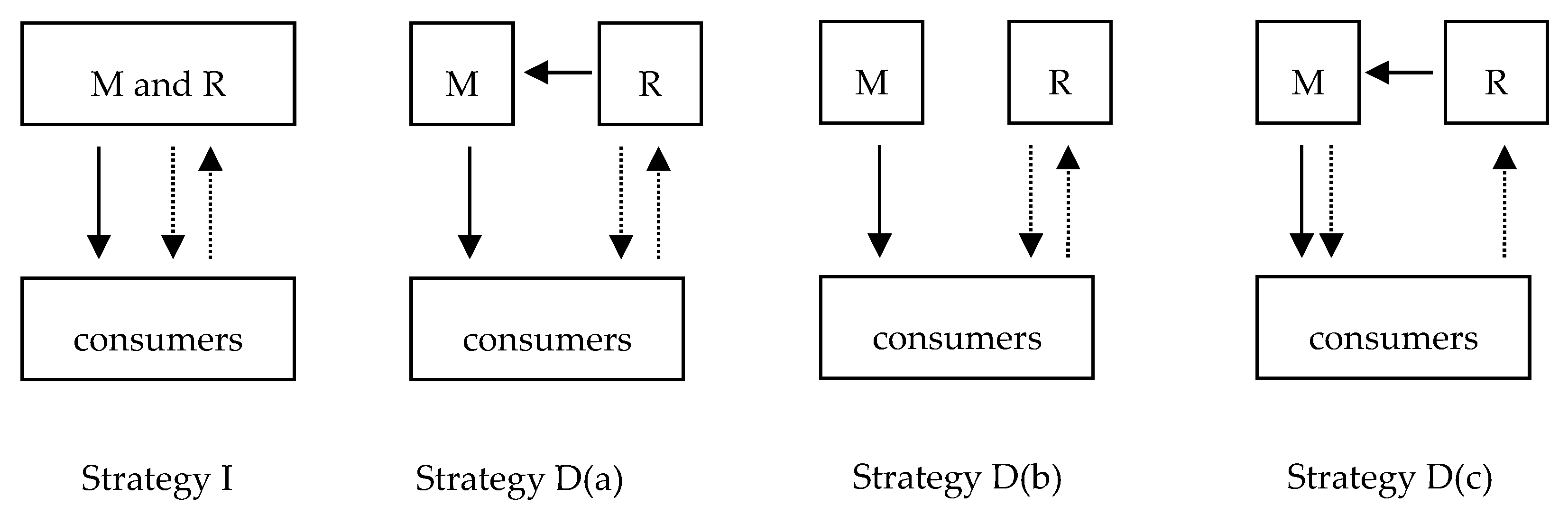
The second period involves recycling used products and producing remanufactured products. The remanufacturer serves as the main producer of remanufactured products with four strategies. Firstly, the remanufacturer collaborates with the manufacturer and makes joint decisions (Strategy I). Secondly, the remanufacturer sells part of remanufactured products and then resells part of remanufactured products to the manufacturer (Strategy D(a)). Thirdly, the remanufacturer sells all their remanufactured products, and competes with the manufacturer who produces new products (Strategy D(b)). Fourthly, the remanufacturer does not sell any remanufactured products (Strategy D(c)), and resells them to the manufacturer, taking advantage of manufacturer’s initial supply chain network to sell remanufactured products. Below involves the analyses of Model I in which the manufacturer and remanufacturer make joint decisions and Model D in which they make decentralized strategies.

In Figure 1, we list four strategies of the remanufacturer and manufacturer, with M as the manufacturer, with R as the remanufacturer, with the solid line as new products, with the dotted line downward as remanufactured products, with the dotted line upward as recycled products, and with the dotted line on the left as the wholesale remanufactured products.

3.1. Joint Strategies by Manufacturer and Remanufacturer—Model I

The manufacturer has mature networks and does not have to bear extra selling cost for remanufactured products. Hence, the profit function of the overall supply chains which consists of the manufacturer and remanufacturer is:

$${\pi }_{2M}=\left(p_{2n}-c_n\right)q_{2n}+\left(p_{2r}-v\right)q_{2r}$$

$$s.t.\{\begin{array}{c}\delta q_1\ge q_{2r}\\ q_{2n},q_{2r}\ge 0\end{array}$$

Based on KKT conditions, when the manufacturer and remanufacturer make jointly decisions, the optimal quantities and profits of new and remanufactured products is derived for the overall supply chain, see Appendix A (proof of Proposition 1).

Proposition 1. 

When the production cost of remanufactured products $v$ changes, the optimal quantities and profits of new and remanufactured products are derived for the overall supply chain. Additionally, below are three strategies achieved.

Strategy I-a: (i) When the production cost of remanufactured products $v$ satisfies $v<v_3^I$, the integrated manufacturers (the name is used when the manufacturer and remanufacturer jointly make decisions) determine the selling quantity of new products as $q_{2n}^{Ia}=\frac{\left(1-\delta \rho \right)\left(1-c_n\right)}{2}$; and they determine the selling quantity of remanufactured products as: $q_{2r}^{Ia}=\frac{\delta \left(1-c_n\right)}{2}$. Now, below are the profits of the overall supply chain: ${\pi }_{M2}^I=\frac{\left(1-\delta \rho \right){\left(1-c_n\right)}^2+\delta \left(1-c_n\right)\left[2c_n\rho -2v+\rho \left(1-c_n\right)\left(1-\delta +\delta \rho \right)\right]}{4}$.

Strategy I-b: (ii) When the production cost of remanufactured products $v$ satisfies $v_3^I\le v\le v_1^I$, the integrated manufacturers determine the selling quantity of new products as: $q_{2n}^{Ib}=\frac{1+v-\rho -c_n}{2\left(1-\rho \right)}$; and they determine the selling quantity of remanufactured products as: $q_{2r}^{Ib}=\frac{\rho c_n-v}{2\rho \left(1-\rho \right)}$. Now, below are the profits of the overall supply chain: ${\pi }_{M2}^I=\frac{\rho \left(1-c_n\right)\left(1+v-\rho -c_n\right)+\left(\rho c_n-v\right)\left(\rho -v\right)}{4\rho \left(1-\rho \right)}$.

Strategy I-c: (iii) When the production cost of remanufactured products $v$ satisfies $v_1^I<v$, the integrated manufacturers determine the selling quantity of new products as: $q_{2n}^{Ib}=\frac{1+v-\rho -c_n}{2\left(1-\rho \right)}$; the integrated manufacturers determine the selling quantity of new products as: $q_{2n}^{Ic}=\frac{\left(1-c_n\right)}{2}$; and they determine the selling quantity of remanufactured products as: $q_{2r}^{Ic}=0$. Now, below are the profits of the overall supply chain: ${\pi }_{M2}^I=\frac{{\left(1-c_n\right)}^2}{4}$.

In the above, $v_1^I=\rho c_n$, and $v_3^I=\rho c_n-\delta \rho \left(1-\rho \right)\left(1-c_n\right)$.

It can be seen from Proposition 1 that, no matter how low the production cost of remanufactured products is, new products will be manufactured in the overall supply chain. When $v_1^I<v$, the marginal profit of producing remanufactured products is too low and thus remanufactured products are not produced in the overall supply chain. When $v_3^I\le v\le v_1^I$, new and remanufactured products are produced in the overall supply chain. The production of remanufactured products will increase with the decrease of $v$, and the production of remanufactured products is maximal at $v_3^I$.

3.2. Sensitivity Analysis

Based on Proposition 1, the impact of cost parameters $c_n$, $v$, $c_r$ and $\delta$ on the pricing strategies of the remanufacturer in the overall supply chain is analyzed. Now, the impact of parameters on strategies can be shown in tables and figures. According to the rules of parameters set by [35] , to show the impact of each parameters variation on optimal strategies, the specific parameters setting is: $\rho =0.7$, $\delta =0.7$; when the impact of $c_n$ on the pricing strategy of remanufacturing among supply chain members is considered, assuming $v=0.2$; when the impact of $v$ on strategies is analyzed, assuming $c_n=0.5$.

In

Table 2. The impact of parameters variation on the optimal production in Model-I.

	${\mathit{q}}_{2\mathit{n}}^{\mathit{I}\mathit{a}}$	${\mathit{q}}_{2\mathit{n}}^{\mathit{I}\mathit{b}}$	${\mathit{q}}_{2\mathit{n}}^{\mathit{I}\mathit{c}}$	${\mathit{q}}_{2\mathit{r}}^{\mathit{I}\mathit{a}}$	${\mathit{q}}_{2\mathit{r}}^{\mathit{I}\mathit{b}}$	${\mathit{q}}_{2\mathit{r}}^{\mathit{I}\mathit{c}}$
$c_n$	$-$	$-$	$-$	$-$	$+$	$0$
$v$	$0$	$+$	$0$	$0$	$-$	$0$
$\delta$	$-$	$0$	$0$	$+$	$0$	$0$

, we list the impact of parameter variation on the optimal production in Model-I. ‘$+$’ represents that the optimal strategy grows when parameters increase; ‘$-$’ represents that the optimal strategy declines when parameters increase; and $0$ represents that the optimal strategy is not affected by parameters.

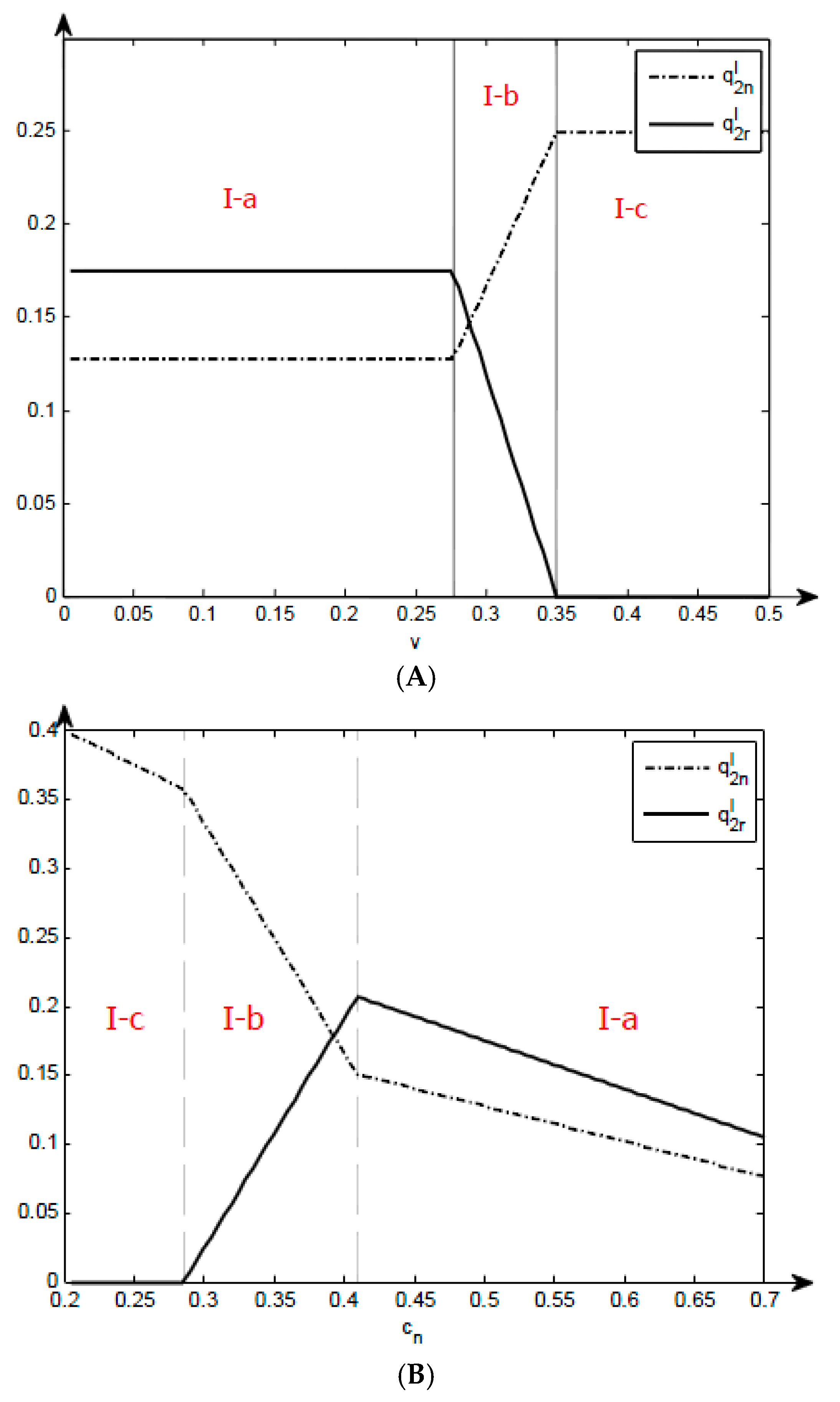
Figure 2A illustrates the impact of parameter $v$ variations on the optimal production in Model-I. Figure 2B illustrates the impact of parameter $c_n$ variations on the optimal production in Model-I. The regions bear tags with the format I-a, I-b, I-c, referring to three different strategies in different regions. The critical value of divisions is considered as the vertical axis, and the figure is divided into three ranges, in which Figure 2A from left to right correspond to Strategies I-a, I-b and I-c; Figure 2B from left to right correspond to Strategies I-c, I-b and I-a.

Table 2 and Figure 2B show that, as the cost of new products rises, output always declines. However, the output of remanufactured products declines with the rising cost of new products within the range of Strategy I-a, but it grows with the rising cost of new products within the range of Strategy I-b. There is no production of remanufactured products within the range of Strategy I-c, and the output of new products is not influenced by $c_n$. In the first period, the output of new products depends on $c_n$. In the second period, remanufactured products are made by recycling the products sold in the first period. As a result, the maximal quantity of used products available for remanufacturing declines, leading to the falling output of remanufactured products. The maximal output of remanufactured products is not maximal within the range of Strategy I-b, and new products can replace remanufactured products. The output of remanufactured products increases with the rise in cost of new products.

Figure 2A shows that the cost variations of remanufactured products affect production within the range of Strategy I-b. There is no production of remanufactured products within the range of Strategy I-c, and the output of new products is influenced by the cost of new products. The output of remanufactured products is maximal within the range of Strategy I-a, and the slight variation of $v$ does not break the equilibrium. There is no replacement effect, and the output of new products remains stable. The output of remanufactured products is not steady and is influenced by the cost of remanufactured products, and thus with the rising remanufacturing cost, the output of remanufactured products declines and that of new products increases.

When the output of remanufactured products is maximal, the variation of recycling rate has an impact on production. When the output of remanufactured products is not maximal, the variation of recycling rate does not influence the output of remanufactured or new products. The output of remanufactured products remains steady due to the limits of recycling rate of $\delta$ within the range of Strategy I-a. As a result, with the rising recycling rate, the overall supply chain is bound to choose to produce more remanufactured products and decrease the output of new products.

Figure 3A illustrates the impact of parameter $v$ variations on the optimal profits of the overall supply chains in Model I. Figure 3B illustrates the impact of parameter $c_n$ variations on the optimal profits of the overall supply chains in Model I. The regions bear tags with the format I-a, I-b, I-c, referring to three different strategies in different regions.

In

Table 3. The impact of parameter variation on the optimal profits of the overall supply chains in Model I.

	${\mathit{\pi }}_{2\mathit{M}}^{\mathit{I}\mathit{a}}$	${\mathit{\pi }}_{2\mathit{M}}^{\mathit{I}\mathit{b}}$	${\mathit{\pi }}_{2\mathit{M}}^{\mathit{I}\mathit{c}}$
$c_n$	$-$	$-$	$-$
$v$	$-$	$-$	$0$
$\delta$	$+$	$0$	$0$

and Figure 3A,B, it is clear that the profits of the overall supply chain always decline with $c_n$ increases. It can be seen in Table 3 that the output of remanufactured products increases within the scope of Strategy I-b, whereas revenues from the newly increased remanufactured products cannot compensate for the loss from the decreasing marginal cost of new products.

When the cost of remanufactured products increases, profits of the overall supply chain tend to decrease, if the output of remanufactured products is not 0. Within the scope of Strategy I-a, the output of new and remanufactured products is fixed, while the marginal profit of remanufactured products declines, and hence the total profits reduce.

In Strategy I-a, with the growing recycling rate, part of the resources for making new products get transferred to remanufactured products in the overall supply chain and the total profits of the overall supply chain increase with the high marginal profits of remanufactured products. The recycling rate does not affect the production in other scopes and it does not influence the profits naturally.

4. Strategies Analysis of the Decentralized Model D

In this section, it is assumed that remanufacturer is a leader in the Stackelberg game. The remanufacturer makes different strategies based on their production and selling cost, and provides the manufacturer with remanufactured products only. The remanufacturers provide the manufacturers with part of remanufactured products and sell part of remanufactured products, or sell all remanufactured products by themselves. In this section, the remanufacturer first determines the wholesale price of remanufactured products and the output and price of remanufactured products. Then, the manufacturer determines the output of new and remanufactured products. In this study, the reversal induction is deployed for solution.

In the second period, the manufacturer makes decisions on the sales of new and remanufactured products.

$$\underset{q_{2n},q_{2r}}{\max }{\pi }_{2M}=\left(p_{2n}-c_n\right)q_{2n}+\left(p_{2r}-w_{2r}\right)q_{2r}$$

Based on KKT conditions, the optimal quantities and profits of new and remanufactured products sold by manufacturer are derived, see Appendix B (proof of Proposition 2).

Proposition 2. 

When the wholesale price $w_{2r}$ of remanufactured products varies, the manufacturer determines the selling quantity of new products as $q_{2n}^D$ . Additionally, below are the three strategies adopted by the manufacturer.

In

Table 4. Manufacturer’s optimal sales of new and remanufactured products in Model D.

	${\mathit{q}}_{2\mathit{n}}^{\mathit{D}}$	${\mathit{q}}_{2\mathit{r}}^{\mathit{D}}$
$w_1^D<w_{2r}$	$\frac{1-c_n-\rho q_{2i}}{2}$	$0$
$w_3^D\le w_{2r}\le w_1^D$	$\frac{1+w_{2r}-c_n-\rho }{2\left(1-\rho \right)}$	$-\frac{\rho q_{2i}\left(1-\rho \right)+w_{2r}-c_n\rho }{2\rho \left(1-\rho \right)}$
$w_{2r}<w_3^D$	$\frac{\left(1-\delta \rho \right)\left(1-c_n\right)}{2}+\frac{\rho q_{2i}}{2}$	$\frac{\delta \left(1-c_n\right)}{2}-q_{2i}$

, it is clear that the quantity of remanufactured products sold by the remanufacturer does not affect the manufacturer’s choice of selling strategies, whereas the wholesale prices of remanufactured products determined by remanufacturers can exert an impact on manufacturer’s strategies. However, the quantity of remanufactured products sold by the remanufacturer can influence the product output under specific strategies. With the decrease of $w_{2r}$, the manufacturer takes three strategies: $q_{2r}^D=0$, $0<q_{2r}^D<\delta q_1-q_{2i}$ and $q_{2r}^D=\delta q_1-q_{2i}$, and the output of new products is constantly not 0.

In Table 4, $w_1^D=c_n\rho -\rho q_{2i}\left(1-\rho \right)$, and $w_3^D=\rho \left[c_n\left(1+\delta -\delta \rho \right)+\left(1-\rho \right)\left(q_{2i}-\delta \right)\right]$.

In the first stage, the remanufacturer determines the quantity of remanufactured products they will sell and the wholesale price of remanufactured products they resell to the manufacturer.

$$\underset{q_{2i},w_{2r}}{\max }{\pi }_{2R}=\left(w_{2r}-v\right)q_{2r}+\left(p_{2i}-c_r-v\right)q_{2i}$$

Based on KKT conditions, the optimal quantities of remanufactured product sold by remanufacturer are derived, see Appendix C (proof of Proposition 3).

Proposition 3. 

When the production cost $v$ of remanufactured products and the selling cost $c_r$ of the remanufacturer vary, the remanufacturer determines the selling quantity of remanufactured products as $q_{2i}^D$ . In addition, below are the strategies adopted by the remanufacturer.

• In Case I, with $0\le v<v_1^D$,

  $$c_3^D-c_1^D=v-c_n\rho +\delta \rho \left(1-\rho \right)\left(1-c_n\right)<-\delta \rho \left(1-\rho \right)\left(1-c_n\right)\le 0$$

  $$c_3^D-c_2^D=v-c_n\rho -\frac{\delta {\rho }^2\left(1-c_n\right)}{2}\le 0$$

  when $c_r<c_3^D$, the remanufacturer opts for the strategy of $q_{2i}^D=\frac{\delta \left(1-c_n\right)}{2}$.
• In Case II, with $v_1^D\le v\le v_2^D$,

  $$c_3^D-c_1^D=v-c_n\rho +\delta \rho \left(1-\rho \right)\left(1-c_n\right)\le 0$$

  when $c_r<c_3^D$, the remanufacturer opts for the strategy of $q_{2i}^D=\frac{\delta \left(1-c_n\right)}{2}$.
• In Case III, with $v_2^D<v\le v_3^D$,

  $$c_8^D-c_1^D=\frac{\delta \rho \left(1-c_n\right)\left(2-\rho \right)}{2}-\frac{\left(2-\rho \right)\left(c_n\rho -v\right)}{2\left(1-\rho \right)}>0$$

  $$c_8^D-c_2^D=-\frac{\left(2-\rho \right)\left(c_n\rho -v\right)}{2\left(1-\rho \right)}\le 0$$

  when $c_r<c_1^D$, the remanufacturer opts for the strategy of $q_{2i}^D=\frac{\delta \left(1-c_n\right)}{2}$; with $c_1^D\le c_r\le c_8^D$, the remanufacturer choose the strategy of $q_{2i}^D=\frac{\rho \left(1+c_n\right)-2\left(c_r+v\right)}{2\rho \left(2-\rho \right)}$.
• In Case IV, with $v_3^D<v$,
  when $c_r<c_1^D$, the remanufacturer opts for the strategy of $q_{2i}^D=\frac{\delta \left(1-c_n\right)}{2}$, whereas, when $c_1^D\le c_r\le c_2^D$, the remanufacturer opts for the strategy of $q_{2i}^D=\frac{\rho \left(1+c_n\right)-2\left(c_r+v\right)}{2\rho \left(2-\rho \right)}$. When $c_2^D<c_r$, the remanufacturer opts for the strategy of $q_{2i}^I=0$.

Based on the conclusions in Appendix C (

Table A2. The remanufacturer’s optimal sales and wholesale prices of remanufactured products in Model D.

	${\mathit{q}}_{2\mathit{i}}^{\mathit{D}}$	${\mathit{w}}_{2\mathit{r}}^{\mathit{D}}$
$v_3^D<v$ and $c_2^D<c_r$	$0$	none
$v_3^D<v$ and $c_1^D\le c_r\le c_2^D$ or $v_2^D<v\le v_3^D$ and $c_1^D\le c_r\le c_8^D$	$\frac{\rho \left(1+c_n\right)-2\left(c_r+v\right)}{2\rho \left(2-\rho \right)}$	none
$0\le \mathrm{v}<v_2^D$ and $c_r<c_3^D$ or $v_2^D<v$ and $c_r<c_1^D$	$\frac{\delta \left(1-c_n\right)}{2}$	none
$v_2^D<v\le v_3^D$ and $c_8^D\le c_r\le c_7^D$ or $v_1^D\le \mathrm{v}\le v_2^D$ and $c_5^D\le c_r\le c_7^D$	$\frac{\rho -2c_r-v}{2\rho }$	$\frac{\rho c_n+v}{2}$
$0\le \mathrm{v}\le v_1^D$ and $c_3^D\le c_r\le c_4^D$ or $v_1^D\le \mathrm{v}\le v_2^D$ and $c_3^D\le c_r\le c_5^D$	$-\frac{c_r}{\rho \left(2-\rho \right)}+\frac{\left(1-c_n\right)\left(1+2\delta -2\delta \rho \right)}{2\left(2-\rho \right)}$	$c_n\rho -\frac{c_r\left(1-\rho \right)}{\left(2-\rho \right)}+\frac{\rho \left(1-\rho \right)\left(1-2\delta \right)\left(1-c_n\right)}{2\left(2-\rho \right)}$
$v_1^D\le \mathrm{v}\le v_3^D$ and $c_r>c_7^D$	$0$	$\frac{v+c_n\rho }{2}$
$0\le \mathrm{v}<v_1^D$ and $c_4^D<c_r$	$0$	$c_n\rho -\delta \rho \left(1-\rho \right)\left(1-c_n\right)$

and

Table A3. The remanufacturer’s optimal sales of new and remanufactured products in Model D.

	${\mathit{q}}_{2\mathit{n}}^{\mathit{D}}$	${\mathit{q}}_{2\mathit{r}}^{\mathit{D}}$
$v_3^D<v$ and $c_2^D<c_r$	$\frac{\left(1-c_n\right)}{2}$	$0$
$v_3^D<v$ and $c_1^D\le c_r\le c_2^D$ or $v_2^D<v\le v_3^D$ and $c_1^D\le c_r\le c_8^D$	$\frac{2\left(c_r+v\right)+4\left(1-c_n\right)+\rho \left(c_n-3\right)}{4\left(2-\rho \right)}$	$0$
$0\le \mathrm{v}<v_2^D$ and $c_r<c_3^D$ or $v_2^D<v$ and $c_r<c_1^D$	$\frac{\left(2-\rho \delta \right)\left(1-c_n\right)}{4}$	$0$
$v_2^D<v\le v_3^D$ and $c_8^D\le c_r\le c_7^D$ or $v_1^D\le \mathrm{v}\le v_2^D$ and $c_5^D\le c_r\le c_7^D$	$\frac{1}{2}+\frac{v}{4\left(1-\rho \right)}-\frac{c_n\left(2-\rho \right)}{4\left(1-\rho \right)}$	$\frac{c_r}{2\rho }-\frac{1}{4}+\frac{c_n-v}{4\left(1-\rho \right)}$
$0\le \mathrm{v}<v_1^D$ and $c_3^D\le c_r\le c_4^D$ or $v_1^D\le \mathrm{v}\le v_2^D$ and $c_3^D\le c_r\le c_5^D$	$-\frac{c_r}{2\left(2-\rho \right)}+\frac{\left(1-c_n\right)\left(4-\rho -2\delta \rho \right)}{4\left(2-\rho \right)}$	$\frac{c_r}{\rho \left(2-\rho \right)}-\frac{\left(1-\rho \delta \right)\left(1-c_n\right)}{2\left(2-\rho \right)}$
$v_1^D\le \mathrm{v}\le v_3^D$ and $c_r>c_7^D$	$\frac{1}{2}+\frac{v}{4\left(1-\rho \right)}-\frac{c_n\left(2-\rho \right)}{4\left(1-\rho \right)}$	$\frac{c_n\rho -v}{4\rho \left(1-\rho \right)}$
$0\le \mathrm{v}<v_1^D$ and $c_4^D<c_r$	$\frac{\left(1-\rho \delta \right)\left(1-c_n\right)}{2}$	$\frac{\delta \left(1-c_n\right)}{2}$

), Proposition 4 is as follows.

Proposition 4. 

When the production cost $v$ of remanufactured products and the selling cost $c_r$ of remanufactured products vary, the manufacturer determines the selling quantity of new products as $q_{2n}^D$ and the quantity of remanufactured products as $q_{2r}^D$. The remanufacturer determines the selling quantity of remanufactured products as $q_{2i}^D$. In addition, below are the strategies adopted by the manufacturer and remanufacturer.

Strategy D-a

  When $v_3^D<v$ and $c_2^D<c_r$,

  $q_{2n}^{Da}=\frac{\left(1-c_n\right)}{2}$, $q_{2r}^{Da}=0$, and $q_{2i}^{Da}=0$, while $w_{2r}^{Da}$ does not exist.

Strategy D-b

  When $v_3^D<v$ and $c_1^D\le c_r\le c_2^D$ or $v_2^D<v\le v_3^D$ and $c_1^D\le c_r\le c_8^D$,

  $q_{2n}^{Db}=\frac{2\left(c_r+v\right)+4\left(1-c_n\right)+\rho \left(c_n-3\right)}{4\left(2-\rho \right)}$, $q_{2r}^{Db}=0$, and $q_{2i}^{Db}=\frac{\rho \left(1+c_n\right)-2\left(c_r+v\right)}{2\rho \left(2-\rho \right)}$, while $w_{2r}^{Db}$ does not exist.

Strategy D-c

  When $0\le v<v_2^D$ and $c_r<c_3^D$ or $v_2^D<v$ and $c_r<c_1^D$,

  $q_{2n}^{Dc}=\frac{\left(2-\rho \delta \right)\left(1-c_n\right)}{4}$, $q_{2r}^{Dc}=0$, and $q_{2i}^{Dc}=\frac{\delta \left(1-c_n\right)}{2}$, while $w_{2r}^{Dc}$ does not exist.

Strategy D-d

  When $v_2^D<v\le v_3^D$ and $c_8^D\le c_r\le c_7^D$ or $v_1^D\le v\le v_2^D$ and $c_5^D\le c_r\le c_7^D$,

  $q_{2n}^{Dd}=\frac{1}{2}+\frac{v}{4\left(1-\rho \right)}-\frac{c_n\left(2-\rho \right)}{4\left(1-\rho \right)}$, $q_{2r}^{Dd}=\frac{c_r}{2\rho }-\frac{1}{4}+\frac{c_n-v}{4\left(1-\rho \right)}$, $q_{2i}^{Dd}=\frac{\rho -2c_r-v}{2\rho }$, and $w_{2r}^{Dd}=\frac{\rho c_n+v}{2}$ are derived.

Strategy D-e

  When $0\le v\le v_1^D$ and $c_3^D\le c_r\le c_4^D$ or $v_1^D\le v\le v_2^D$ and $c_3^D\le c_r\le c_5^D$,

  $q_{2n}^{De}=-\frac{c_r}{2\left(2-\rho \right)}+\frac{\left(1-c_n\right)\left(4-\rho -2\delta \rho \right)}{4\left(2-\rho \right)}$, $q_{2r}^{De}=\frac{c_r}{\rho \left(2-\rho \right)}-\frac{\left(1-\rho \delta \right)\left(1-c_n\right)}{2\left(2-\rho \right)}$, $q_{2i}^{De}=-\frac{c_r}{\rho \left(2-\rho \right)}+\frac{\left(1-c_n\right)\left(1+2\delta -2\delta \rho \right)}{2\left(2-\rho \right)}$, and $w_{2r}^{De}=c_n\rho -\frac{c_r\left(1-\rho \right)}{\left(2-\rho \right)}+\frac{\rho \left(1-\rho \right)\left(1-2\delta \right)\left(1-c_n\right)}{2\left(2-\rho \right)}$ are derived.

Strategy D-f

  When $v_1^D\le v\le v_3^D$ and $c_r>c_7^D$,

  $q_{2n}^{Df}=\frac{1}{2}+\frac{v}{4\left(1-\rho \right)}-\frac{c_n\left(2-\rho \right)}{4\left(1-\rho \right)}$, $q_{2r}^{Df}=\frac{c_n\rho -v}{4\rho \left(1-\rho \right)}$, $q_{2i}^{Df}=0$, and $w_{2r}^{Df}=\frac{v+c_n\rho }{2}$ are derived.

Strategy D-g

  When $0\le v<v_1^D$ and $c_4^D<c_r$,

  $q_{2n}^{Dg}=\frac{\left(1-\delta \rho \right)\left(1-c_n\right)}{2}$, $q_{2r}^{Dg}=\frac{\delta \left(1-c_n\right)}{2}$, $q_{2i}^{Dg}=0$, and $w_{2r}^{Dg}=c_n\rho -\delta \rho \left(1-\rho \right)\left(1-c_n\right)$ are derived.

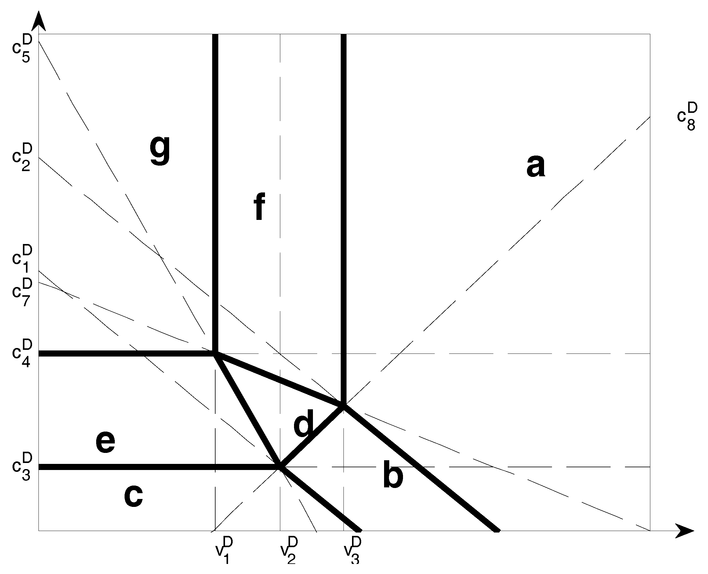
Figure 4 illustrates remanufacturer’s strategies in different remanufacturing costs $c_1^D$, $c_2^D$ … $c_7^D$ and selling costs $v_1^D$, $v_2^D$ , $v_3^D$ in Model D. The regions bear tags with the format a, b, c, d, e, f, g, referring to three different strategies in different regions.

The Strategies above are based on $c_n\ge \frac{2\delta \rho \left(1-\rho \right)}{\rho +2\delta \rho \left(1-\rho \right)}$ to ensure that $v_1^D$, $v_2^D$ and $v_3^D$ are greater than 0. When $\frac{\delta \rho \left(1-\rho \right)}{\rho +\delta \rho \left(1-\rho \right)}<c_n<\frac{2\delta \rho \left(1-\rho \right)}{\rho +2\delta \rho \left(1-\rho \right)}$, $v_1^D<0$ is derived; now, the condition of $0\le v<v_1^D$ in the strategy does not exist. In other words, Strategy D-g does not exist. When $0<c_n\le \frac{\delta \rho \left(1-\rho \right)}{\rho +\delta \rho \left(1-\rho \right)}$, $v_1^D,v_2^D<0$ is derived, the conditions of $0\le v<v_1^D$ and $v_1^D<v\le v_2^D$ in the strategy do not exist, i.e., Strategies of D-g and D-e do not exist.

Proposition 4 and Figure 4 show that the manufacturer’s and remanufacturer’s strategies depend on the remanufacturing and selling costs. The manufacturer and remanufacturer are interdependent. (1) When the remanufacturing cost is relatively lower, the output of remanufactured products is maximal. With different selling costs, there are differences in proportions between the products sold by the remanufacturer and those resold to the manufacturer. With the rising cost of selling, the remanufacturer tends to resell remanufactured products to the manufacturer. (2) When the remanufacturing cost is relatively higher and selling cost is relatively lower, the remanufacturer chooses to recycle used products, remanufacture and sell the products. Direct sales and reselling require that the remanufacturer recycles used products and remanufactures. If remanufacturing costs are too high, the profits of remanufactured products are too low or even zero. Hence, the remanufacturer certainly does not produce remanufactured products. (3) When selling cost is extremely low, the remanufacturer tends to sell remanufactured products directly. The reason is that the manufacturer takes part of the profits of remanufactured products if remanufactures resell their products and thus the remanufacturer’s profits decline. As a result, with extremely low selling costs, the remanufacturer sells all remanufactured products and competes with manufacturer completely. (4) When selling cost is moderate and remanufacturing costs are relatively low, the remanufacturer sells their products directly and resells part of products to the manufacturer. Now, the manufacturer competes and collaborates with the remanufacturer. (5) When selling cost is relatively high, the remanufacturers’ profits are too low from direct sales, and thus they resell their products to the manufacturer and focus on recycling. (6) The cost of new products also exerts an influence on remanufacturer’s strategies. The strategies above emerge if the costs of new products are extremely high. The reason is that the manufacturer who produces new products squeezes the market with relatively low cost of new products, and the consumer willingness to pay for the remanufactured product is lower than that of new products. If the manufacturer lowers the price of new products, the output of remanufactured products by the remanufacturer is bound to decline. At the same time, the decreasing cost of new products leads to the rising quantity of new products in the first period. The quantity of remanufactured products increases and thus it is difficult for the output of remanufactured products to grow.

According to the manufacturer’s profit function, ${\pi }_{2M}=\left(p_{2n}-c_n\right)q_{2n}+\left(p_{2r}-w_{2r}\right)q_{2r}$, and the remanufacturer’s profit function, ${\pi }_{2R}=\left(w_{2r}-v\right)q_{2r}+\left(p_{2i}-c_r-v\right)q_{2i}$, the optimal manufacturer’s and remanufacturer’s profits in different production and selling costs of remanufactured products are derived, as shown in Appendix C (

Table A4. The manufacturer’s and remanufacturer’s optimal profits in Model D.

	${\mathit{\pi }}_{2\mathit{M}}^{\mathit{D}}$	${\mathit{\pi }}_{2\mathit{R}}^{\mathit{D}}$
$v_3^D<v$ and $c_2^D<c_r$	$\frac{{\left(1-c_n\right)}^2}{4}$	$0$
$v_3^D<v$ and $c_1^D\le c_r\le c_2^D$ or $v_2^D<v\le v_3^D$ and $c_1^D\le c_r\le c_8^D$	$\frac{{\left(4-4c_n-3\rho +2v+2c_r+c_n\rho \right)}^2}{16{\left(2-\rho \right)}^2}$	$\frac{{\left(c_n\rho +\rho -2v-2c_r\right)}^2}{8\rho \left(2-\rho \right)}$
$0\le \mathrm{v}<v_2^D$ and $c_r<c_3^D$ or $v_2^D<v$ and $c_r<c_1^D$.	$\frac{{[\left(2-\rho \delta \right)\left(1-c_n\right)]}^2}{16}$	$\frac{\delta \rho \left(1-c_n^2\right)}{4}-\frac{\rho \left(2-\rho \right){\left[\delta \left(1-c_n\right)\right]}^2}{8}-\frac{\delta \left(1-c_n\right)\left(c_r+v\right)}{2}$
$v_2^D<v\le v_3^D$ and $c_8^D\le c_r\le c_7^D$ or $v_1^D\le \mathrm{v}\le v_2^D$ and $c_5^D\le c_r\le c_7^D$	$\begin{array}{l}\left[\frac{2c_r+\rho -\rho c_n}{4}\right]\left[\frac{c_r}{2\rho }-\frac{1}{4}+\frac{c_n-v}{4\left(1-\rho \right)}\right]\\ +\left[\frac{2+v+2c_r-2c_n-\rho }{4}\right][\frac{2+v+\rho c_n-2c_n-2\rho }{4\left(1-\rho \right)}]\end{array}$	$\begin{array}{l}\left[\frac{c_r}{2\rho }-\frac{1}{4}+\frac{c_n-v}{4\left(1-\rho \right)}\right]\left[\frac{\rho c_n-v}{2}\right]\\ +\left[\frac{\rho -2c_r-v}{2\rho }\right][\frac{c_n\rho +\rho -2v-2c_r}{4}]\end{array}$
$0\le \mathrm{v}<v_1^D$ and $c_3^D\le c_r\le c_4^D$ or $v_1^D\le \mathrm{v}\le v_2^D$ and $c_3^D\le c_r\le c_5^D$	$\begin{array}{l}\frac{\left[\left(1-c_n\right)\left(4-\rho -2\delta \rho \right)-2c_r\right]\left[2c_r+\left(1-c_n\right)\left(4+2\delta {\rho }^2-3\rho -2\delta \rho \right)\right]}{16{\left(2-\rho \right)}^2}\\ +\frac{\left[2c_r-\rho \left(1-\rho \delta \right)\left(1-c_n\right)\right]\left[\rho +2c_r-c_n\rho \right]}{8\rho \left(2-\rho \right)}\end{array}$	$\begin{array}{l}\frac{2c_r-\rho \left(1-\rho \delta \right)\left(1-c_n\right)}{2\rho \left(2-\rho \right)}[c_n\rho -\frac{c_r\left(1-\rho \right)}{\left(2-\rho \right)}\\ +\frac{\rho \left(1-\rho \right)\left(1-2\delta \right)\left(1-c_n\right)}{2\left(2-\rho \right)}-v]\\ +\frac{\rho \left(1-c_n\right)\left(1+2\delta -2\delta \rho \right)-2c_r}{2\rho \left(2-\rho \right)}[c_n\rho \\ +\frac{\rho \left(1-c_n\right)\left(4-4\delta -3\rho +4\delta \rho \right)}{4\left(2-\rho \right)}\\ -\frac{c_r\left(4-3\rho \right)}{2\left(2-\rho \right)}-v]\end{array}$
$v_1^D\le \mathrm{v}\le v_3^D$ and $c_r>c_7^D$	$\frac{\left(c_n\rho -v\right)\left(2\rho -v-c_n\rho \right)}{16\rho \left(1-\rho \right)}+\frac{\left(1-c_n\right)}{2}[\frac{1}{2}+\frac{v}{4\left(1-\rho \right)}-\frac{c_n\left(2-\rho \right)}{4\left(1-\rho \right)}]$	$\frac{{\left(c_n\rho -v\right)}^2}{8\rho \left(1-\rho \right)}$
$0\le \mathrm{v}<v_1^D$ and $c_4^D<c_r$	$\frac{\left(1+\rho {\delta }^2-{\rho }^2{\delta }^2\right){\left(1-c_n\right)}^2}{4}$	$[\frac{\delta \left(1-c_n\right)}{2}][c_n\rho -\delta \rho \left(1-\rho \right)\left(1-c_n\right)-v]$

).

5. Sensitivity Analysis

Based on Proposition 2, the impact of cost parameters of $c_n$, $v,c_r$ and $\delta$ on the remanufacturer’ sand manufacturer’s pricing strategies on remanufacturing is analyzed. Now, the impact of measuring parameters on strategies can be shown in tables and figures. According to the rules of parameters setting by Xiong et al. [35], to show the impact of each parameters variation on optimal Strategies, the specific parameters setting is: $\rho =0.7$, $\delta =0.7$, $c_n=0.5$, and $c_r$ and $v$ change within the range of 0 and 0.5.

Table 5. The impact of parameter variation on remanufacturer’s optimal strategies in Model D.

	${\mathit{w}}_{\mathbf{2}\mathit{r}}^{\mathit{D}\mathit{a}}$	${\mathit{w}}_{\mathbf{2}\mathit{r}}^{\mathit{D}\mathit{b}}$	${\mathit{w}}_{\mathbf{2}\mathit{r}}^{\mathit{D}\mathit{c}}$	${\mathit{w}}_{\mathbf{2}\mathit{r}}^{\mathit{D}\mathit{d}}$	${\mathit{w}}_{\mathbf{2}\mathit{r}}^{\mathit{D}\mathit{e}}$	${\mathit{w}}_{\mathbf{2}\mathit{r}}^{\mathit{D}\mathit{f}}$	${\mathit{w}}_{\mathbf{2}\mathit{r}}^{\mathit{D}\mathit{g}}$
$c_n$	$0$	$0$	$0$	$+$	$+$	$+$	$+$
$\mathrm{v}$	$0$	$0$	$0$	$+$	$0$	$+$	$0$
$c_r$	$0$	$0$	$0$	$0$	$-$	$0$	$0$
$\mathsf{\delta }$	$0$	$0$	$0$	$0$	$-$	$0$	$-$
	${\mathit{q}}_{\mathbf{2}\mathit{i}}^{\mathit{D}\mathit{a}}$	${\mathit{q}}_{\mathbf{2}\mathit{i}}^{\mathit{D}\mathit{b}}$	${\mathit{q}}_{\mathbf{2}\mathit{i}}^{\mathit{D}\mathit{c}}$	${\mathit{q}}_{\mathbf{2}\mathit{i}}^{\mathit{D}\mathit{d}}$	${\mathit{q}}_{\mathbf{2}\mathit{i}}^{\mathit{D}\mathit{e}}$	${\mathit{q}}_{\mathbf{2}\mathit{i}}^{\mathit{D}\mathit{f}}$	${\mathit{q}}_{\mathbf{2}\mathit{i}}^{\mathit{D}\mathit{g}}$
$c_n$	$0$	$+$	$-$	$0$	$-$	$0$	$0$
$\mathrm{v}$	$0$	$-$	$0$	$-$	$0$	$0$	$0$
$c_r$	$0$	$-$	$0$	$-$	$-$	$0$	$0$
$\mathsf{\delta }$	$0$	$0$	$+$	$0$	$+$	$0$	$0$

lists the impact of parameter ($c_n$, $c_r$, $v$ and $\delta$) variation on remanufacturer’s optimal strategies in Model D.

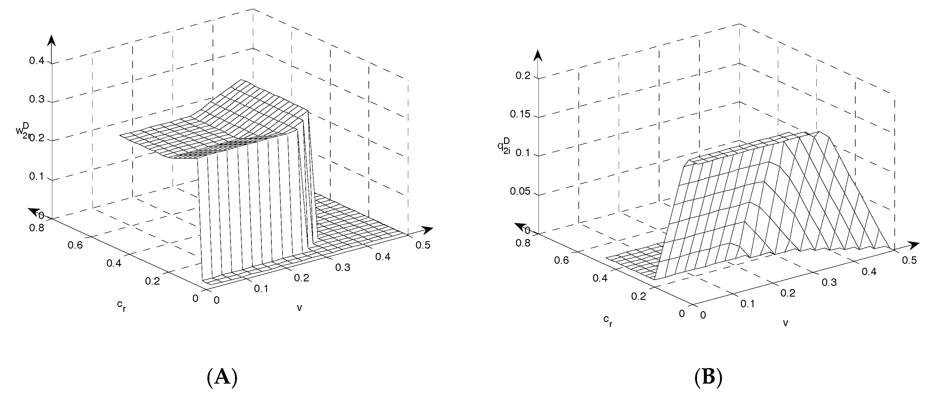
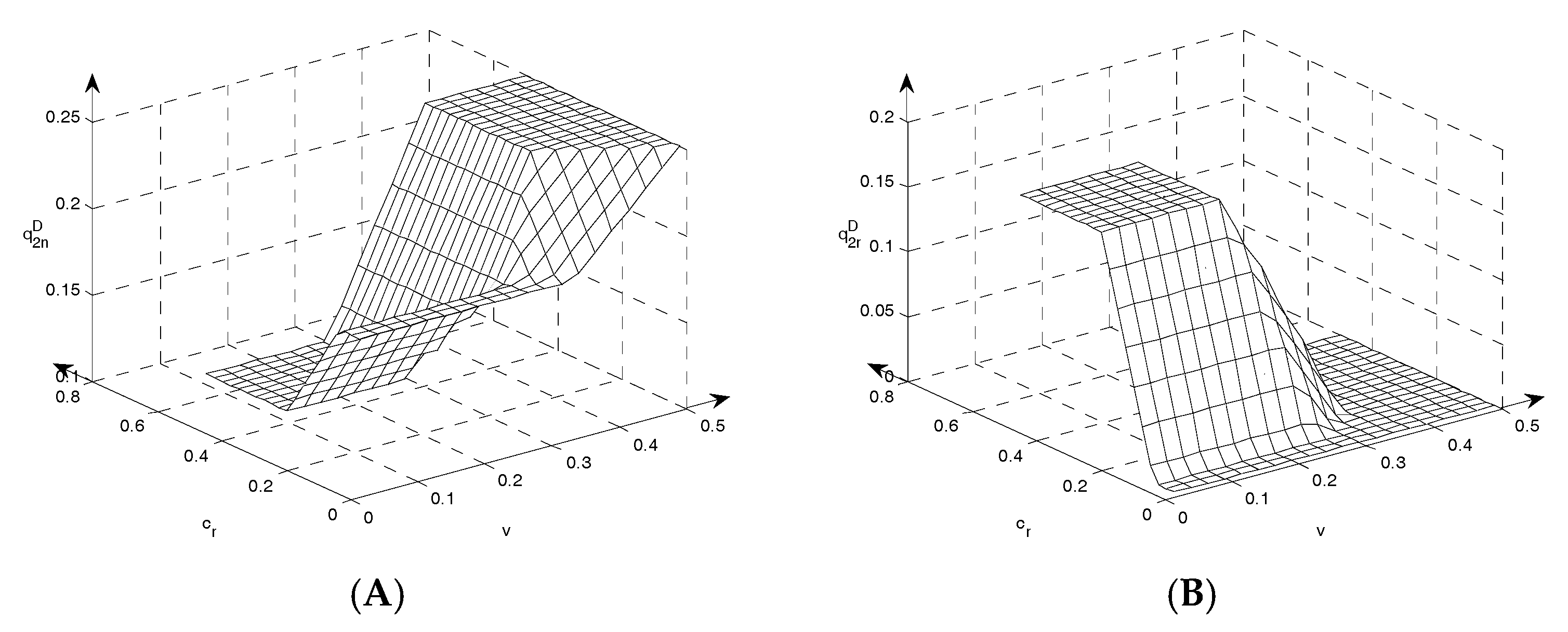
Figure 5A illustrates the impact of parameter ($c_r$, $v$) variation on remanufacturer’s wholesale price in Model D. Figure 5B shows the impact of parameter ($c_r$, $v$) variations on remanufacturer’s quantities in Model D.

Table 5 shows that the wholesale price of remanufactured products increases with the rising cost of new products if the manufacturer purchases remanufactured products. Given that the manufacturer only sells new products or the remanufacturer sells remanufactured products directly, there is no optimal wholesale price for remanufactured products, which is not be affected by $c_n$. However, there is replacement effect between remanufactured and new products sold by manufacturer. When the cost of new products rises, the manufacturer reduces the output of new products and increases sale of remanufactured products, leading to the growing importance of remanufactured products. Therefore, the remanufacturer increases the wholesale price of remanufactured products.

The rising cost of remanufactured products only affects the wholesale price within the ranges of Strategies D-d and D-f. In these two ranges, the remanufacturer resells remanufactured products through the manufacturer, and they do not achieve their maximal output, and thus the wholesale price is correlated with remanufacturing cost and there is collaboration between the manufacturer and remanufacturer. With the rising remanufacturing cost, the manufacturer and remanufacturer share their decreased profits and hence the wholesale prices go up.

When the remanufacturer sells remanufactured products, their selling costs vary, which can affect the wholesale price within the range of Strategy D-e. This is because the wholesale price depends on the competition between remanufactured products resold by the remanufacturer to the manufacturer and the new products made by the manufacturer. The selling cost is correlated with the remanufactured products sold by the remanufacturer. Conversely, the output of remanufactured products is maximal within the range of Strategy D-e. With the rising selling cost, the remanufacturer tends to reduce the quantity of remanufactured products sold directly, and resell them to the manufacturer. Therefore, the manufacturer agrees to purchase more remanufactured products from the remanufacturer with falling wholesale prices.

The rising recycling affects the wholesale prices when the quantity of remanufactured products is maximal and the manufacturer sells remanufactured products, and now the remanufacturer can produce more remanufactured products. When the wholesale price decreases, it can attract manufacturers to purchase more remanufactured products to increase their own profits. Therefore, wholesale prices decline with the rising recycling rate within the ranges of Strategies D-e and D-g.

The quantity of remanufactured products sold by the remanufacturer directly can be influenced by the cost of new products within the ranges of Strategies D-b, D-c and D-e. The manufacturer competes with the remanufacturer completely. With the rising cost of new products, the output of new products declines while that of remanufactured products increases. However, the quantity of remanufactured products is maximal within the ranges of Strategies D-c and D-e. The output of new products in the first period drops with the rising cost of new products. Therefore, the maximal quantity of remanufactured products declines, leading to a decline in quantity of remanufactured products sold by the remanufacturer directly.

$q_{2i}^D$ decreases with the rising remanufacturing cost within the ranges of strategies D-b and D-d, because the output of remanufactured products is not maximal in these two ranges. The remanufacturer adjusts the output of remanufactured products based on the cost variations of remanufactured products.

Similar to the impact of remanufacturing cost on $q_{2i}^D$, the rising selling cost produces the marginal profits of remanufactured products sold by the remanufacturer, dropping within the ranges of Strategies D-b and D-d, and thus the quantity of remanufactured products sold by the remanufacturer is reduced. However, different from the impact $v$ of on $q_{2i}^D$, $q_{2i}^D$ decreases with the increasing range of Strategy D-e. The reason is that the cost increases regardless of reselling or selling directly, with the rising remanufacturing cost, and thus the proportion of remanufactured products of reselling and selling directly is not affected. Conversely, the cost of selling remanufactured products by the remanufacturer increases with the rising selling cost, and thus remanufacturers reduce the quantity of remanufactured products sold by remanufacturers directly.

When the quantity of remanufactured products is maximal and the quantity of remanufactured products sold by remanufacturers themselves is not 0, the recycling rate has an impact on $q_{2i}^D$. The initial marginal profits are high and are subject only to the remanufacturing rate. Hence, the remanufacturer is bound to increase the output of remanufactured products with the rising recycling rate.

Table 6. The impact of parameter variations on manufacturer’s optimal strategies in Model D.

	${\mathit{q}}_{\mathbf{2}\mathit{n}}^{\mathit{D}\mathit{a}}$	${\mathit{q}}_{\mathbf{2}\mathit{n}}^{\mathit{D}\mathit{b}}$	${\mathit{q}}_{\mathbf{2}\mathit{n}}^{\mathit{D}\mathit{c}}$	${\mathit{q}}_{\mathbf{2}\mathit{n}}^{\mathit{D}\mathit{d}}$	${\mathit{q}}_{\mathbf{2}\mathit{n}}^{\mathit{D}\mathit{e}}$	${\mathit{q}}_{\mathbf{2}\mathit{n}}^{\mathit{D}\mathit{f}}$	${\mathit{q}}_{\mathbf{2}\mathit{n}}^{\mathit{D}\mathit{g}}$
$c_n$	$-$	$-$	$-$	$-$	$-$	$-$	$-$
$v$	$0$	$+$	$0$	$+$	$0$	$+$	$0$
$c_r$	$0$	$+$	$0$	$0$	$-$	$0$	$0$
$\delta$	$0$	$0$	$-$	$0$	$-$	$0$	$-$
	${\mathit{q}}_{\mathbf{2}\mathit{r}}^{\mathit{D}\mathit{a}}$	${\mathit{q}}_{\mathbf{2}\mathit{r}}^{\mathit{D}\mathit{b}}$	${\mathit{q}}_{\mathbf{2}\mathit{r}}^{\mathit{D}\mathit{c}}$	${\mathit{q}}_{\mathbf{2}\mathit{r}}^{\mathit{D}\mathit{d}}$	${\mathit{q}}_{\mathbf{2}\mathit{r}}^{\mathit{D}\mathit{e}}$	${\mathit{q}}_{\mathbf{2}\mathit{r}}^{\mathit{D}\mathit{f}}$	${\mathit{q}}_{\mathbf{2}\mathit{r}}^{\mathit{D}\mathit{g}}$
$c_n$	$0$	$0$	$0$	$+$	$+$	$+$	$-$
$v$	$0$	$0$	$0$	$-$	$0$	$-$	$0$
$c_r$	$0$	$0$	$0$	$+$	$+$	$0$	$0$
$\delta$	$0$	$0$	$0$	$0$	$+$	$0$	$+$

lists the impact of parameter ($c_n$, $c_r$, $v$ and $\delta$) variations on manufacturer’s optimal strategies in Model D.

Figure 6A illustrates the impact of parameter ($c_r$, $v$) variations on manufacturer’s wholesale price in Model D. Figure 6B Shows the impact of parameter ($c_r$, $v$) variations on manufacturer’s quantities in Model D.

The quantity of new products is not zero in any of the Strategies and thus with rising cost of new products, the output of new products $q_{2n}^D$ falls. The quantity of remanufactured products sold by the manufacturer is not zero within the ranges of Strategies D-d, D-e, D-f and D-g, whereas it increases with the rising cost of new products within the ranges of Strategies D-d, D-e and D-f; it declines with the rising cost of new products within the range of Strategy D-g. In general, with the rising cost of new products, the manufacturer reduces the output of new products and increases the wholesale of remanufactured products, leading to the increased quantity of remanufactured products sold by the manufacturer within the ranges of Strategies D-d, D-e and D-f. Conversely, with the rising cost of new products, the quantity of used products for remanufacturing falls, and thus $q_{2r}^D$ does not increase with the rising $c_n$ within the range of Strategy D-g, whereas it declines with the rising $c_n$.

When the output of remanufactured products by the remanufacturer is not 0 or maximal, the rising cost of remanufacturing leads to increase in number of new products. Similarly, if the quantity of remanufactured products sold by the manufacturer is not 0 and the total quantity of remanufactured products is not maximal, $q_{2r}^D$ decreases with the rising $v$, within the ranges of Strategies D-d and D-f. The reason is that the output of remanufactured products does not markedly impact the demand for new products if there are only new products in the market. When there are both new and remanufactured products in the market and the output of remanufactured products is not maximal, the slight increase of remanufacturing cost does not affect the output of remanufactured products by remanufacturers. If the consumer demand does not change, the product pattern in the market is not influenced naturally. As a result, the output of new products increases with the rising cost of remanufacturing within the ranges of the remaining Strategies D-b, D-d and D-f. Conversely, $q_{2r}^D$ is 0 within the range of Strategy D-b, and thus the quantity of remanufactured products sold by the manufacturer declines with the rising cost of remanufacturing within the ranges of Strategies D-d and D-f.

The output of new products increases with the rising cost of selling within the range of Strategy D-b when the selling cost rises, whereas it declines with the rising cost of selling within the range of Strategy D-d–D-e. The quantity of remanufactured products sold by the manufacturer increases with the rising $q_{2r}^D$ within the ranges of strategies D-d and D-e. The manufacturer sells new products and the remanufacturer sells remanufactured products in the market within the range of Strategy D-b. Now, the output of remanufactured products is not maximal, and thus the rising cost of selling results in $q_{2i}^D$’s decrease. Due to the replacement effect, the manufacturer tends to produce more new products to squeeze part of the market for remanufactured products. The total quantity of remanufactured products is maximal within the range of Strategy D-e, remanufacturers reduce the sales of remanufactured products due to the rising cost of selling, and they resell them to manufacturers. Hence, the manufacturer tends to reduce the output of new products and increase sale of remanufactured products. $q_{2i}^D$ diminishes, while $q_{2r}^D$ increases in the range of Strategy D-d. The difference is that the quantity reduced by $q_{2i}^D$ is not equal to the quantity increased by $q_{2r}^D$. In other words, the market where the remanufacturer sells the remanufactured products directly is transferred to remanufactured products sold by the manufacturer with the rising cost of selling, but it does not affect the market of new products. As a result, $q_{2r}^D$ increases with rising $c_r$, whereas $q_{2n}^D$ is not affected by the changing $c_r$ within the range of Strategy D-d.

Table 7. The impact of parameter variations on the manufacturer’s and remanufacturer’s optimal profits in Model D.

	${\mathit{\pi }}_{\mathbf{2}\mathit{M}}^{\mathit{D}\mathit{a}}$	${\mathit{\pi }}_{\mathbf{2}\mathit{M}}^{\mathit{D}\mathit{b}}$	${\mathit{\pi }}_{\mathbf{2}\mathit{M}}^{\mathit{D}\mathit{c}}$	${\mathit{\pi }}_{\mathbf{2}\mathit{M}}^{\mathit{D}\mathit{d}}$	${\mathit{\pi }}_{\mathbf{2}\mathit{M}}^{\mathit{D}\mathit{e}}$	${\mathit{\pi }}_{\mathbf{2}\mathit{M}}^{\mathit{D}\mathit{f}}$	${\mathit{\pi }}_{\mathbf{2}\mathit{M}}^{\mathit{D}\mathit{g}}$
$c_n$	$-$	$-$	$-$	$-$	$-$	$-$	$-$
$\mathrm{v}$	$0$	$+$	$0$	$+$	$0$	$-$	$0$
$c_r$	$0$	$+$	$0$	$+$	$+$	$0$	$0$
$\mathsf{\delta }$	$0$	$0$	$-$	$0$	$-$	$0$	$+$
	${\mathit{\pi }}_{\mathbf{2}\mathit{R}}^{\mathit{D}\mathit{a}}$	${\mathit{\pi }}_{\mathbf{2}\mathit{R}}^{\mathit{D}\mathit{b}}$	${\mathit{\pi }}_{\mathbf{2}\mathit{R}}^{\mathit{D}\mathit{c}}$	${\mathit{\pi }}_{\mathbf{2}\mathit{R}}^{\mathit{D}\mathit{d}}$	${\mathit{\pi }}_{\mathbf{2}\mathit{R}}^{\mathit{D}\mathit{e}}$	${\mathit{\pi }}_{\mathbf{2}\mathit{R}}^{\mathit{D}\mathit{f}}$	${\mathit{\pi }}_{\mathbf{2}\mathit{R}}^{\mathit{D}\mathit{g}}$
$c_n$	$0$	$+$	$-$	$+$	$-$	$+$	$-$
$\mathrm{v}$	$0$	$-$	$-$	$-$	$-$	$-$	$-$
$c_r$	$0$	$-$	$-$	$-$	$-$	$0$	$0$
$\mathsf{\delta }$	$0$	$0$	$+$	$0$	$+$	$0$	$+$

lists the impact of parameter ($c_n$, $c_r$, $v$ and $\delta$) variations on manufacturer’s and remanufacturer’s optimal profits in Model D.

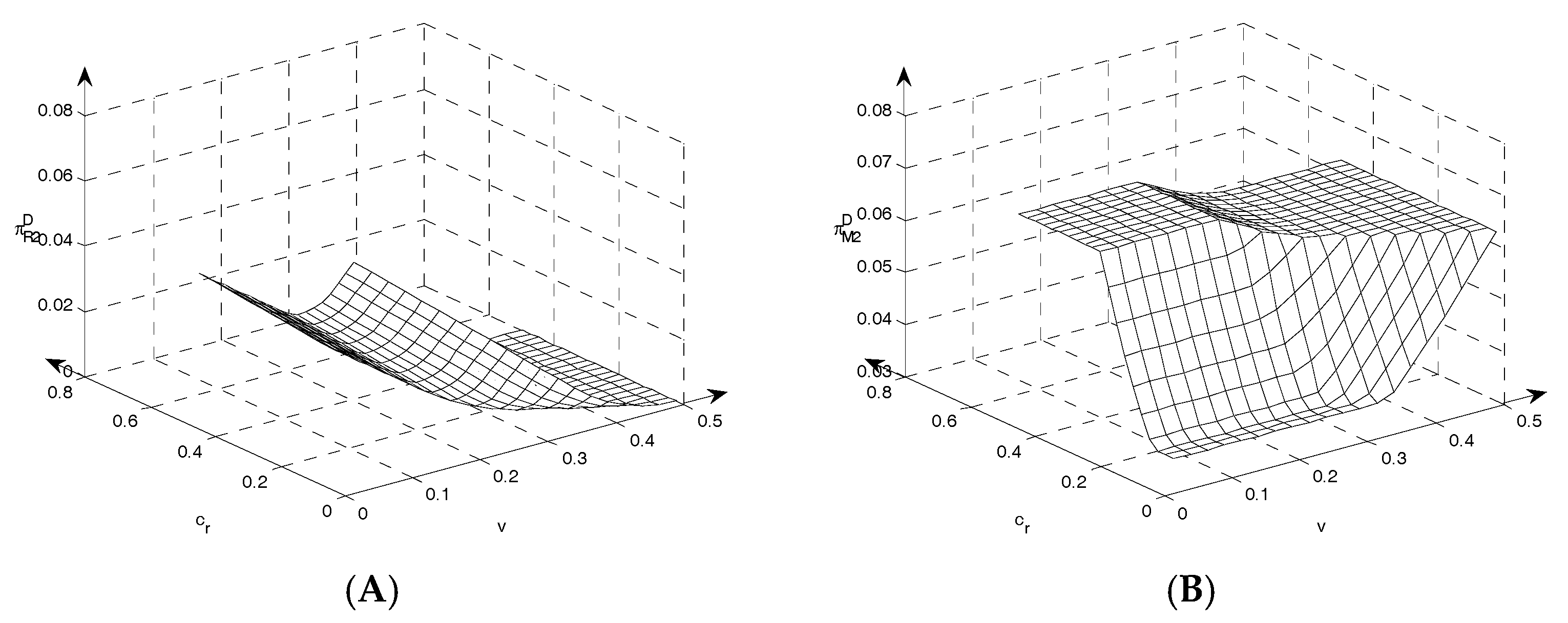
Figure 7A illustrates the impact of parameter ($c_r$,$v$) variations on remanufacturer’s profits in Model D. Figure 7B Shows the impact of parameter ($c_r$,$v$) variations on manufacturer’s profits in Model D.

It is clear in Table 7 that the manufacturer’s profits drop if the cost of new products goes up, but remanufacturer’s profits decline when remanufactured products reach the maximal value. The remanufacturer’s profits increase when remanufactured products are not 0 and do not reach the maximal value. New and remanufactured products are competitive. With the rising cost of new products, the quantity of new products drops. Therefore, the remanufacturer increases the recycling of used products and produces more remanufactured products. The manufacturer’s profits do not grow within the ranges of Strategies D-b, D-d and D-f. When remanufacturers recycle the maximal quantity of used products, they can gain more profits by making more remanufactured products, but remanufacturers’ profits decline with rising ${\mathrm{c}}_{\mathrm{n}}$ within the ranges of Strategies D-c, D-e and D-g without more used products being available.

With the rising remanufacturing cost, the remanufacturer’s profits tend to diminish except in the range of Strategy D-a where remanufactured products are not made. The manufacturer’s profits increase within the ranges of Strategies D-b and D-d, but decrease within the range of Strategy D-f. With the rising remanufacturing cost, the total quantity of remanufactured products from remanufacturer declines or remains constant, whereas the marginal profits decrease, and therefore remanufacturer’s profits always drop. The manufacturer competes with the remanufacturer within the ranges of Strategies D-b and D-d, and thus the remanufacturer’s competitiveness declines while the manufacturer’s competitiveness increases with the rising remanufacturing cost, resulting in the manufacturer’s increased profits. The manufacturer collaborates with the remanufacturer in production and selling activities within the range of Strategy D-f, and the remanufacturer and manufacturer share the decreased profits due to the rising remanufacturing cost.

With the rising selling cost, the profits tend to drop if the remanufacturer sells remanufactured products by himself. It is more sophisticated when the manufacturer is affected by selling costs. Profits are not influenced by the variations of selling costs within the range of Strategy D-c. In the three other ranges where the remanufacturer’s profits decline, profits increase with the rise in cost of selling. The remanufacturer sells all remanufactured products by himself; with the increase in selling cost, the quantity of remanufactured products is fixed, and thus the quantity of new products remains constant. However, the manufacturer’s marginal profit does not change when the remanufacturer’s marginal profit drops. Thus, the manufacturer’s profit does not change but the remanufacturer’ profit declines within the range of Strategy D-c. The remanufactured products sold by the remanufacturer compete with new products, and the remanufactured products resold by the manufacturer in the other three ranges. The rising selling cost reduces the remanufacturer’s competitiveness, and $q_{2i}^D$ decreases, breaking the initial equilibrium. As a result, the remanufacturer’s profits decline with rising $c_r$, whereas the manufacturer’s profits increase with rising $c_r$.

The rise in recycling rate affects the manufacturer’s and remanufacturer’s profits within the ranges of Strategies D-c, D-e and D-g. The remanufacturer’s profits always increase when recycling rate increases, in these ranges. Manufacturers’ profits decline with the rise in recycling rate in the ranges of Strategies D-c and D-e, whereas their profits grow with the rise of recycling rate in the range of Strategy D-g. Manufacturers and remanufacturers collaborate when they sell remanufactured products in the range of Strategy D-g, and manufacturers actively reduce the output of new products and increase the wholesale sales of remanufactured products because they are affected by the high profits of remanufactured products. In other two ranges of Strategies, the remanufacturer sells remanufactured products by himself. With the rising recycling rate, the market of new products will be squeezed, forcing the manufacturer to cut the output of new products. Therefore, the manufacturer’ total profits tend to decline with the rising recycling rate.

6. Contrastive Analyses of Models I and D

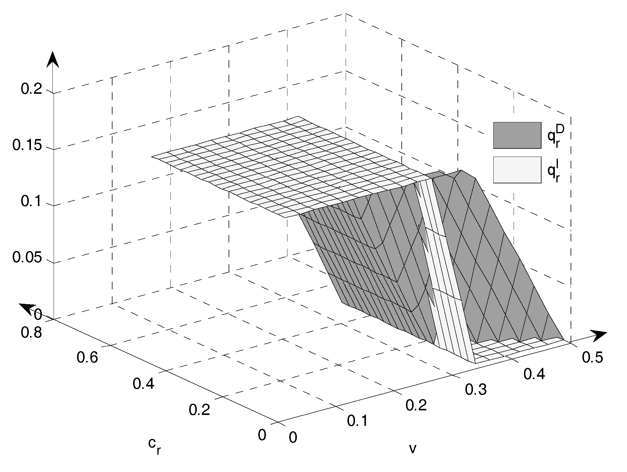
Figure 8 illustrates the comparison of remanufacturing output between Models I and D with the parameter ($c_r$, $v$) variations.

In Figure 8, it is clear that the quantity of remanufactured products is larger in some ranges in Models I and D. When the remanufacturing cost $c_r$ is very high and the selling cost is very low, the quantity of remanufactured products increases in Model D. When the remanufacturing cost is moderate and the selling cost is higher, the quantity of remanufactured products is greater in Model I. This shows that it benefits the production of remanufactured products if the remanufacturer sells them directly. It is the least beneficial for the production of remanufactured products when the remanufacturer resells remanufactured products through manufacturers. When the remanufacturer sells remanufactured products, new and remanufactured products totally compete in the market. The remanufacturers serve as leaders and increases the sales of remanufactured products and reduce the output of new products in order to maximize their own profits. Now, the manufacturer and remanufacturer will not coordinate the quantity of new and remanufactured products for the total profits, leading to the result that the quantity of remanufactured products increases in Model D, the marginal profits of remanufactured products in Model I are greater than those in Model D, and the manufacturer prefers to produce more new products.

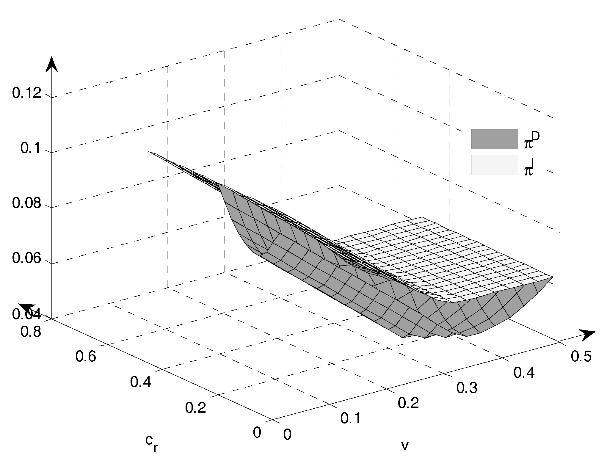
Figure 9 illustrates the comparison of the total profits between Models I and D with the parameter ($c_r$, $v$) variations. It can be seen from Figure 9 that the manufacturer’s and remanufacturer’s total profits in Model I are not always lower than those in Model D, and the total profits are consistent in these two models within the ranges of Strategies D-g and D-a. However, the profits are higher in Model I within other ranges. There is not any output of remanufacturing within the range of D-a. Now, there are not any remanufactured products in these two models, and there are only new products in the market, and the total profits are consistent. The manufacturer resells all the remanufactured products in Model D-g and reaches the maximal value. The manufacturer sells both products in these two models, and, certainly, the quantity of new products is consistent. Therefore, the total marginal profits and sales are consistent, and total profits are bound to be equal.

7. Conclusions

Management of the closed-loop supply chain is a major concern in academia. It is vital to investigate remanufacturing strategies to achieve social, environmental and economic performance in remanufacturing. In light of recycling of products, this article develops a closed-loop supply chain consisting of OEM, remanufacturer and consumer. Consumer willingness to pay for new and remanufactured products varies in mobile phone and automobile markets, and a two-period model of production strategies is developed. The analyses of these two models show that the interaction of strategies in production and selling processes of new and remanufactured products between manufacturers and remanufacturers can exert a marked effect on the economic and environmental performance of remanufacturing. The major findings and implications on management are presented as follows.

The manufacturer’s and remanufacturer’s total profits in Model I are always higher than those in Model D, because their interest is consistent in Model I and there is no resale between them so that the dual margin effects are overcome, leading to the increased efficiency in the supply chain. In addition, regardless of the very low production cost of remanufactured products in Model I, new products are made in the overall supply chain. Conversely, with extremely low marginal profits of remanufactured products, the remanufactured products are not made in the overall supply chain. When the marginal profits of remanufactured products are moderate, both new and remanufactured products are made in the overall supply chain. In addition, with the falling cost of remanufactured products, their output increases.

We summarize a number of general results from the two CLSC models as follows. (1) When remanufacturing costs and selling costs are low, remanufacturers choose to recycle and sell all their remanufactured products and compete with manufacturers completely. (2) When remanufacturing costs are low, with the rising selling costs, remanufacturer chooses to sell part of the remanufactured products directly and resell part of remanufactured products to manufacturers, and hence they compete and collaborate with each other. (3) When remanufacturing costs are low while selling costs are high, the remanufacturer recycles and produces remanufactured products and sells all of them to the manufacturer, and they cooperate completely. (4) When the remanufacturing costs are extremely high, remanufacturers will probably not recycle used products. Parameters such as costs of new products, costs of remanufactured products, selling costs, and recycling rates impact the manufacturer’s and remanufacturer’s profits. With the rising costs of new products, the manufacturer’s profits always diminish, whereas remanufacturer’s profits decrease when the output of remanufactured products is maximal. When the quantity of remanufactured products is not 0 or maximal, their profits step up. With the rising of remanufacturing costs, the remanufacturer’s profits always decline. The manufacturer’s profits grow when competes with remanufacturers and fall when they collaborate. With the rising selling costs, the remanufacturer’s profits decline if he sells remanufactured products directly. It is relatively more complicated when manufacturer are affected by selling costs. When the recycling rate increases, it affects the manufacturer’s and remanufacturer’s profits within the ranges of Strategies D-c, D-e and D-g. In addition, the remanufacturer’s profits increase within the rising recycling rate in these ranges. Remanufacturer’s profits decline with the rising recycling rate within the ranges of Strategies D-c and D-e, while they increase with the rising recycling rate within the range of Strategy D-g.

Our paper investigates the effect of some parameters on the equilibrium solution of the model, and presents some insights for policy makers, such as improving the technology and design level of the manufacturer, reducing the cost of waste disposal and increase the minimum ration of used product to total quantity. In addition, our results can provide some guidance for policy makers. For example, this article offers insights for understanding the relationship between remanufacturer and manufacturer. In this context, they could be of assistance to policy makers in offering incentives, such as reward or punishment, to the businesses that provide remanufactured products.

This study investigates competition and cooperation in closed-loop supply chains by taking remanufacturing mobile phones and automobile components into consideration. It is assumed that remanufacturers serve as leaders in Stackelberg game, different from the previous studies which assume that manufacturers act as leaders in Stackelberg game, from the remanufacturer’s perspective, the gaming relations between the remanufacturer and manufacturer are analyzed, improving the game theory in remanufacturing supply chains. In addition, the model of competition and cooperation in the closed-loop supply chains suits the remanufacturing realities. Therefore, this can provide some scientific guidance for remanufacturers as well as governments which introduce and optimize some relevant rules and regulations.

However, there are some limitations in this study. Firstly, we only consider single remanufacturer and single manufacturer in CLSC. In reality, there are multitude players in the market structure, and it is possible for the manufacturer to sell the new products and the remanufactured products through the retailer. Secondly, we assume the remanufacturer recycles used products and proceeds to remanufacture, without considering technology licensing, while a manufacturer’s production of patented products is protected by the patent law, any the company that intend to remanufacture that product must get the manufacturer’s licensing approval.

The future research can explore the following topics. Firstly, it is assumed that the remanufacturer recycle used products whereas in the future the manufacturer may recycle and serve as the Stackelberg leader. In this assumption, the manufacturer competes and collaborates with the remanufacturer (recycling competition, recycling collaboration, selling competition and selling collaboration). Secondly, due to the low selling cost, the remanufacturer does not provide products for manufacturers. Thus, we can examine how manufacturers collaborate with remanufacturers through contracts or restrict the manufacturer’s competitiveness in markets. Finally, it is assumed that prices affect consumer willingness to pay for remanufactured products and we may consider other factors such as government subsidies, the quality of recycled products, the quality and design of new remanufactured products and the impact of services on the collaboration and competition between manufacturers and remanufacturers.