Article

Assessment of the Air Pollution Level in the City of Rome (Italy)

by
Gabriele Battista
*,
Tiziano Pagliaroli
,
Luca Mauri
,
Carmine Basilicata
and
Roberto De Lieto Vollaro
Department of Engineering, University of Roma TRE, via della Vasca Navale 79, Rome 00146, Italy
*
Author to whom correspondence should be addressed.
Sustainability 2016, 8(9), 838; https://doi.org/10.3390/su8090838
Submission received: 20 May 2016 / Revised: 17 August 2016 / Accepted: 19 August 2016 / Published: 23 August 2016

Abstract

:
Exposure to pollutants is usually higher in cities than in the countryside. Generally, in the urban areas pollution sources as traffic, power generator and domestic heating system are more intense and spatially distributed. The pollutants can be classified as a function of long-term toxicological effects due to an exposure and inhalation. In the present work, several kinds of pollutants concentration generated in Rome during 2015 have been analyzed applying different advanced post-processing technique. In particular, statistic and cross-statistic have been computed in time and phase space domain. As main result, it is observed, as expected, that all the pollutant concentrations increase during the winter season into a couple of time ranges despite of [O3] that has high values in summer. It can be clearly concluded that Rome has a strongly unsteady behaviour in terms of a family of pollutant concentration, which fluctuate significantly. It is worth noticing that there is a strong linear dependence between [C6H6] and [NO] and a more complex interdependence of [O3] and [C6H6]. Qualitatively is provided that, to a reduction of [C6H6] under a certain threshold level corresponds an increase of [O3].

1. Introduction

Outdoor air pollution has myriad sources, both natural and anthropogenic. It is a mixture of mixtures, and the mix of contaminants in outdoor air varies widely in space and time, reflecting variation in its sources, weather, atmospheric transformations and other factors. In any particular place, the pollution in outdoor air comes not only from local sources, but also from sources that affect air quality regionally and even globally [1]. The main reason for the air quality problems is urban population growth, because people are constantly moving from rural to urban areas [2]. The air pollutants result higher in urban area because of a combination of many elements such as industrial activities, energy production plants and domestic heating [3]. They are noticeable by the toxicological effects resulting from long-term exposure via inhalation [4].
The major pollutants produced are related to human activities, especially those produced by combustion and industrial processes. The International Agency for Research on Cancer (IARC) focused the attention on the human exposures to PM (Particulate Matter). The risk of being exposed to a mixture of pollutants depends on particulate matter smaller than 2.5 μm, which is a common useful indicator [4]. Therefore, the PM2.5 can be taken as indicator of population exposure to outdoor air pollution. In 2010, 3.2 million of people died because of cardiovascular disease, caused by the exposure to ambient fine particles (PM2.5) and 22,300 people died because of lung cancer. China and East Asia show the largest number of people who lost their life [5,6].
With reference to NO2, SO2 and (PMs) there is general agreement in the scientific literature that they are the main agents responsible for the damage encountered on monuments and historical buildings in urban areas [7]. Atmospheric composition is of unquestionable importance in the study of the damage produced on building materials of artistic interest, since it directly influences the species characteristics and entity of the degradation mechanism occurring on the cultural heritage.
The urban areas modified the environmental features that contributed to the increase of pollution. As a matter of fact, the large concentration of the built environment, road pavement and the high building materials capacitance changed the local micrometeorological conditions. Air temperature, humidity and wind velocity and direction are altered in the urban environment compared to rural areas. Furthermore, road traffic, domestic heating, industrial activities and lack buildings energy performance involves high discomfort for users [8,9,10,11,12,13,14,15,16,17,18,19,20]. Besides the increase of pollutions, urbanization has led to an increase of the urban heat island intensity (spatially-averaged surface or air-temperature difference between an urban and surrounding rural area(s) [21]). Several studies are focused to reduce the urban heat island effect with different mitigation techniques [22,23,24,25,26,27,28].
The people exposed to air pollutants are even more evident considering the weak ventilation, because of the presence of high buildings with a consequent reduction of the dispersion of air masses. For this reason, the contaminants formed below the building height remain at the pedestrian level and increase the health damages especially during thermal inversion episodes. Several studies were conducted to analyse the correlation between the street canyon features and the pollution dispersion [29]. If the ratio between the average height of the buildings (H) and the width of the canyon (W) is high enough to establish skimming flow conditions (at least higher than 0.65), the retention of pollutants within the urban canopy layer will be amplified [30]. The major street canyons in the cities have high value of the ratio H/W with a consequent established helical vortex with an axis parallel to the canyon direction. In this case, the pollutants that go out of the canyon are reduced [31].
The identification of analysis tools and methods, pollutant concentrations measurement, comparison with the threshold values prescribed by law, are the activities foreseen by the legislations in order to monitor the air quality and predict rehabilitation through the definition of plans of interventions.
As a first step, in order to plain a control strategy of the pollution concentration in medium and high scale cities, proper measurement and data processing are required to highlight the achievement of dangerous concentration levels of pollutants and formulate a prediction model.
Actually, the main active control strategy is based on the introduction of some limits of the urban traffic (e.g., number of the vehicles and vehicle categories that are authorized to transit). Other interventions include the increase of efficiency of the heating systems in buildings such as the replacement of traditional boilers with condensation ones integrated with more performing regulation systems based on energy load tracking.
In the present work, several kinds of pollutants concentration such as [CO], [SO2], [NOx], [NO], [NO2], [C6H6], [PM10], [PM2.5] and [O3] generated in Rome during 2015 have been analysed. These pollutants were taken from the Directive 2008/50/EC, the main legislation about ambient air quality. In these analyses we applied different advanced post-processing techniques. Statistic and cross-statistic have been computed in time and Fourier domain. In particular, probability distribution, Kurtosis, Skewness, Poincaré sections and cross-correlation of the different pollutants were analysed in order to assess the air pollution level in the city of Rome and the correlation of anthropogenic sources with the pollutant emission. The extreme value theory was applied to the experimental data. Especially using the generalized extreme value (GEV) distribution, several fittings of the experiment probability density functions were calculated. GEV distribution introduced by Fisher and Tippett [32] is commonly applied in environmental science to model a wide variety of natural extremes, including floods, rainfall, wind speeds, wave height, snow depths, earthquake, and other maxima. For the present research activity, probability density functions fitting of the pollutant concentration were calculated. The GEV distribution turned out to be very attractive mathematical tool since its inverse has an analytical form, and its parameters are can be easily estimated [33,34,35,36,37,38]. This last feature allows us to compute the return period: the likelihood of an event to occur. This post-processing strategy is common applied to pollution database to develop model. Shen et al. developed a statistical model using extreme value theory to estimate changes in ozone episodes [39].

2. Materials and Methods

2.1. Characteristics of the Study Area

Rome is the capital of Italy, and the largest city situated in the west-central part of the country. It is also one of the most populous cities in the European Union with 2.9 million residents in 1285 km2. Considering the metropolitan area of Rome, the population reaches up to 4.3 million residents in 5352 km2. With a history of more than two and half thousand years, Rome is called the Eternal City because of the number of open-air museums. It is a mixture of a modern city and a plethora of monuments, piazzas, villas, museums, churches, Egyptian obelisks, the Forum and Vatican City. Its climate is typically Mediterranean: winters are cool and humid and summers are hot and dry. In the coldest month (January) the temperature can reach about 0 °C, and in the warmest months (July and August) the temperature can reach 36 °C.
The problem has two faces: there are a lot of pollutant activities and the public transport is not efficient enough to reduce the number of cars. Pedestrian and public transport are only 20% of the total mobility, while 60% of journeys are made by private means of transport; in the historical centre this modal share changes into 34% of pedestrians, 29% of public transport and 37% of private transport [40]. In order to partially solve the problem of pollution, the Government has developed a lot of policies to improve the net of the means of transport [41].
Studying the air pollutant in the city of Rome is important because there is a high density of population and for the effects of pollutant on the variety of open-air museum.

2.2. Pollutant Legislation

The European Union policy on air quality has the goal of implementing appropriate instruments aimed at improving air quality. The control of emissions from mobile sources, improving fuel quality and promoting and integrating environmental protection requirements into the transport and energy sector are the main goals of this policy [42].
The Directive 2008/50/EC of the European Parliament [43] is the main legislation about ambient air quality. It fixes health based standards and objectives for a number of pollutants in air. These standards are applied in different time spans because the observed health impacts associated with the various pollutants occur over different exposure times. Table 1 shows the standard adopted in the Directive 2008/50/EC.

2.3. Post Processing Techniques

In this paper, different statistics and cross-statistics have been computed in time and Fourier domain. These correspond to time-frequency analysis that study a signal in both the time and the frequency domain simultaneously. In particular, the different techniques adopted are:
  • Probability distribution describes the possible values that a random variable can take within a given range.
  • Kurtosis is a measure of whether the data have a flattening or elongation from the normal distribution. High kurtosis indicates a flattering distribution, while low values indicate an elongation distribution.
  • Skewness is a measure of the asymmetry of the distribution. A data set is symmetric if it looks the same to the left and right of the center point.
  • Poincaré sections are a way to represent a dynamical system. The surface of section presents a trajectory in n-dimensional phase space in an (n-1)-dimensional space. By picking one phase element constant and plotting the values of the other elements each time the selected element has the desired value, an intersection surface is obtained. The phase space is a surface that describes all the possible states of a system.
  • Cross-correlation is a measure of similarity of two data series as a function of the lag of one relative to the other.
  • Coefficient of variation normalizes the standard deviation with the mean of a data. This index gives information about the variability of a data set.
  • Generalized Extreme Value distribution is often applied to analyse a large set of data characterized by small or large value. In this approach three simpler distributions into a single form are combined, allowing a continuous range of possible shapes.

2.4. Monitoring Station Network

ARPA Lazio [44], the regional environmental agency, operates several air quality monitoring sites in the Lazio Region, including Rome. The Rome monitoring network consists of 10 monitoring stations of [CO], [SO2], [NOx], [NO], [NO2], [C6H6], [PM10], [PM2.5] and [O3] that are shown in Figure 1. The monitoring network acquires concentration data every hour and every stations is set to monitor different type of concentrations. All the stations taken into account are placed inside high density urban areas that are characterized by traffic and domestic heating system pollutant sources.
The monitoring stations are constituted by fixed structures in which the entire measurement instrument, the acquisition systems and local storage are placed inside. The procedures and the control of the quality of the measures are assured by ARPA Lazio [45]. A zero value was considered when an instruments errors were found.
All the measurement instruments are made by Project Automation. Table 2 shows the sensors used for each concentration.

3. Results and Discussion

In the present study, the data recorded in 2015 were considered. It is useful to consider the mean values of contaminants of each station in order to represent the average pollutant concentrations of Rome.
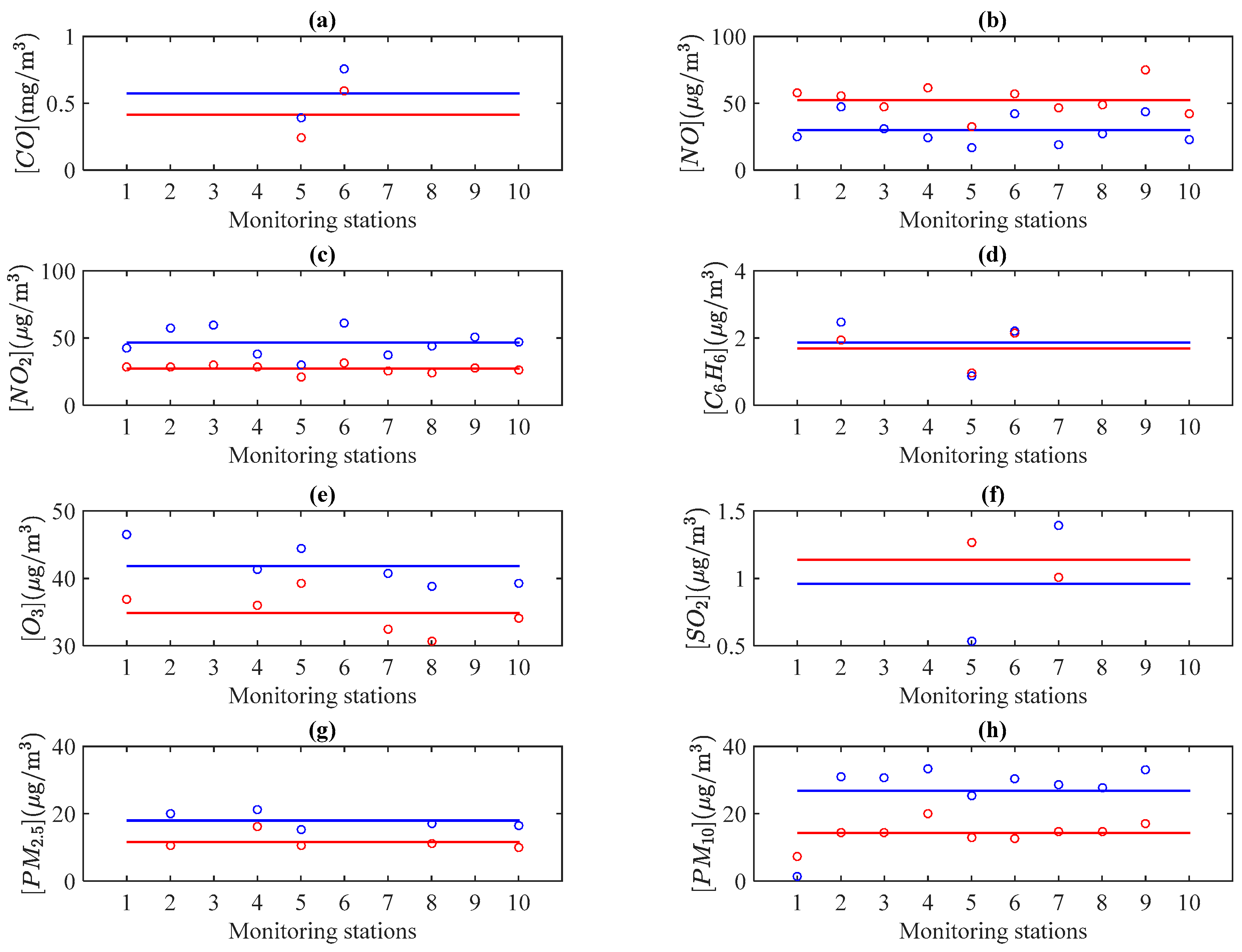
Before calculating the mean values concentrations of Rome, Figure 2 and Figure 3 show the mean, standard deviation, Kurtosis and Skewness values of each pollutant during the year 2015. These are analysed in order to find the behaviour of each pollutant in the different stations. In the case of [PM10], there is only one station that indicates a different Kurtosis value than the others. Despite this consideration, in all the concentrations the Kurtosis and Skewness values of the different stations are similar and it suggest that the mean of the network is possible.
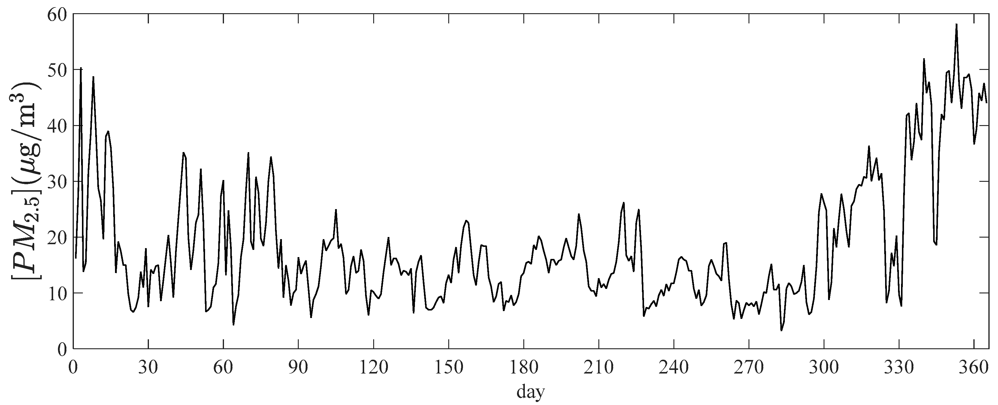
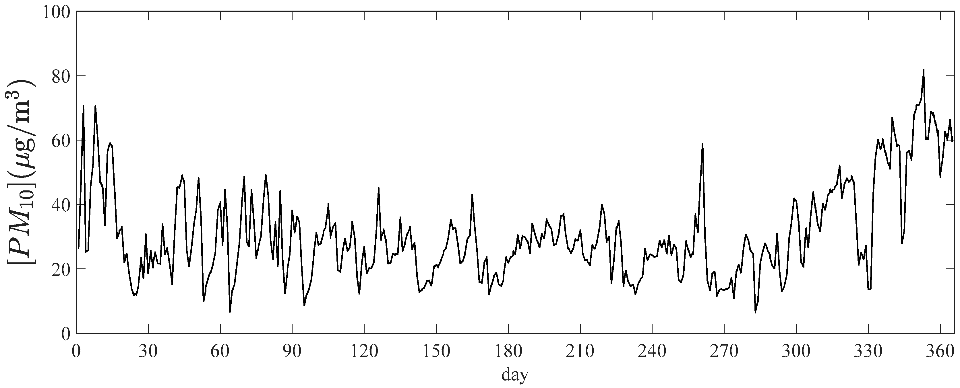
From Figure 4, Figure 5, Figure 6, Figure 7, Figure 8, Figure 9, Figure 10 and Figure 11 is shown how the mean concentration of all stations work during the year in each hour. It can been seen that the major pollutant concentrations happen in the winter seasons from 8 to 13, and from 17 to 2, when there is a greater flow of cars in the city. The highest values are recorded from 19 to 23, when the heating systems are turned on. During the night there are lower values due to the turned off heating systems that is usually in Italy. In the summer, the high values in these hours are due to the urban traffic.
It is worth noticing that the [CO], [NO], [NO2] and [C6H6] have similar trend during the year suggesting the presence of pollutant source simultaneously.
The [O3] is recorded to be higher in the summer and during the hottest hours, when the solar radiation is highest. As a matter of fact, the presence of solar radiation allows the reaction of nitrogen dioxide (NO2) in the formation of ozone (O3).
The [SO2] have values up to 8 µg/m3 compared with the limit of 125 µg/m3 reported in Table 1. That is foreseeable because the [SO2] is mainly caused by the combustion of fuel at power plants and other industrial facilities. As a matter of fact, in the center of Rome there is not this kind of system.
The concentration of PM2.5 and PM10 has high values in the winter season and reach the maximum values in the last two months of 2015, with values close to 50 µg/m3 of PM2.5 and values close to 70 µg/m3 of PM10.
The main pollutant species in terms of probability density function (pdf) have been analysed and represented in normalized form in order to have zero mean and unitary standard deviation defined as follows:
x n o r m = x x σ x
where as is denoted the ensemble average and as σ is indicated the standard deviation.
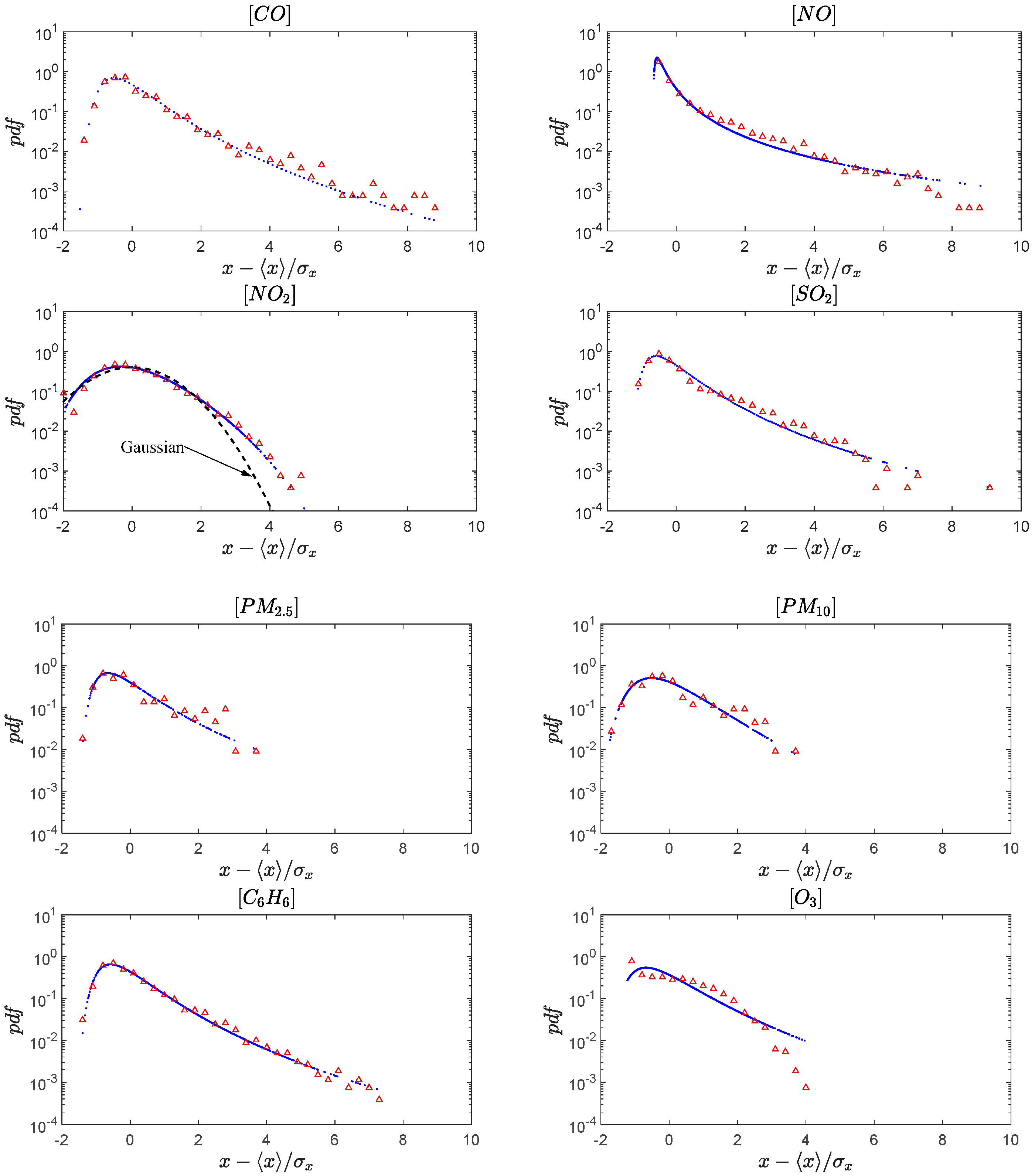
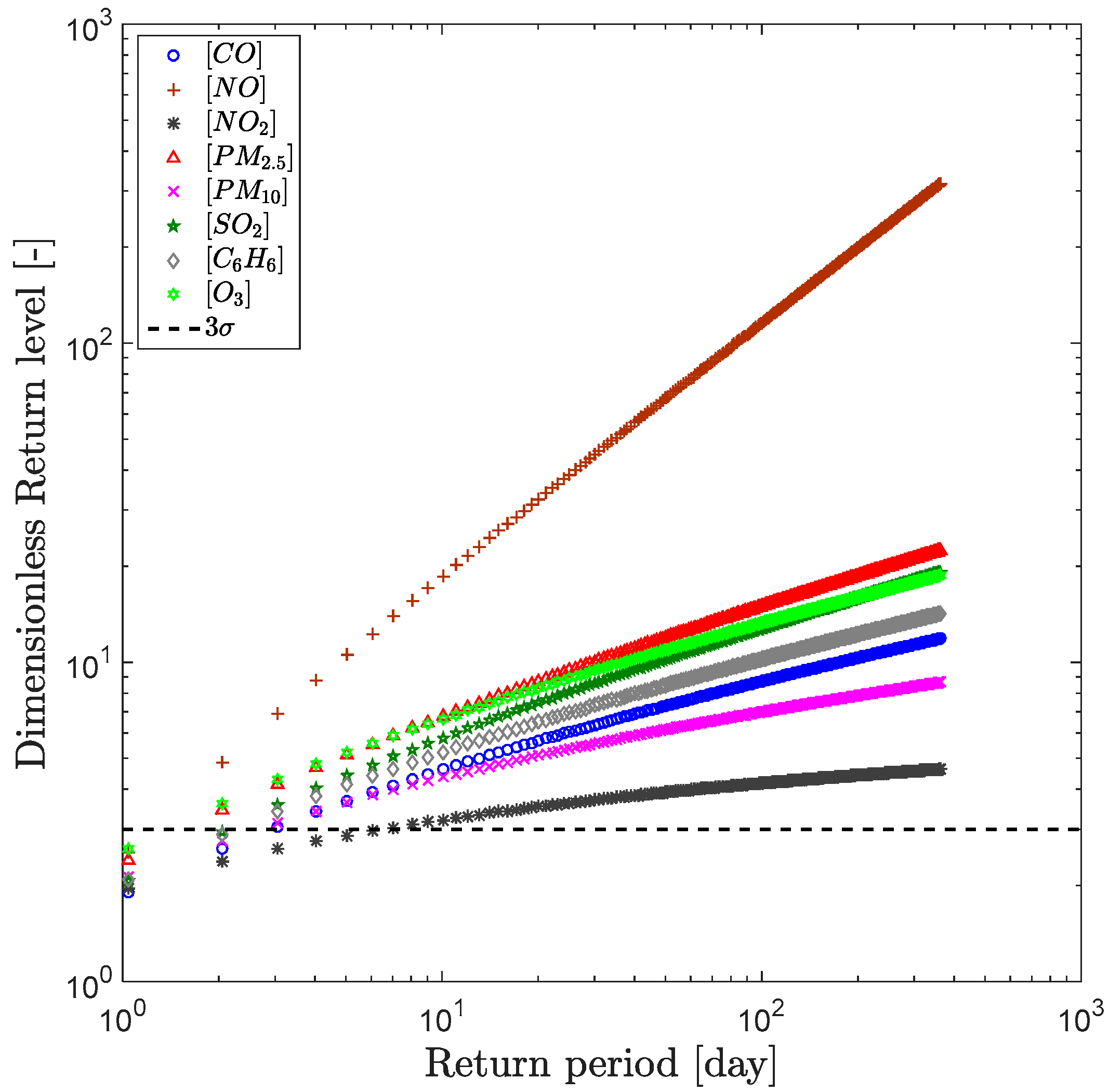
It is shown in Figure 12 that [CO], [NO], [SO2] and [C6H6] have a narrow distribution around the most frequent value and significant positive tail. The latter aspect can be ascribed to intermittent energetic events embedded in concentration time histories. To better clarify this aspect all pdf are fitted using the Generalized Extreme Value (GEV) function. By means of the GEV function, the return level and period were calculated in order to evaluate the occurrence time of these events as reported in Figure 13. With reference to the return period of [NO], every two days a high energetic peak in [NO] concentration can be detected. On the other hand, in [NO2] time history intermittent events are rarely observed. This aspect is a footprint of chaotic behavior of the Rome in terms of pollutant generation and could be taken into account during the modelling stage of this process.
Instead [NO2], [PM2.5], [PM10] and [O3] have a distribution with a more flat trend. In particular, [NO2] pdf is well fitted by the Gaussian pdf except for a small region over 3σ where a departure of the positive tail can be clearly observed. In the latter case, we can consider, in a first approximation, equally probable concentrations in a certain range.
Analysing the probability distributions in comparing with the standards reported in Table 1, it could be notice that [NO2], [PM2.5], [PM10], [C6H6] and [O3] exceeds the limit of legislation during the year. In particular, 64% of time the [NO2] was over the limit of 40 µg/m3, 23% of time the [PM2.5] was over the limit of 25 µg/m3, and 21% of time [PM10] was over the limit of 40 µg/m3. Regarding the concentration of [C6H6] and [O3] the time in which the concentration is over the limit of legislation is less than previous pollutant: 4% of time the [C6H6] was over the limit of 40 µg/m3 and 3% of time the [O3] was over the limit of 120 µg/m3.
In 2015, regarding the limit in the short averaging period (from 1 to 24 h), [NO2], [SO2] and [CO] haven’t exceeded the legislation thresholds. For [PM10] the limit of 50 µg/m3 for an averaging period of 24 h was exceeded 39 times that is more than 35 permitted exceedances each year by the legislation. These exceedances are concentrated in December when there was a combination of exogenous state variable (i.e., temperature, humidity and wind velocity and direction, and traffic flow) and low rainfall. For [O3] the limit of 120 µg/m3 for an averaging period of 8 h was exceeded 7 times. For this concentration, the legislation permitted 25 exceedances days over 3 years.
As stated previously and as further confirmed by the values assumed by Kurtosis and Skewness (see Table 3), with reference to the set of [CO], [NO], [SO2] and [C6H6] a high Kurtosis value is evaluated, indicating that these pollutants are present on Rome in constant quantities. On the other hand the high Kurtosis values suggests a sharped distribution around the mode. Whereas the coefficient of variation of [NO] have large value indicating that there are high energetic extreme value (see Figure 12).
In the case of [NO2] the values assumed by the Kurtosis are close to those of a Gaussian distribution as confirmed by the comparison in Figure 12, indicating the presence of a species of pollutant that fluctuate significantly around an average value.
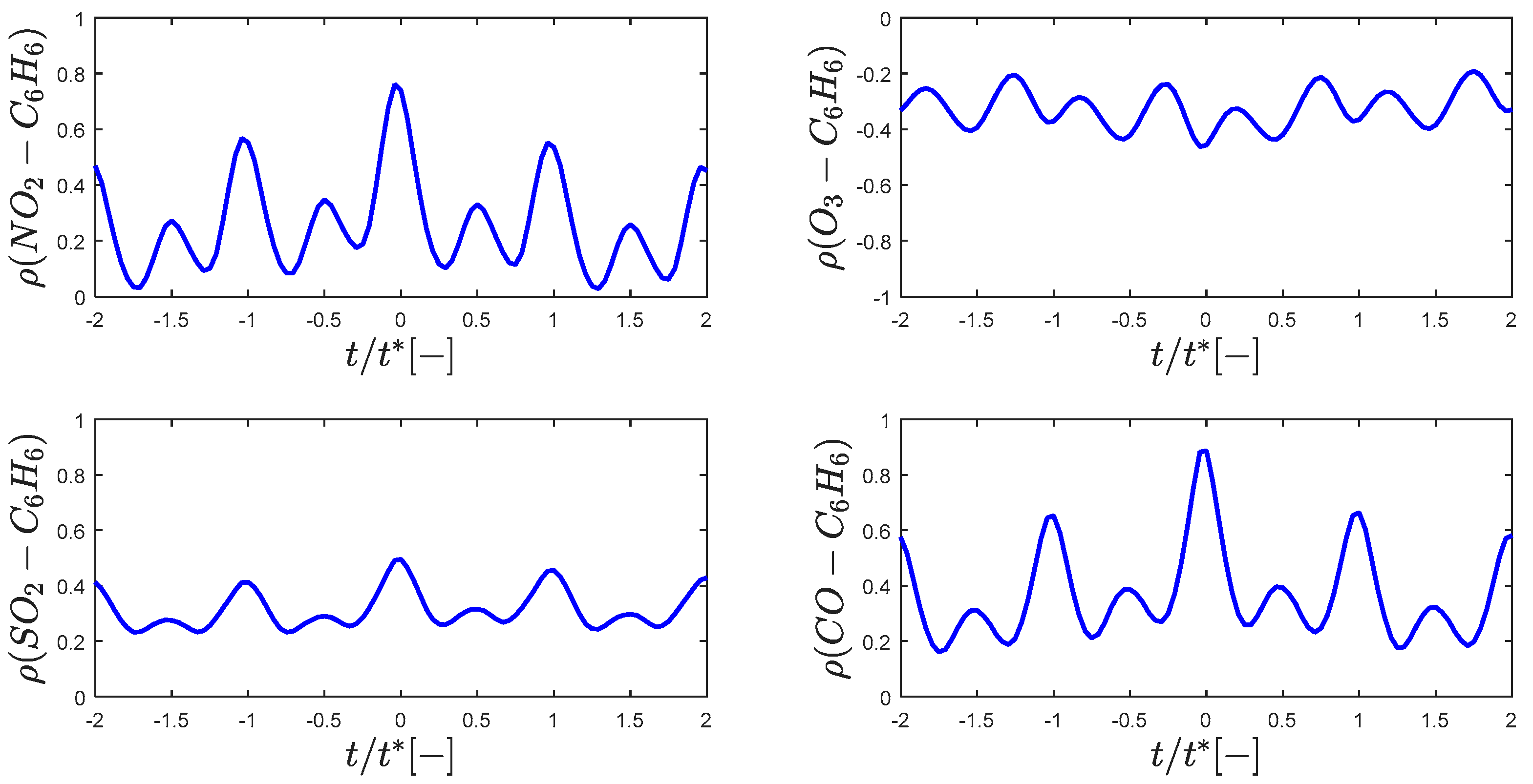
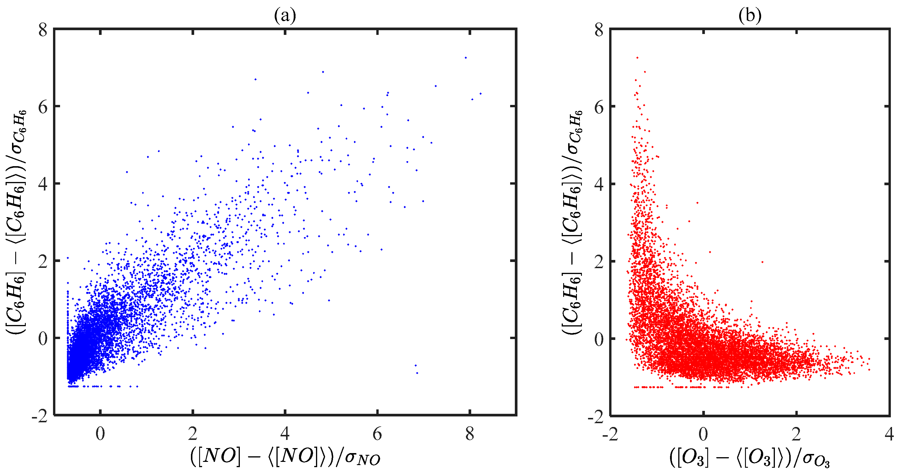
Given that the most important benzene source is the urban traffic, the concentration of benzene may be used as an index of city traffic flux and its time history can be taken into account as reference. The production of benzene is characterized by small oscillations in Rome during the time window investigated. Furthermore, [C6H6] are strongly related to the concentration of pollutants species such as [CO], [NO] and [NO2], as confirmed by the cross-correlation values reported in Figure 14. This correlation is due to the fact that nitrogen oxide and carbon oxides are combustion products and that their fluctuations are due to the oscillations of the city traffic flux. It is noteworthy that [O3] is weakly related to the production of benzene but it is indeed in phase opposition with it. To further investigate this interesting aspect, the Poincaré section of [C6H6] upon [NO] and [C6H6] upon [O3] are represented in Figure 15. As noted above there is a strong linear dependence between [C6H6] and [NO] and a more complex interdependence of [O3] and [C6H6]. More specifically an inverse proportionality is clearly observed as formalized in the following:
| d [ C 6 H 6 ] d t | ~ | d [ O 3 ] d t |
Qualitatively is provided that to a reduction of [C6H6] under a certain threshold level corresponds an increase of [O3]. Such behaviour could be attributed to exogenous state variable, which were not taken into account in the present work.

4. Conclusions

Observance of air quality standards represents a great challenge in cities, especially in the ones in which traffic and other additional sources are combined with bad weather conditions. With reference to this issue, the results herein provided shown that the major pollutant concentrations are observed in the winter seasons during the intense traffic flow and the threshold values are often exceeded. Furthermore, according to the coefficient of variation values, Rome has a strongly unsteady behaviour in terms of a family of pollutant concentration which fluctuate significantly.
[C6H6] are strongly related to the concentration of pollutants species such as [CO], [NO] and [NO2], as confirmed by the cross-correlation analysis. This correlation is due to the fact that nitrogen oxide prompts and carbon oxides are combustion products and that their fluctuations are caused by the oscillations of the city traffic flux. [O3] is weakly related to the production of benzene and it is also in phase opposition with it. For this reason, the Poincaré section of [C6H6] upon [NO] and [C6H6] upon [O3] was investigated. It is worth noticing that there is a strong linear dependence between [C6H6] and [NO] and a more complex interdependence of [O3] and [C6H6]. Qualitatively is provided that, to a reduction of [C6H6] under a certain threshold level which corresponds to an increase of [O3]. Such behaviour could be attributed to exogenous state variable.
The main objective for the reduction of air pollutant is to reach, thanks to the implementation of suitable mobility policies, an urban sustainable development, i.e., to improve traffic mobility conditions, to increase road safety and to decrease traffic caused by pollution and to re-qualify urban spaces. It includes rationalizing public space, safeguarding citizens’ health and life quality, and preserving historical and architectural heritage.
The government is promoting both long and short-term activities to reach these goals. From the analysis of the current air situation, it is clear that traffic is the reason why the pollutant concentrations are so high. Traffic is the main source of [CO], [C6H6] and [PM10] concentrations.
In order to reduce the pollution in Italian cities and in particular in Rome, measures are needed to decrease the level of the various substances dispersed into the air. One of the main actions that can be performed is the reduction or elimination of the use of the most polluting cars, i.e., cars Euro 0, 1 and 2. As a matter of fact, Roma Capitale has imposed the circulation reduction of these cars permanently from 15 December 2015 [46].
Regarding the reduction of the pollutants due to buildings heating systems, it is necessary to replace traditional boilers with more efficient systems, such as condensing boilers. As a matter of fact, the condensing boilers allow reducing the utilization of combustion and a consequence decrease of emission.
However, the boilers are only one element of the heating systems. Its efficiency depends on other elements such as distribution, emission and regulation. Using condensing boilers coupled with other high heating systems elements, can improve the total efficiency and reduce the environmental emission.
The Poincaré sections in Figure 15 gives a significant contribution to the modeling purpose: such as dynamical model (ODE) or regression approach (LUR) (see among many [47,48]).
More specifically, the experimental analysis shows a correlation between [C6H6] over [NO] and [C6H6] over [O3]. These aspects are well known for small scale zero-dimensional reactor, but for very large scale problems as the city domain is not commonly investigated. Therefore, a reduction of a three dimensional large scale process to zero-dimensional phenomenon as in homogeneous volume can be consider the first step for a mathematical model development by means of an ODE system as follows:
x ˙ = f [ x ( t ) ]   w h e r e   x ( t ) = { [ NO ] ,   [ O 3 ] ,   [ C 6 H 6 ] , }
This aspect is the fundamental task to predict the time evolution of the pollutant species generated within an urban domain.
Furthermore, as a result, it can be clearly concluded that Rome has a strongly unsteady behaviour in terms of pollutant concentration. All-time series are positive skewed, indicating that some short time rare events, of pollutant concentration, have an order of magnitude bigger than the expected values. Such as intermittent behaviour must be taken into account for modelling purpose.

Acknowledgments

The authors are grateful to ARPA Lazio which provided the experimental data.

Author Contributions

The work was designed by Gabriele Battista, Tiziano Pagliaroli and Roberto De Lieto Vollaro. Gabriele Battista and Tiziano Pagliaroli wrote the paper and perform the statistic and cross-statistic analysis. English corrections were revised by Luca Mauri and Carmine Basilicata. Finally, Roberto De Lieto Vollaro supervised the work related to the paper. All authors read and approved the final manuscript.

Conflicts of Interest

The authors declare no conflict of interest.

References

  1. International Agency for Research on Cancer (IARC). Outdoor air pollution. In IARC Monograph on the Evaluation of Carcinogenic Risks to Humans; International Agency for Research on Cancer: Lyon, France, 2015; Volume 109. [Google Scholar]
  2. Mayer, H. Air pollution in cities. Atmos. Environ. 1999, 33, 4029–4037. [Google Scholar] [CrossRef]
  3. Guerrieri, M.; Corriere, F.; Rizzo, G.; Casto, B.L.; Scaccianoce, G. Improving the Sustainability of Transportation: Environmental and Functional Benefits of Right Turn by-Pass Lanes at Roundabouts. Sustainability 2015, 7, 5838–5856. [Google Scholar] [CrossRef] [Green Version]
  4. Schiavon, M.; Redivo, M.; Antonacci, G.; Rada, E.C.; Ragazzi, M.; Zardi, D.; Giovannini, L. Assessing the air quality impact of nitrogen oxides and benzene from road traffic and domestic heating and the associated cancer risk in an urban area of Verona (Italy). Atmos. Environ. 2015, 120, 234–243. [Google Scholar] [CrossRef]
  5. Lim, S.S.; Vos, T.; Flaxman, A.D.; Danaei, G.; Shibuya, K.; Adair-Rohani, H.; Adair-Rohani, H.; Amann, M.; Anderson, H.R.; Andrews, K.G.; et al. A comparative risk assessment of burden of disease and injury attributable to 67 risk factors and risk factor clusters in 21 regions, 1990–2010: A systematic analysis for the Global Burden of Disease Study 2010. Lancet 2013, 380, 2224–2260. [Google Scholar] [CrossRef]
  6. Straif, K.; Cohen, A.; Samet, J. Air Pollution and Cancer. IARC Scientific Publication No. 161; International Agency for Research on Cancer: Lyon, France, 2015. [Google Scholar]
  7. Ghedini, N.; Gobbi, G.; Sabbioni, C.; Zappia, G. Determination of elemental and organic carbon on damaged stone monuments. Atmos. Environ. 2000, 34, 4383–4391. [Google Scholar] [CrossRef]
  8. Coppi, M.; Quintino, A.; Salata, F. Numerical study of a vertical channel heated from below to enhance natural ventilation in a residential building. Int. J. Vent. 2013, 12, 41–49. [Google Scholar] [CrossRef]
  9. Salata, F.; Golasi, I.; De Lieto Vollaro, E.; Bisegna, F.; Nardecchia, F.; Coppi, M.; Gugliermetti, F.; de Lieto Vollaro, A. Evaluation of different urban microclimate mitigation strategies through a PMV analysis. Sustainability 2015, 7, 9012–9030. [Google Scholar] [CrossRef]
  10. De Lieto Vollaro, R.; Evangelisti, L.; Carnielo, E.; Battista, G.; Gori, P.; Guattari, C.; Fanchiotti, A. An Integrated Approach for an Historical Buildings Energy Analysis in a Smart Cities Perspective. Energy Procedia 2014, 45, 372–378. [Google Scholar] [CrossRef]
  11. Evangelisti, L.; Battista, G.; Guattari, C.; Basilicata, C.; de Lieto Vollaro, R. Influence of the Thermal Inertia in the European Simplified Procedures for the Assessment of Buildings’ Energy Performance. Sustainability 2014, 6, 4514–4524. [Google Scholar] [CrossRef]
  12. Salata, F.; de Lieto Vollaro, A.; de Lieto Vollaro, R.; Davoli, M. Plant reliability in hospital facilities. Energy Procedia 2014, 45, 1195–1204. [Google Scholar] [CrossRef]
  13. Evangelisti, L.; Battista, G.; Guattari, C.; Basilicata, C.; de Lieto Vollaro, R. Analysis of Two Models for Evaluating the Energy Performance of Different Buildings. Sustainability 2014, 6, 5311–5321. [Google Scholar] [CrossRef]
  14. De Lieto Vollaro, R.; Vallati, A.; Bottillo, S. Differents Methods to Estimate the Mean Radiant Temperature in an Urban Canyon. Adv. Mater. Res. 2013, 650, 647–651. [Google Scholar] [CrossRef]
  15. D’Orazio, A.; Fontana, L.; Salata, F. Experimental study of a semi-passive ventilation grille with a feedback control system. Rev. Sci. Instrum. 2011, 82, 085107. [Google Scholar] [CrossRef] [PubMed]
  16. Coppi, M.; Quintino, A.; Salata, F. Fluid dynamic feasibility study of solar chimney in residential buildings. Int. J. Heat Technol. 2011, 29, 1–5. [Google Scholar]
  17. Salata, F.; Golasi, I.; de Lieto Vollaro, R.; de Lieto Vollaro, A. Outdoor thermal comfort in the Mediterranean area. A transversal study in Rome, Italy. Build. Environ. 2016, 96, 46–61. [Google Scholar] [CrossRef]
  18. Salata, F.; Alippi, C.; Tarsitano, A.; Golasi, I.; Coppi, M. A first approach to natural thermoventilation of residential buildings through ventilation chimneys supplied by solar ponds. Sustainability 2015, 7, 9649–9663. [Google Scholar] [CrossRef]
  19. Vallati, A.; De Lieto Vollaro, A.; Golasi, I.; Barchiesi, E.; Caranese, C. On the impact of urban micro climate on the energy consumption of buildings. Energy Procedia 2015, 82, 506–511. [Google Scholar] [CrossRef]
  20. Battista, G.; Carnielo, E.; Evangelisti, L.; Frascarolo, M.; de Lieto Vollaro, R. Energy Performance and Thermal Comfort of a High Efficiency House: RhOME for denCity, Winner of Solar Decathlon Europe 2014. Sustainability 2015, 7, 9681–9695. [Google Scholar] [CrossRef]
  21. Memon, R.A.; Leung, D.Y.C.; Liu, C. An investigation of urban heat island intensity (UHII) as an indicator of urban heating. Atmos. Res. 2009, 94, 491–500. [Google Scholar] [CrossRef]
  22. Goia, F.; Zinzi, M.; Carnielo, E.; Serra, V. Characterization of the optical properties of a PCM glazing system. Energy Procedia 2012, 30, 428–437. [Google Scholar] [CrossRef]
  23. Paolini, R.; Zinzi, M.; Poli, T.; Carnielo, E.; Mainini, A.G. Effect of ageing on solar spectral reflectance of roofing membranes: Natural exposure in Roma and Milano and the impact on the energy needs of commercial buildings. Energy Build. 2014, 84, 333–343. [Google Scholar] [CrossRef]
  24. Goia, F.; Zinzi, M.; Carnielo, E.; Serra, V. Spectral and angular solar properties of a PCM-filled double glazing unit. Energy Build. 2015, 87, 302–312. [Google Scholar] [CrossRef]
  25. Zinzi, M.; Carnielo, E.; Federici, A. Preliminary studies of a cool roofs’ energy-rating system in Italy. Adv. Build. Energy Res. 2014, 8, 84–96. [Google Scholar] [CrossRef]
  26. Carnielo, E.; Zinzi, M. Optical and thermal characterisation of cool asphalts to mitigate urban temperatures and building cooling demand. Build. Environ. 2013, 60, 56–65. [Google Scholar] [CrossRef]
  27. De Lieto Vollaro, A.; Galli, G.; Vallati, A.; Romagnoli, R. Analysis of thermal field within an urban canyon with variable thermophysical characteristics of the building’s walls. J. Phys. Conf. Ser. 2015, 655, 012056. [Google Scholar] [CrossRef]
  28. De Lieto Vollaro, A.; Galli, G.; Vallati, A. CFD Analysis of Convective Heat Transfer Coefficient on External Surfaces of Buildings. Sustainability 2015, 7, 9088–9099. [Google Scholar] [CrossRef]
  29. Chan, A.T.; So, E.S.P.; Samad, S.C. Strategic guidelines for street canyon geometry to achieve sustainable street air quality. Atmos. Environ. 2001, 35, 4089–4098. [Google Scholar] [CrossRef]
  30. Oke, T.R. Street design and urban canopy layer climate. Energy Build. 1988, 11, 103–111. [Google Scholar] [CrossRef]
  31. Britter, R.E.; Hanna, S.R. Flow and dispersion in urban areas. Annu. Rev. Fluid Mech. 2003, 35, 469–496. [Google Scholar] [CrossRef]
  32. Fisher, R.A.; Tippett, L.H.C. Limiting forms of the frequency distribution of the largest or smallest member of a sample. Math. Proc. Camb. Philos. Soc. 1928, 24, 180–190. [Google Scholar] [CrossRef]
  33. Martins, E.S.; Stedinger, J.R. Generalized maximum-likelihood generalized extreme-value quantile estimators for hydrologic data. Water Resour. Res. 2000, 36, 737–744. [Google Scholar] [CrossRef]
  34. Kütchenhoff, H.; Thamerus, M. Extreme value analysis of Munich air pollution data. Environ. Ecol. Stat. 1996, 3, 127–141. [Google Scholar] [CrossRef] [Green Version]
  35. Smith, R.L. Extreme Value Analysis of Environmental Time Series: An Application to Trend Detection in Ground-Level Ozone. Stat. Sci. 1989, 4, 367–377. [Google Scholar] [CrossRef]
  36. Rao, S.T.; Sistla, G.; Henry, R. Statistical analysis of trends in urban ozone air quality. J. Air Waste Manag. Assoc. 1992, 42, 1204–1211. [Google Scholar] [CrossRef]
  37. Nor, A.M.A.; Mohd, B.A.; Ahmad, Z.A. Bayesian Extreme for Modeling High PM10 Concentration in Johor. Procedia Environ. Sci. 2015, 30, 309–314. [Google Scholar]
  38. Shi, L.; Stuart, B.; Feng-Chiao, S.; Bhramar, M. Addressing extrema and censoring in pollutant and exposure data using mixture of normal distributions. Atmos. Environ. 2013, 77, 464–473. [Google Scholar]
  39. Shen, L.; Mickley, L.J.; Gilleland, E. Impact of increasing heat waves on US ozone episodes in the 2050s: Results from a multimodel analysis using extreme value theory. Geophys. Res. Lett. 2016, 43, 4017–4025. [Google Scholar] [CrossRef] [PubMed]
  40. Roma Capitale, Piano Generale del Traffico Urbano (in English: City Urban Traffic General Plan). April 2015. Available online: https://www.comune.roma.it/pcr/it/dip_mob_delibere.page (accessed on 22 August 2016).
  41. United States Environmental Protection Agency (EPA). Air Quality Planning and Standards. Available online: https://www3.epa.gov/airquality/ (accessed on 22 August 2016).
  42. European Commission. Available online: http://ec.europa.eu/ (accessed on 22 August 2016).
  43. European Union. Directive 2008/50/EC of the European Parliament and of the Council of 21 May 2008 on Ambient Air Quality and Cleaner Air for Europe. Available online: http://eur-lex.europa.eu/LexUriServ/LexUriServ.do?uri=OJ:L:2008:152:0001:0044:en:PDF (accessed on 22 August 2016).
  44. ARPA Lazio—Centro Regionale della Qualità dell’Aria (in English: Regional Center of Air Quality). Available online: http://www.arpalazio.net/ (accessed on 22 August 2016).
  45. ARPA Lazio. Valutazione della Qualità dell’aria—2015 (In English: Air Quality Assessment—2015). RT/DAI/16/01; ARPA Lazio: Rieti, Italy, 2015. [Google Scholar]
  46. Roma Capitale, Fascia Verde e Anello Ferroviario (in English: Green Band and Ring Rail). Available online: http://www.agenziamobilita.roma.it/it/servizi/orari-ztl/fascia-verde-anello-ferroviario.html (accessed on 22 August 2016).
  47. Beelen, R.; Hoek, G.; Vienneau, D.; Eeftens, M.; Dimakopoulou, K.; Pedeli, X.; Tsai, M.; Künzli, N.; Schikowski, T.; Marcon, A.; et al. Development of NO2 and NOx land use regression models for estimating air pollution exposure in 36 study areas in Europe—The ESCAPE project. Atmos. Environ. 2013, 72, 10–23. [Google Scholar] [CrossRef]
  48. Eeftens, M.; Beelen, R.; de Hoogh, K.; Bellander, T.; Cesaroni, G.; Cirach, M.; Declercq, C.; Dėdelė, A.; Dons, E.; de Nazelle, A.; et al. Development of land use regression models for PM2.5, PM2.5 absorbance, PM10 and PMcoarse in 20 European study areas; results of the ESCAPE project. Environ. Sci. Technol. 2012, 46, 11195–11205. [Google Scholar] [CrossRef] [PubMed]
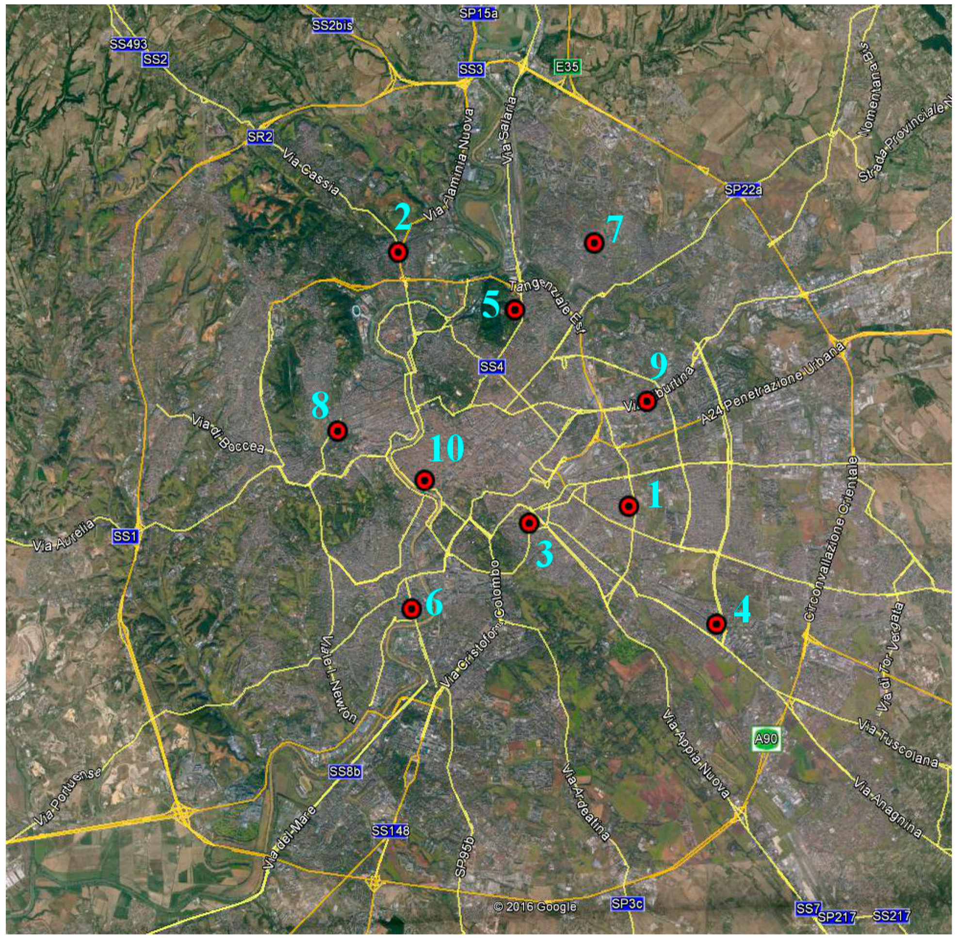
Figure 1. Google Earth map of Rome. Red circles are the monitoring stations taken into account.
Sustainability 08 00838 g001
Figure 2. Mean (blue) and standard deviation (red) values calculated for all pollutant species in the different stations. Blue line is the mean of the mean values of the different stations and the red line is the mean of the standard deviation values of the different stations. (a) [CO]; (b) [NO]; (c) [NO2]; (d) [C6H6]; (e) [O3]; (f) [SO2]; (g) [PM2.5]; (h) [PM10].
Sustainability 08 00838 g002
Figure 3. Kurtosis (blue) and Skewness (red) values calculated for all pollutant species in the different stations. Blue line is the mean of the Kurtosis values of the different stations and the red line is the mean of the Skewness values of the different stations. (a) [CO]; (b) [NO]; (c) [NO2]; (d) [C6H6]; (e) [O3]; (f) [SO2]; (g) [PM2.5]; (h) [PM10].
Sustainability 08 00838 g003
Figure 4. Hourly annual concentration variation of C6H6 during 2015 in µg/m3.
Sustainability 08 00838 g004
Figure 5. Hourly annual concentration variation of CO during 2015 in mg/m3.
Sustainability 08 00838 g005
Figure 6. Hourly annual concentration variation of NO during 2015 in µg/m3.
Sustainability 08 00838 g006
Figure 7. Hourly annual concentration variation of NO2 during 2015 in µg/m3.
Sustainability 08 00838 g007
Figure 8. Hourly annual concentration variation of O3 during 2015 in µg/m3.
Sustainability 08 00838 g008
Figure 9. Hourly annual concentration variation of SO2 during 2015 in µg/m3.
Sustainability 08 00838 g009
Figure 10. Hourly annual concentration variation of PM2.5 during 2015 in µg/m3.
Sustainability 08 00838 g010
Figure 11. Hourly annual concentration variation of PM10 during 2015 in µg/m3.
Sustainability 08 00838 g011
Figure 12. Probability density function (red triangles) and Generalized Extreme Value fitting (blue circles) of pollutant concentrations calculated for samples acquired in a year.
Sustainability 08 00838 g012
Figure 13. Dimensionless Return level trend for all the pollutant concentrations.
Sustainability 08 00838 g013
Figure 14. Cross-correlation between pollutant concentrations; benzene concentration is taken into account as a reference signal; the time axis is normalized respect to a reference time: t* = 86,400 s.
Sustainability 08 00838 g014
Figure 15. Poincaré sections [C6H6] over [NO] (a) and [C6H6] over [O3] (b).
Sustainability 08 00838 g015
Table 1. Directive 2008/50/EC standards of main pollutant.
PollutantConcentrationAveraging PeriodPermitted Excess Each Year
PM1050 µg/m324 h35
PM1040 µg/m31 year-
PM2.525 µg/m31 year-
NO2200 µg/m31 h18
NO240 µg/m31 year-
SO2350 µg/m31 h24
SO2125 µg/m324 h3
O3120 µg/m3Maximum daily 8 h mean25 days averaged over 3 years
CO10 mg/m3Maximum daily 8 h mean-
C6H65 µg/m31 year-
Table 2. Sensors used for each concentration measurement.
PollutantPMsNOxSO2O3COC6H6
SensorsMP101MCM200 A-APITE 43iM400E APITE 48iAIR Toxic
SWAMDC FAI
SWAM5a FAI
M100E APIM300E APICP 7001
SWAM DC FAI
TE SHARP 5030
Table 3. Kurtosis and Skewness values calculated for all pollutant species.
SpecieKurtosisSkewnessCoefficient of Variation
[CO]14.32.766%
[NO]17.13.3155%
[SO2]9.62.291%
[C6H6]9.42.172%
[NO2]3.90.748%
[PM2.5]4.21.360%
[PM10]3.71.046%
[O3]2.80.780%