
The Development and Full-Scale Experimental Validation of an Optimal Water Treatment Solution in Improving Chiller Performances

Abstract
:1. Introduction
- -
- Qe is the cooling capacity of a chiller on the evaporator side, kW;
- -
- P is the power consumption of a chiller compressor, kW; and
- -
- Qc is the heat dissipation on the chiller condenser side through cooling towers, kW.
- -
- Ta is the approach temperature of a chiller on the condenser side, °C;
- -
- Tc is the refrigerant condensing temperature of a chiller, °C; and
- -
- T2 is the cooling water temperature leaving the chiller condenser to the cooling tower, or simply, cooling water leaving temperature, °C.
2. A Comparative Analysis on Existing Methods to Keep Ta Smaller
- (1)
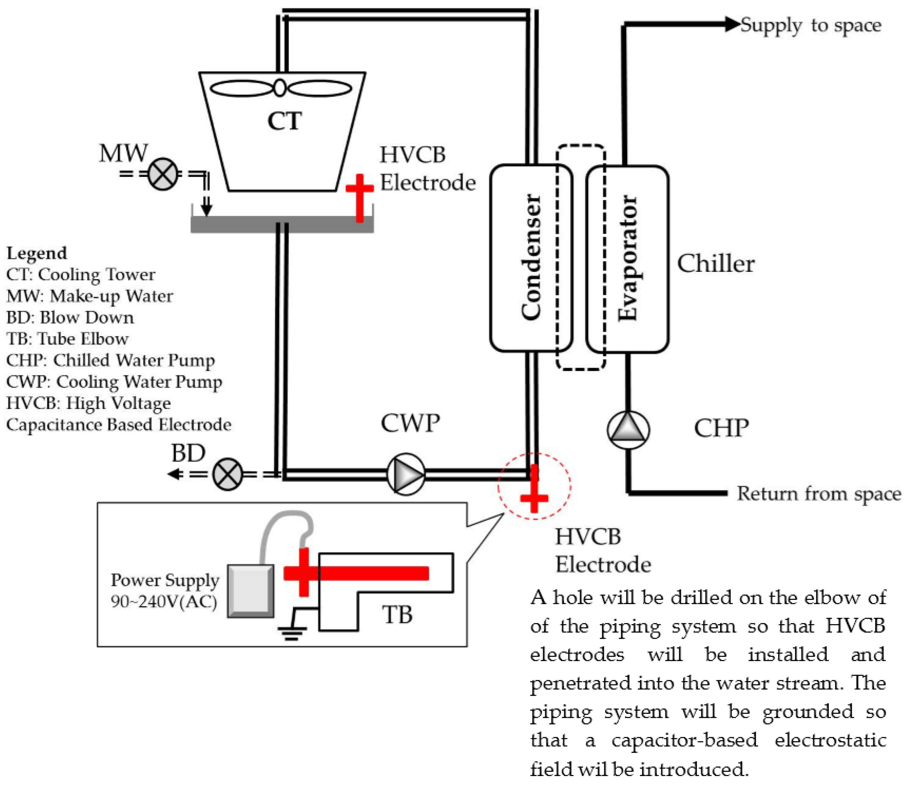
- An optimal solution, in combining physical with chemical treatment, will be developed. A high tension electrodes system, namely HVCB electrodes, also used by Romo and Pitts, coupled with biocides will be experimented.
- (2)
- Industrial full-scale tests, instead of laboratory tests, will be conducted. Chiller plants at the size of 5000 RT to 10,000 RT cooling capacities will be selected as the test sites for experiment.
- (3)
- Tests will be conducted and recorded on an annual basis, to identify the sustainability of this solution for commercial operations.
3. Theoretical Analysis on Chiller Performances
4. Experimental Investigation
4.1. Experimental Procedure
- Step 1:
- Perform all chiller COP measurement before the treatment, as a baseline for comparison.
- Step 2:
- Select an experimental chiller, divert the cooling load to a spare chiller, close the gate valve and drain its cooling water loop.
- Step 3:
- Drill a hole and weld the adaptor on the chiller condenser cooling water entry pipe, preferably at the elbow, then install the electrodes on site. It will take around 4 to 8 h to complete one rod installation.
- Step 4:
- Set up the power supply and test it, and identify that it could introduce around 30 kV to 35 kV continuous DC voltage at the site. As the electrode is not in direct contact with water, only a capacitor-based electrostatic field is introduced.
- Step 5:
- Reverse step 2 and put the experimental chiller back on duty. Rotate in the same order, until all experimental chillers are installed with electrodes system.
- Step 6:
- Switch on the power supply and begin all data-recording automatically.
- Step 7:
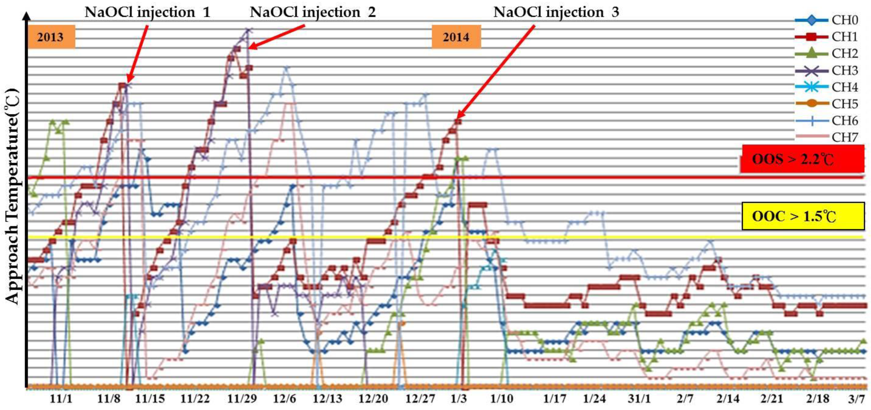
- Observe until the Ta begin to rise, which indicates that the first phase of scale and biofilm from the cooling tower fins is falling, causing the cooling water loop to be even dirtier than before. When the Ta reaches over 3 °C, input the biocide into the cooling tower, with 25 kg to 30 kg sodium hypochlorite (NaOCl). Close the blowdown valve, or raise its conductivity settings, of the cooling tower and keep it overnight.
- Step 8:
- Expect the Ta to drop significantly following the biocide input, to lower than 1 °C level on the following day. Drain the cooling tower and clean the basin.
- Step 9:
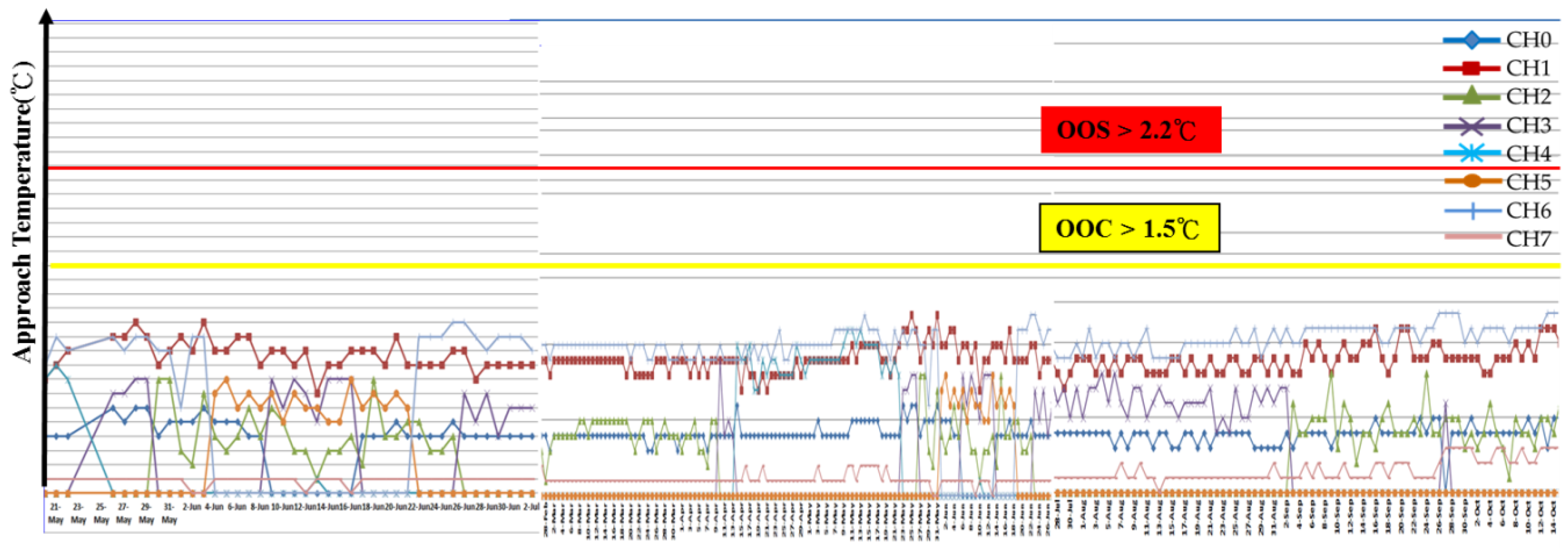
- Repeat Steps 7 and 8 until the Ta no longer shoots up over the 2.2 °C level, indicating the whole cooling water loop is clean.
- Step 10:
- Perform post-treatment chillers COP measurement to verify the energy-saving effectiveness and keep tracking it.
- Step 11:
- Allow the chiller plant to run under its normal commercial operation until the completion of the experimental investigation, preferably for over one or two years. Keep track on its Ta variation during the whole period of time from the automatic data acquisition system.
4.2. Measurement and Verification Methodology on the COP Improvement
- (1)
- The circumference of one of the cooling water pipes and the circumference of one of the insulated chilled water pipes shall be measured using a measuring tape. The outer diameter of the cooling water pipe shall be computed and keyed into the portable ultrasonic flow meter.
- (2)
- A rectangular portion of the insulation foam, measuring 60 cm × 12 cm shall be removed from the exterior of the chilled water pipe. On the wall of each piping system chosen from the chilled water and cooling water loop, a pair of flow rate transducers of the flow meter will be installed by choosing a location of reasonable distance, normally around six pipe diameters in distance away from piping fittings, including elbows and valves to avoid flow turbulence resulting in bad readings.
- (3)
- Besides the chilled water and cooling water flow rates, the following parameters shall be measured every three seconds for three days, including:
- (a)
- cooling water outlet temperature (T1);
- (b)
- cooling water inlet temperature (T2);
- (c)
- chilled water inlet temperature (T3);
- (d)
- chilled water outlet temperature (T4);
- (e)
- condenser output (Qc), as shown in Equation (2); and
- (f)
- evaporator output (Qe), as shown in Equation (2).
- (4)
- The length of measurement time shall be extended until the following criteria are met:
- (a)
- fluctuation of water flow rates to be within the range of ±5%;
- (b)
- fluctuation of all inlet and outlet temperatures to be within the range of ±0.5 °C; and
- (c)
- compliance with Equation (2) to stay within 5% engineering tolerances.
- (5)
- After 60 days, the above-mentioned procedure will be repeated for the post-treatment COP measurements.
5. Experimental Results and Discussion
5.1. UH Plant Chiller Data
5.2. GF Plant Data
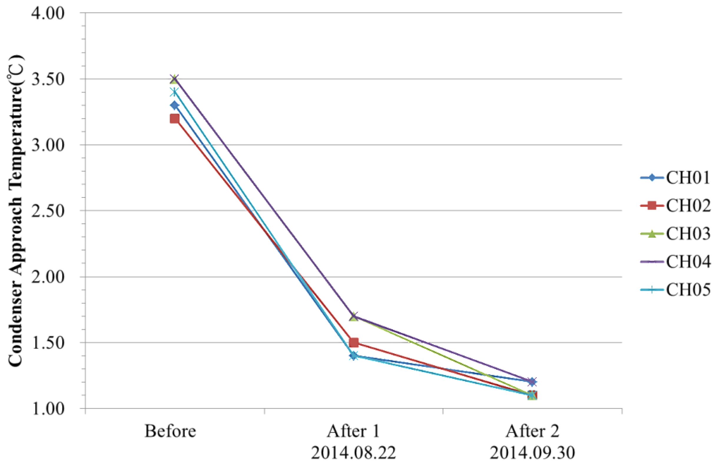
The Ta Data Analysis
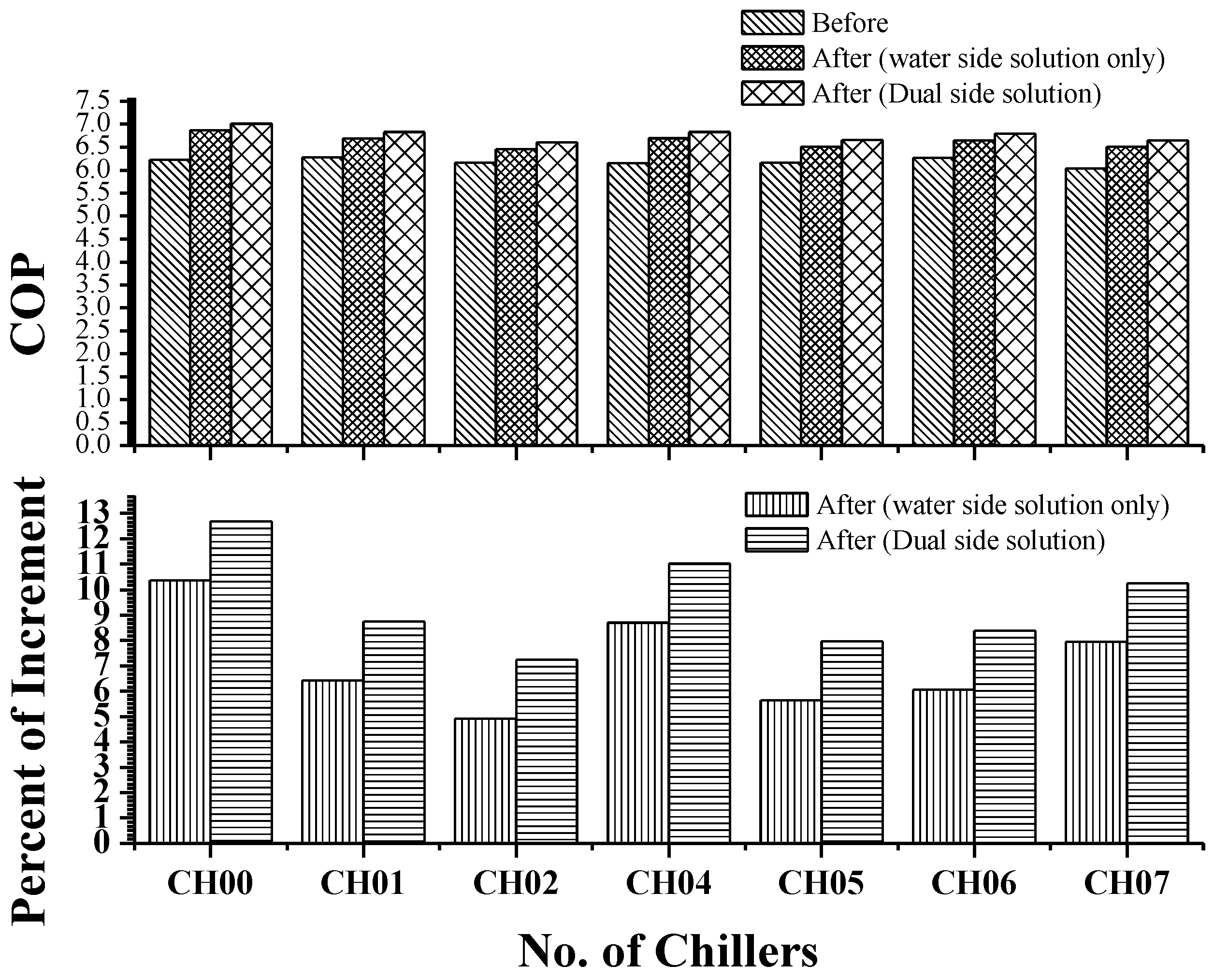
- (1)
- The Energy-Savings Effect of the GF Plant
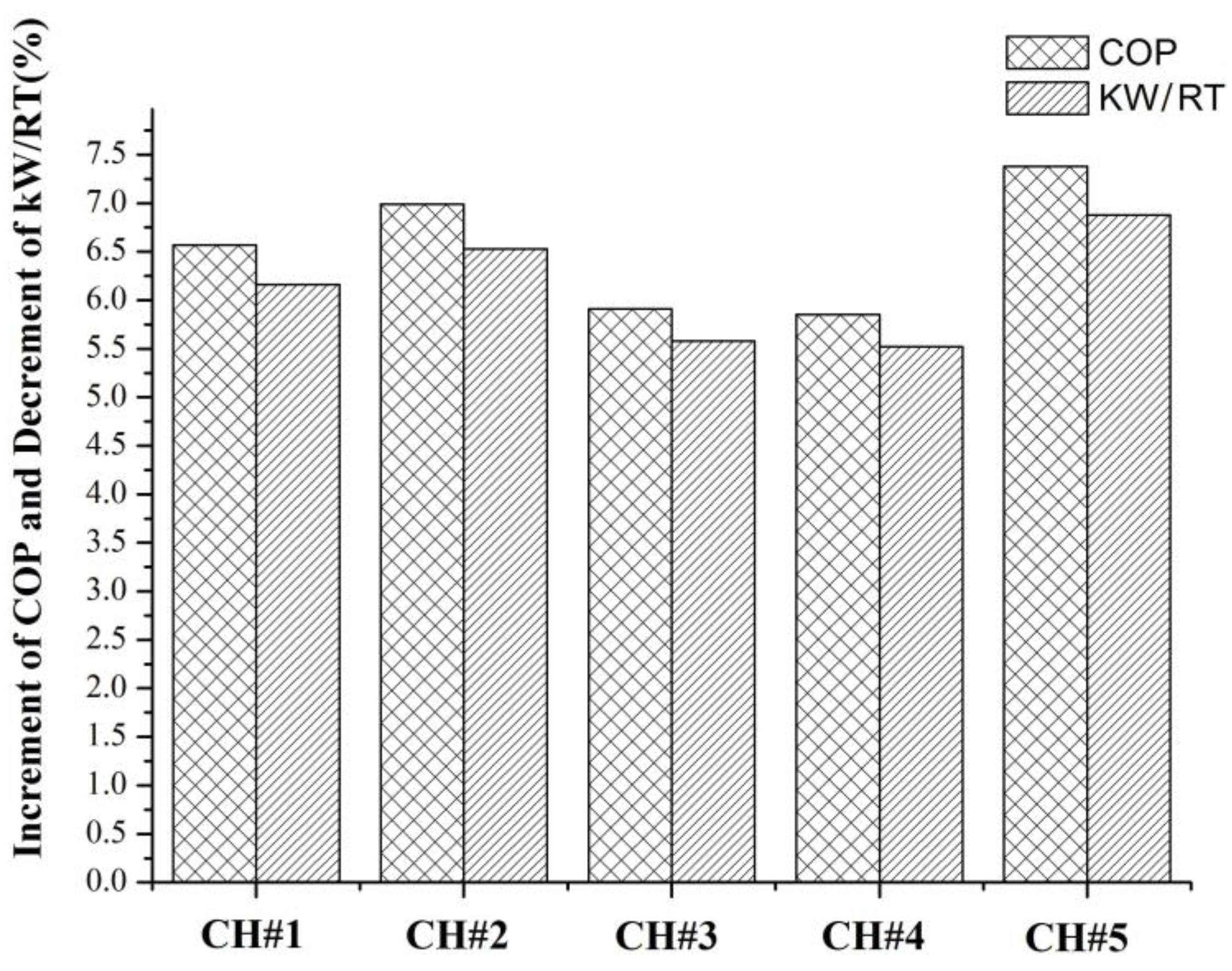
- (2)
- To Identify the Energy Savings Contribution by the Electrodes Alone
5.3. Cooling Tower System for Scaling Mitigation and Chemical Reduction
5.3.1. The Chemical Reduction Issue
- (1)
- To record the accumulated fallen deposit amount on the cooling tower basin and the side filter screen after the 35 kV DC electrodes’ implementation.
- (2)
- To perform a systematic chemical dosage reduction phase, sampling the water for quality analysis in due course. Optimize between the chemical dosage and the acceptable water quality.
- (3)
- To Record the blowdown and make-up water quantity during treatment and identify the water conservation effectiveness.
5.3.2. Results and Discussions for Step 1
5.3.3. Results and Discussions for Step 2
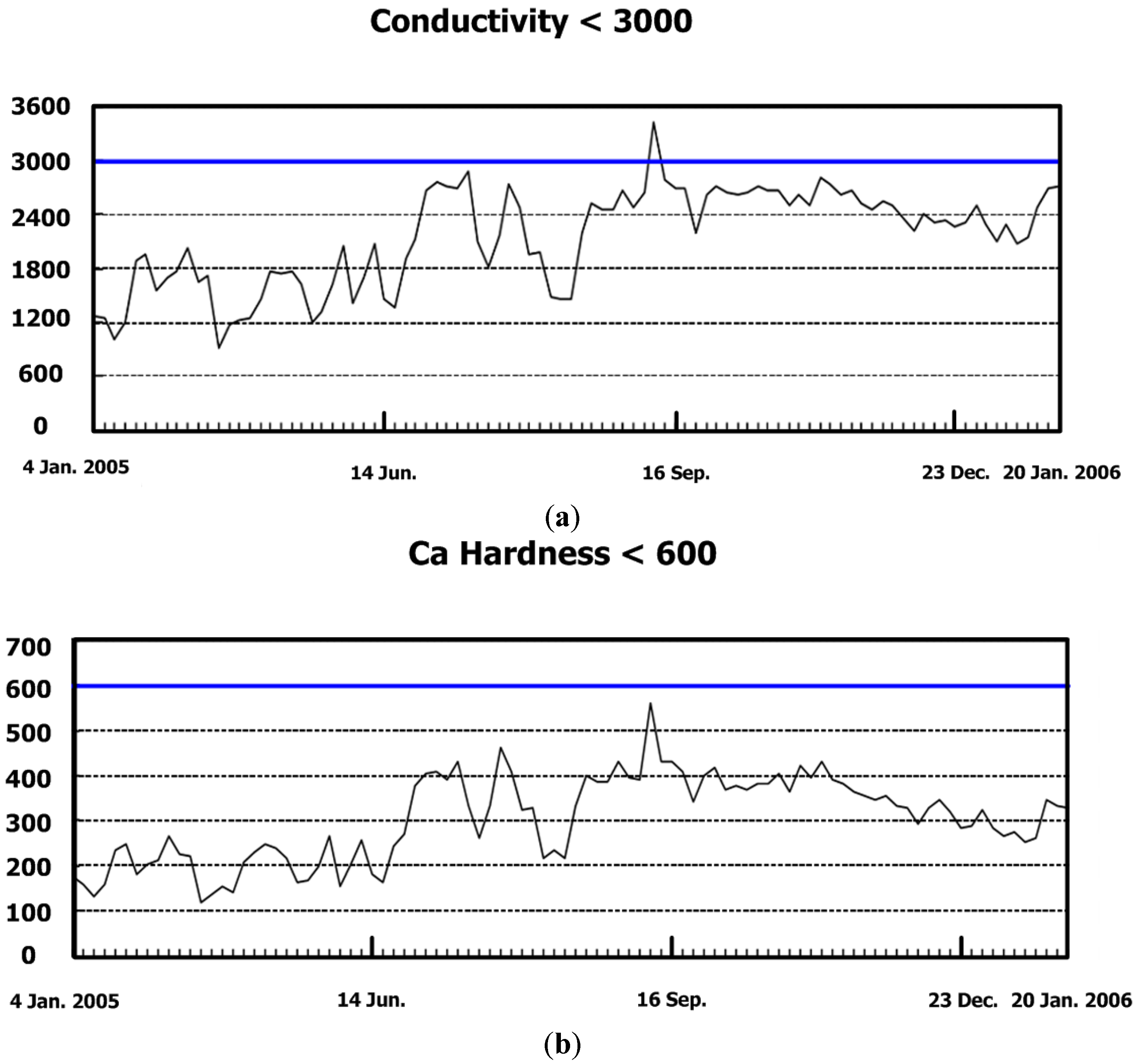
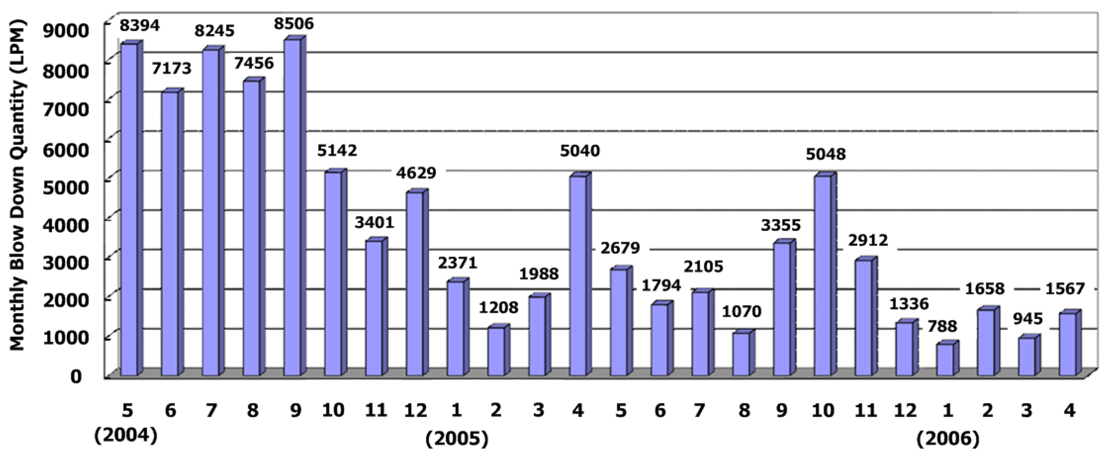
5.3.4. Results and Discussions for Step 3
6. Conclusions and Recommendations
Acknowledgments
Author Contributions
Conflicts of Interest
Abbreviations
| COP | Coefficient of performance |
| CFCs | Chlorofluorocarbons |
| HVAC | Heating, ventilation and air conditioning |
| HVCB | High voltage capacitance based |
| CH | Chiller |
| DC | Direct current |
| M & V | Measurement and verification |
| SCADA | Supervisory control and data acquisition system |
| L | Part load factor |
| P | Power consumption of a chiller compressor |
| Q | Cooling capacity or heat dissipation on the chiller |
| T | Temperature |
| Subscripts | |
| a | approach temperature |
| c | condenser |
| e | evaporator |
| 1 | leaving condenser |
| 2 | entering condenser |
| 3 | entering evaporator |
| 4 | leaving evaporator |
References
- ASHRAE. Refrigeration Handbook; ASHRAE: Atlanta, GA, USA, 2006; Section 7.4. [Google Scholar]
- Stoecker, W.F.; Jones, J.W. Compressors. In Refrigeration and Air Conditioning, 2nd ed.; McGraw-Hill, Inc.: New York, NY, USA, 1982. [Google Scholar]
- ASHRAE. ASHRAE. In HVAC Systems and Equipment Handbook; ASHRAE: Atlanta, GA, USA, 2000; Volume 35, pp. 7–8. [Google Scholar]
- Muilenberg, T.; Candir, C. How stripping biofilm from the cooling water loop impacts power plant production output. In Proceedings of the Cooling Technology Institute Annual Conference, Corpus Christi, TX, USA, 3–7 February 2013.
- Baker, J.S.; Judd, S.J. Magnetic amelioration of scale formation. Water Res. 1996, 30, 247–260. [Google Scholar] [CrossRef]
- Barrett, R.A.; Parsons, S.A. The influence of magnetic fields on calcium carbonate precipitation. Water Res. 1998, 32, 609–612. [Google Scholar] [CrossRef]
- Kim, W.T.; Cho, Y.I.; Bai, C. Effect of electronic anti-fouling treatment on fouling mitigation with circulating cooling tower water. Int. J. Commun. Heat Mass Transf. 2001, 28, 671–680. [Google Scholar] [CrossRef]
- Xing, Z.K. Research on the electromagnetic anti-fouling technology for heat transfer enhancement. Appl. Therm. Eng. 2008, 28, 889–894. [Google Scholar]
- Cho, Y.I.; Fan, C.F.; Choi, B.G. Theory of Electronic Anti-Fouling Technology to Control Precipitation Fouling in Heat Exchangers. Int. J. Commun. Heat Mass Transf. 1997, 24, 747–756. [Google Scholar] [CrossRef]
- Cho, Y.I.; Lee, S.H. Reduction in the surface tension of water due to physical water treatment for fouling control in heat exchangers. Int. J. Commun. Heat Mass Transf. 2005, 32, 1–19. [Google Scholar] [CrossRef]
- Cho, Y.I. Efficiency of Physical Water Treatments in Controlling Calcium Scale Accumulation in Recirculating Open Cooling Water System; ASHRAE Final Report, ASHRAE Research Project; Old City Publishing, Inc.: Philadelphia, PA, USA, 2002; p. 1155-TRP. [Google Scholar]
- Cho, Y.I.; Lee, S.H.; Kim, W. Physical water treatment for the mitigation of mineral fouling in cooling-tower water applications. ASHRAE Trans. 2003, 109, 346–357. [Google Scholar]
- Romo, R.F.V.; Pilts, M.M. Application of Electrotechnology for Removal and Prevention of Reverse Osmosis. Biofouling Environ. Prog. 1999, 18, 107–112. [Google Scholar] [CrossRef]
- Cho, Y.I.; Taylor, W.T. An innovative electronic descaling technology for scale prevention in a chiller. ASHRAE Trans. Symp. 1999, 105, 581–586. [Google Scholar]
- SOLKANE Refrigerant Software Version 8.0. All Rights Reserved by Solvay Flour GmbH Hannover 2012. Available online: http://www.solvay.us/en/binaries/SOLKANE_Refrigerants-238168.pdf (accessed on 23 September 2015).


| Ta (°C) | Tc (°C) | Qe (°C) | P (kW) | COP | kW/RT | Percentage of Increase COP | Percentage of Reduction kW/RT |
|---|---|---|---|---|---|---|---|
| 3.0 | 37.2 | 3811 | 612 | 6.22 | 0.565 | 0 (Base) | 0 (Base) |
| 2.8 | 37.0 | 3842 | 612 | 6.27 | 0.561 | 0.80 | −0.80 |
| 2.6 | 36.8 | 3872 | 613 | 6.32 | 0.556 | 1.61 | −1.58 |
| 2.4 | 36.6 | 3903 | 614 | 6.36 | 0.553 | 2.25 | −2.20 |
| 2.2 | 36.4 | 3934 | 615 | 6.4 | 0.549 | 2.89 | −2.81 |
| 2.0 | 36.2 | 3965 | 615 | 6.44 | 0.546 | 3.54 | −3.42 |
| 1.8 | 36.0 | 3995 | 616 | 6.49 | 0.542 | 4.34 | −4.16 |
| 1.6 | 35.8 | 4026 | 616 | 6.53 | 0.538 | 4.98 | −4.75 |
| 1.4 | 35.6 | 4057 | 617 | 6.58 | 0.534 | 5.79 | −5.47 |
| 1.2 | 35.4 | 4088 | 617 | 6.62 | 0.531 | 6.43 | −6.04 |
| 1.0 | 35.2 | 4118 | 618 | 6.67 | 0.527 | 7.23 | −6.75 |
| 0.8 | 35.0 | 4149 | 618 | 6.71 | 0.524 | 7.88 | −7.30 |
| 0.6 | 34.8 | 4180 | 618 | 6.76 | 0.520 | 8.68 | −7.99 |
| 0.4 | 34.6 | 4210 | 619 | 6.81 | 0.516 | 9.49 | −8.66 |
| 0.2 | 34.4 | 4241 | 619 | 6.85 | 0.513 | 10.13 | −9.20 |
| 0.0 | 34.2 | 4272 | 619 | 6.9 | 0.510 | 10.93 | −9.86 |
| Cooling Water Flow | Chilled Water Flow | Power | COP | |||||||
|---|---|---|---|---|---|---|---|---|---|---|
| Outlet, T1 | Inlet, T2 | Flow Rate | QC | Inlet, T3 | Outlet, T4 | Flow Rate | Qe | P | ||
| (°C) | (°C) | (LPM) | (kW) | (°C) | (°C) | (LPM) | (kW) | (kW) | (kW/kW) | |
| 1 | 33.50 | 29.20 | 16,302.07 | 4890.62 | 18.00 | 13.40 | 13,012.11 | 4175.98 | 609.42 | 6.85 |
| 2 | 33.50 | 29.20 | 16,325.57 | 4897.67 | 18.00 | 13.50 | 13,555.80 | 4255.89 | 609.48 | 6.98 |
| 3 | 33.50 | 29.20 | 16,307.10 | 4892.13 | 18.10 | 13.50 | 13,011.36 | 4175.74 | 608.97 | 6.86 |
| 4 | 33.50 | 29.20 | 16,430.13 | 4929.04 | 18.10 | 13.50 | 13,051.68 | 4188.68 | 609.47 | 6.87 |
| 5 | 33.50 | 29.20 | 16,396.67 | 4919.00 | 18.10 | 13.50 | 13,096.96 | 4203.21 | 609.42 | 6.90 |
| 6 | 33.50 | 29.30 | 16,687.79 | 4889.91 | 18.10 | 13.50 | 13,211.78 | 4240.06 | 609.39 | 6.96 |
| 7 | 33.60 | 29.40 | 16,581.72 | 4858.83 | 18.10 | 13.50 | 13,135.57 | 4215.60 | 610.28 | 6.91 |
| 8 | 33.60 | 29.40 | 16,721.03 | 4899.65 | 18.10 | 13.60 | 13,515.12 | 4243.12 | 610.64 | 6.95 |
| 9 | 33.70 | 29.50 | 16,643.15 | 4876.83 | 18.20 | 13.60 | 13,067.73 | 4193.83 | 611.03 | 6.86 |
| 10 | 33.80 | 29.60 | 16,607.56 | 4866.40 | 18.20 | 13.60 | 13,052.15 | 4188.83 | 611.82 | 6.85 |
| 11 | 33.80 | 29.60 | 16,549.37 | 4849.35 | 18.20 | 13.60 | 13,074.49 | 4196.00 | 612.26 | 6.85 |
| 12 | 33.90 | 29.70 | 16,599.74 | 4864.11 | 18.20 | 13.70 | 13,404.31 | 4208.33 | 612.50 | 6.87 |
| 13 | 33.90 | 29.70 | 16,512.75 | 4838.62 | 18.30 | 13.70 | 13,133.01 | 4214.78 | 613.20 | 6.87 |
| 14 | 34.00 | 29.80 | 16,726.97 | 4901.39 | 18.30 | 13.70 | 13,043.96 | 4186.20 | 613.63 | 6.82 |
| 15 | 34.00 | 29.80 | 16,758.50 | 4910.63 | 18.30 | 13.70 | 13,157.07 | 4222.50 | 614.95 | 6.87 |
| 16 | 34.10 | 29.80 | 16,380.33 | 4914.10 | 18.30 | 13.70 | 13,187.04 | 4232.12 | 617.45 | 6.85 |
| 17 | 34.10 | 29.90 | 16,704.13 | 4894.70 | 18.30 | 13.70 | 13,078.86 | 4197.40 | 618.50 | 6.79 |
| 18 | 34.20 | 29.90 | 16,501.20 | 4950.36 | 18.30 | 13.70 | 13,156.35 | 4222.27 | 620.16 | 6.81 |
| 19 | 34.20 | 30.00 | 16,889.44 | 4949.00 | 18.30 | 13.70 | 13,267.21 | 4257.85 | 622.92 | 6.84 |
| 20 | 34.30 | 30.00 | 16,583.30 | 4974.99 | 18.30 | 13.70 | 13,261.79 | 4256.11 | 625.56 | 6.80 |
| 21 | 34.30 | 30.00 | 16,713.33 | 5014.00 | 18.40 | 13.70 | 13,107.31 | 4297.98 | 628.38 | 6.84 |
| 22 | 34.40 | 30.10 | 16,797.37 | 5039.21 | 18.40 | 13.70 | 13,028.57 | 4272.16 | 631.83 | 6.76 |
| 23 | 34.40 | 30.10 | 16,711.17 | 5013.21 | 18.40 | 13.70 | 13,032.45 | 4273.43 | 632.99 | 6.75 |
| 24 | 34.50 | 30.10 | 16,507.63 | 5067.46 | 18.40 | 13.70 | 13,226.56 | 4337.08 | 635.42 | 6.83 |
| 25 | 34.50 | 30.10 | 16,491.67 | 5062.56 | 18.40 | 13.70 | 13,267.09 | 4350.37 | 637.77 | 6.82 |
| 26 | 34.40 | 30.10 | 17,016.87 | 5105.06 | 18.50 | 13.70 | 12,967.55 | 4342.62 | 638.15 | 6.81 |
| 27 | 34.40 | 30.00 | 16,636.93 | 5107.15 | 18.40 | 13.70 | 13,189.01 | 4324.77 | 639.52 | 6.76 |
| 28 | 34.40 | 30.00 | 16,668.01 | 5116.69 | 18.40 | 13.70 | 13,328.14 | 4370.39 | 641.31 | 6.81 |
| 29 | 34.40 | 30.00 | 16,638.20 | 5107.54 | 18.40 | 13.70 | 13,300.78 | 4361.42 | 640.99 | 6.80 |
| 30 | 34.40 | 30.00 | 17,055.88 | 5235.76 | 18.40 | 13.60 | 13,002.60 | 4354.36 | 640.54 | 6.80 |
| 31 | 34.30 | 29.90 | 17,103.77 | 5250.46 | 18.40 | 13.60 | 12,987.10 | 4349.17 | 640.64 | 6.79 |
| 32 | 34.10 | 29.80 | 17,277.43 | 5183.23 | 18.30 | 13.60 | 13,202.37 | 4329.15 | 640.98 | 6.75 |
| 33 | 33.90 | 29.60 | 17,423.53 | 5227.06 | 18.30 | 13.50 | 13,023.18 | 4361.25 | 637.16 | 6.84 |
| 34 | 33.70 | 29.30 | 17,080.58 | 5243.34 | 18.30 | 13.50 | 13,070.90 | 4377.23 | 633.85 | 6.91 |
| 35 | 33.50 | 29.20 | 17,461.40 | 5238.42 | 18.20 | 13.50 | 13,259.71 | 4347.95 | 633.23 | 6.87 |
| 36 | 33.40 | 29.10 | 17,315.90 | 5194.77 | 18.20 | 13.40 | 12,976.86 | 4345.74 | 630.75 | 6.89 |
| 37 | 33.30 | 29.10 | 17,541.10 | 5139.95 | 18.10 | 13.40 | 13,305.05 | 4362.82 | 629.24 | 6.93 |
| 38 | 33.30 | 29.00 | 16,943.40 | 5083.02 | 18.10 | 13.40 | 13,195.39 | 4326.86 | 626.78 | 6.90 |
| 39 | 33.20 | 29.00 | 17,385.04 | 5094.22 | 18.10 | 13.40 | 13,122.81 | 4303.06 | 621.63 | 6.92 |
| 40 | 33.20 | 28.90 | 16,882.37 | 5064.71 | 18.10 | 13.40 | 13,088.62 | 4291.85 | 621.09 | 6.91 |
| 41 | 33.10 | 28.90 | 17,194.06 | 5038.26 | 18.00 | 13.40 | 13,493.24 | 4330.39 | 616.35 | 7.03 |
| 42 | 33.00 | 28.90 | 17,392.03 | 4974.93 | 18.10 | 13.40 | 13,157.27 | 4314.36 | 613.70 | 7.03 |
| 43 | 33.10 | 28.90 | 16,931.08 | 4961.20 | 18.10 | 13.40 | 13,039.64 | 4275.79 | 612.39 | 6.98 |
| 44 | 33.10 | 28.90 | 16,947.70 | 4966.07 | 18.00 | 13.40 | 13,350.07 | 4284.44 | 612.07 | 7.00 |
| Chiller CH00 | ||
|---|---|---|
| Pre-Treatment 9 September 2013 2:07 p.m. | Post Treatment 25 October 2013 1:38 p.m. | |
| Loading % | 89 | 89 |
| Power Consumption (kW) | 612.58 | 618.89 |
| Refrigerant Capacity, Qe | 3810.55 | 4271.50 |
| COP | 6.22 | 6.90 |
| kW/RT | 0.565 | 0.509 |
| Change in COP (Improved) | 10.95% | |
| Change in kW/RT (Reduced) | −9.87% | |
| Name of Item | Before | After |
|---|---|---|
| Date | 4 July 2013 | 1 September 2013 |
| Time | 07:48:42 a.m. | 01:17:52 a.m. |
| Cooling Water Flow Rate (LPM) | 3193.06 | 3196.19 |
| T1 (°C) | 33.7 | 33.6 |
| T2 (°C) | 28.5 | 28.5 |
| Qc (kW) | 533.52 | 533.56 |
| Chilled Water Flow Rate (LPM) | 2586.83 | 2590.16 |
| T3 (°C) | 12.7 | 12.7 |
| T4 (°C) | 6.2 | 6.2 |
| Loading (%) | 59% | 59% |
| Qe (kW) | 339.89 | 339.34 |
| Power Consumption | 508.7 | 497.8 |
| COP | 5.09 | 5.20 |
| kW/RT | 0.69 | 0.68 |
| Improvement of COP | 2.32% | |
| Reduction of kW/RT | 2.26% | |
| Total Weight of Colloids Collected | Utility Plant A | EG Plant B | ||
|---|---|---|---|---|
| 24,000 RT | 20,000 RT | |||
| With Electrodes | Without Electrodes | |||
| Cleaning Time | Weight Collected at the Cooling Tower Basin, kg Per Month | No. of Weeks | Weight Collected at the Filter, kg/week | Weight Collected at the Filter, kg/week |
| 1st month | Negligible, in either plant A or plant B | 1 | 0.5 | 0 |
| 2 | 2.3 | 0 | ||
| 3 | 0.6 | 0 | ||
| 4 | 1.3 | 0 | ||
| 2nd month | 500 kg at Plant A | 5 | 1.8 | 0 |
| 6 | 2.0 | 0 | ||
| 7 | 1.2 | 0 | ||
| 8 | 1.4 | 0 | ||
| 3rd month | 550 kg at Plant A | 9 | 1.2 | 0 |
| 10 | 2.0 | 0 | ||
| Average | 1.43 kg per week | negligible | ||
| Sample | 1 | 2 | ||||
|---|---|---|---|---|---|---|
| Test Data | 4 March 2002 | 2 May 2002 | ||||
| Composition | Plant A Cooling Towers (With Electrodes) | Plant B Cooling Towers (Without Electrodes) | Plant A Cooling Towers (With Electrodes) | Plant B Cooling Towers (Without Electrodes) | BAP Plant Cooling Tower (Without Electrodes) | EPOXY Plant Cooling Tower (Without Electrodes) |
| S (SO3) | 0.856 | 1.712 | 0.579 | 1.423 | 0.661 | 0.578 |
| Fe (Fe2O3) | 1.391 | 1.59 | 0.18 | 1.32 | 2.662 | 2.026 |
| Ni | <0.003 | >0.009 | 0.003 | 0.009 | 0.019 | 0.007 |
| Al (Al2O3) | 1.893 | 2.984 | 0.231 | 1.961 | 1.262 | 2.869 |
| Ca (CaCO3) ▲ | 19.324 | 2.492 | 17.572 | 2.071 | 1.391 | 8.201 |
| Si (SiO2) | 12.051 | 18.951 | 11.2 | 16.094 | 5.704 | 15.928 |
| Cu (CuO) | 0.038 | 0.097 | 0.019 | 0.014 | 0.042 | 0.01 |
| Cl | 0.077 | 0.11 | 0.082 | 0.138 | 0.143 | 0.144 |
| Na (Na2O) | 0.465 | 0.143 | 0.383 | >0.143 | 0.663 | 0.44 |
| Ba | <0.001 | >0.001 | <0.001 | 0.091 | 0.053 | 0.18 |
| Mg (MgO) | 0.813 | 1.055 | 1.047 | 3.095 | 0.241 | 2.886 |
| Y (Y2O3) | >0.001 | >0.001 | <0.001 | 0.001 | >0.001 | 0.002 |
| Cr (Cr2O3) | 0.012 | 0.277 | 0.004 | 0.017 | 0.039 | 0.046 |
| Mn (MnO) | 0.035 | 0.053 | 0.026 | 0.03 | >0.030 | 0.035 |
| Br | 0.016 | 0.143 | 0.014 | 0.054 | 0.008 | 0.002 |
| K (K2O) | 0.352 | 0.43 | 0.169 | 0.667 | 0.682 | 1.045 |
| Zr (ZrO2) | 0.008 | 0.009 | <0.007 | 0.012 | 0.007 | 0.021 |
| Rb | <0.003 | >0.003 | <0.003 | >0.003 | 0.003 | 0.006 |
| P (P2O5) | 0.125 | 0.715 | 0.051 | 0.235 | 0.986 | 1.919 |
| Zn (ZnO) | 0.357 | 6.494 | <1.800 | 3.112 | 1.814 | 0.114 |
| Ti (TiO2) | 0.164 | 0.257 | 0.031 | 0.015 | 0.013 | 0.038 |
| As (As2O3) | 0.009 | 0.228 | 0.006 | 0.023 | 0.024 | 0.004 |
| pH Value | Conductivity μs/cm | Ca Hardness ppm | Suspended Solid ppm | Turbidity NTU |
|---|---|---|---|---|
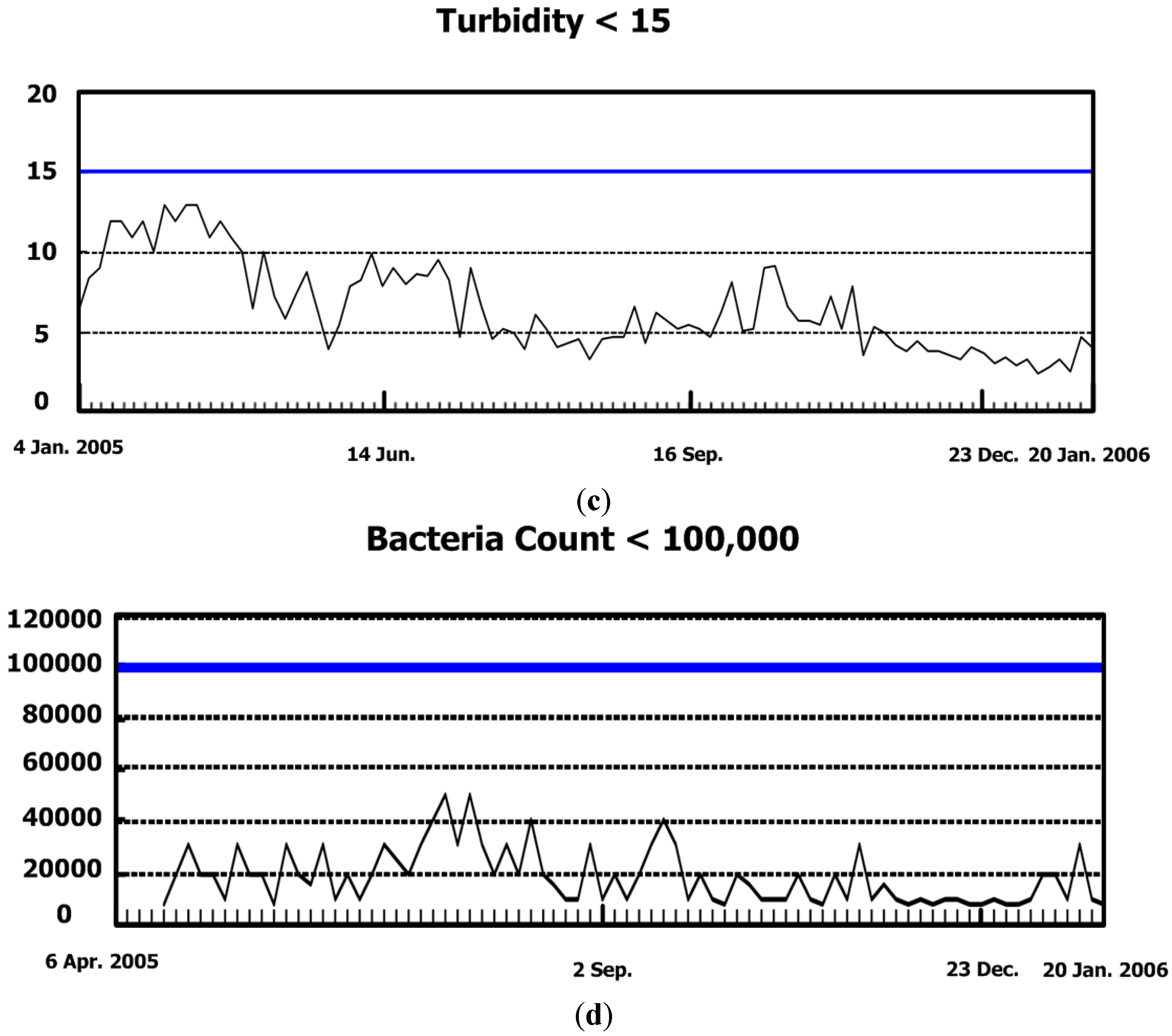
| 7–9 | <2500 | <450 | <10 | <15 |
| Free Cl ppm | Bacteria Count CFU/100 mL | Cycles of Concentration | Corrosion rate mpy (Fe) | |
| 0.1–0.2 | <100,000 | <5 | <2 |
| Chemicals Added | Existing Dosage | Adjustment Stages | ||||||||
|---|---|---|---|---|---|---|---|---|---|---|
| 1 | 2 | 3 | 4 | |||||||
| 1 Apr. to 31 May | 1 Jun. to 30 Jun. | 1 Jul. to 31 Jul. | 1 Aug. to 31 Aug. | 1 Sept. to 30 Sept. | 1 Oct. to 31 Oct. | 1 Nov. to 30 Nov. (Originally Planned) | 9 Nov. (Actually Executed) | 23 Dec. | ||
| Sulfuric acid | 100% | 100% | 100% | 100% | 100% | 100% | 100% | 100% | 75% | 0% |
| Sodium Hypochlorite | 100% | 75% | 75% | 75% | 75% | 75% | 75% | 75% | 75% | 75% |
| Biocide | 100% | 75% | 75% | 75% | 75% | 50% | 25% | 0% | 0% | 0% |
| Corrosion inhibitor | 100% | 75% | 50% | 25% | 0% | 0% | 0% | 0% | 25% | 25% |
| Year | Date | pH Value | Conductivity μs/cm | Ca Hardness ppm | Suspended Solid ppm | Turbidity NTU | Free Cl ppm | Bacteria Count CFU/100 mL | Cycles | Weekly Water Discharge Rate LPM | Corrosion Rate mpy (Fe) | |
|---|---|---|---|---|---|---|---|---|---|---|---|---|
| 7–9 | <3000 | <600 | <10 | <15 | 0.1–0.2 | <100,000 | <6 | <2 | ||||
| 2005 | 21 Apr. | 8.2 | 1222 | 155 | 7.0 | 11 | 0.10 | 8000 | 2.5 | NA | 0.64 | |
| 3 May | 8.4 | 1471 | 208 | 4.6 | 6.5 | 0.10 | 8000 | 2.9 | 0.72 | |||
| 17 May | 8.3 | 1622 | 218 | 4.2 | 7.4 | 0.05 | 20,000 | 3.8 | ||||
| 21 Jun. | 8.5 | 1921 | 244 | 5.2 | 8.0 | 0.10 | 10,000 | 3.8 | 26 | 1.02 | ||
| 1 Jul. | 8.3 | 2760 | 403 | 4.8 | 9.6 | 0.10 | 20,000 | 6.2 | 797 | 1.40 | ||
| 5 Aug. | 8.2 | 1982 | 327 | 2.6 | 5.2 | 0.10 | 20,000 | 4.4 | NA | 3.28 | ||
| 2 Sept. | 8.3 | 2480 | 394 | 3.3 | 4.3 | 0.10 | 10,000 | 5.7 | 432 | 3.71 | ||
| 7 Oct. | 8.3 | 2620 | 377 | 3.8 | 5.3 | 0.10 | 8000 | 5.2 | 692 | 4.04 | ||
| 4 Nov. | 8.3 | 2800 | 431 | 3.8 | 5.2 | 0.10 | 8000 | 6.7 | 515 | 2.78 | ||
| 2 Dec. | 8.4 | 2370 | 329 | 2.6 | 3.8 | 0.15 | 10,000 | 4.8 | 44 | 1.50 | ||
| 2006 | 17 Jan. | 8.5 | 2480 | 345 | 1.8 | 2.6 | 0.05 | 30,000 | 5.2 | NA | 1.10 | |
| 21 Feb. | 8.6 | 2630 | 319 | 1.2 | 3.1 | 0.05 | 10,000 | 4.6 | 243 | 0. 81 | ||
| 24 Mar. | 8.4 | 2980 | 413 | 1.8 | 2.6 | 0.05 | 10,000 | 5.9 | 295 | 1.20 | ||
| 21 Apr. | 8.7 | 2890 | 340 | 3.6 | 6.8 | 0.10 | 30,000 | 5.4 | 433 | 2.01 | ||
| 5 May | 8.6 | 2810 | 368 | 1.3 | 3.7 | 0.10 | 20,000 | 5.7 | 135 | 2.39 | ||
| 20 Jun. | 8.8 | 2920 | 431 | 4.2 | 6.3 | 0.10 | 10,000 | 5.2 | 387 | 2.69 | ||
| 18 Jul. | 8.7 | 2760 | 435 | 1.3 | 3.5 | 0.05 | 10,000 | 5.3 | NA | 1.83 | ||
| 22 Aug. | 8.7 | 3050 | 489 | 1.3 | 4.5 | 0.05 | 20,000 | 5.9 | 821 | 1.06 | ||
© 2016 by the authors; licensee MDPI, Basel, Switzerland. This article is an open access article distributed under the terms and conditions of the Creative Commons Attribution (CC-BY) license (http://creativecommons.org/licenses/by/4.0/).
Share and Cite
Chiang, C.-Y.; Yang, R.; Yang, K.-H. The Development and Full-Scale Experimental Validation of an Optimal Water Treatment Solution in Improving Chiller Performances. Sustainability 2016, 8, 615. https://doi.org/10.3390/su8070615
Chiang C-Y, Yang R, Yang K-H. The Development and Full-Scale Experimental Validation of an Optimal Water Treatment Solution in Improving Chiller Performances. Sustainability. 2016; 8(7):615. https://doi.org/10.3390/su8070615
Chicago/Turabian StyleChiang, Chen-Yu, Ru Yang, and Kuan-Hsiung Yang. 2016. "The Development and Full-Scale Experimental Validation of an Optimal Water Treatment Solution in Improving Chiller Performances" Sustainability 8, no. 7: 615. https://doi.org/10.3390/su8070615
APA StyleChiang, C.-Y., Yang, R., & Yang, K.-H. (2016). The Development and Full-Scale Experimental Validation of an Optimal Water Treatment Solution in Improving Chiller Performances. Sustainability, 8(7), 615. https://doi.org/10.3390/su8070615