
Modeling and Multi-Objective Optimization of NOx Conversion Efficiency and NH3 Slip for a Diesel Engine

Abstract
:1. Introduction
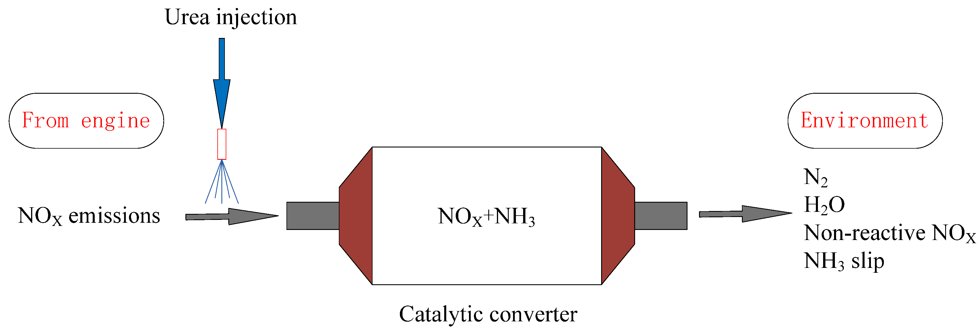
2. Experimental Setup and Methods
2.1. Data Collection
2.2. Data Preprocessing
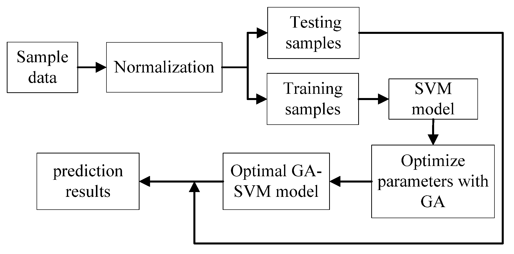
2.3. Building and Optimizing the SVM Models
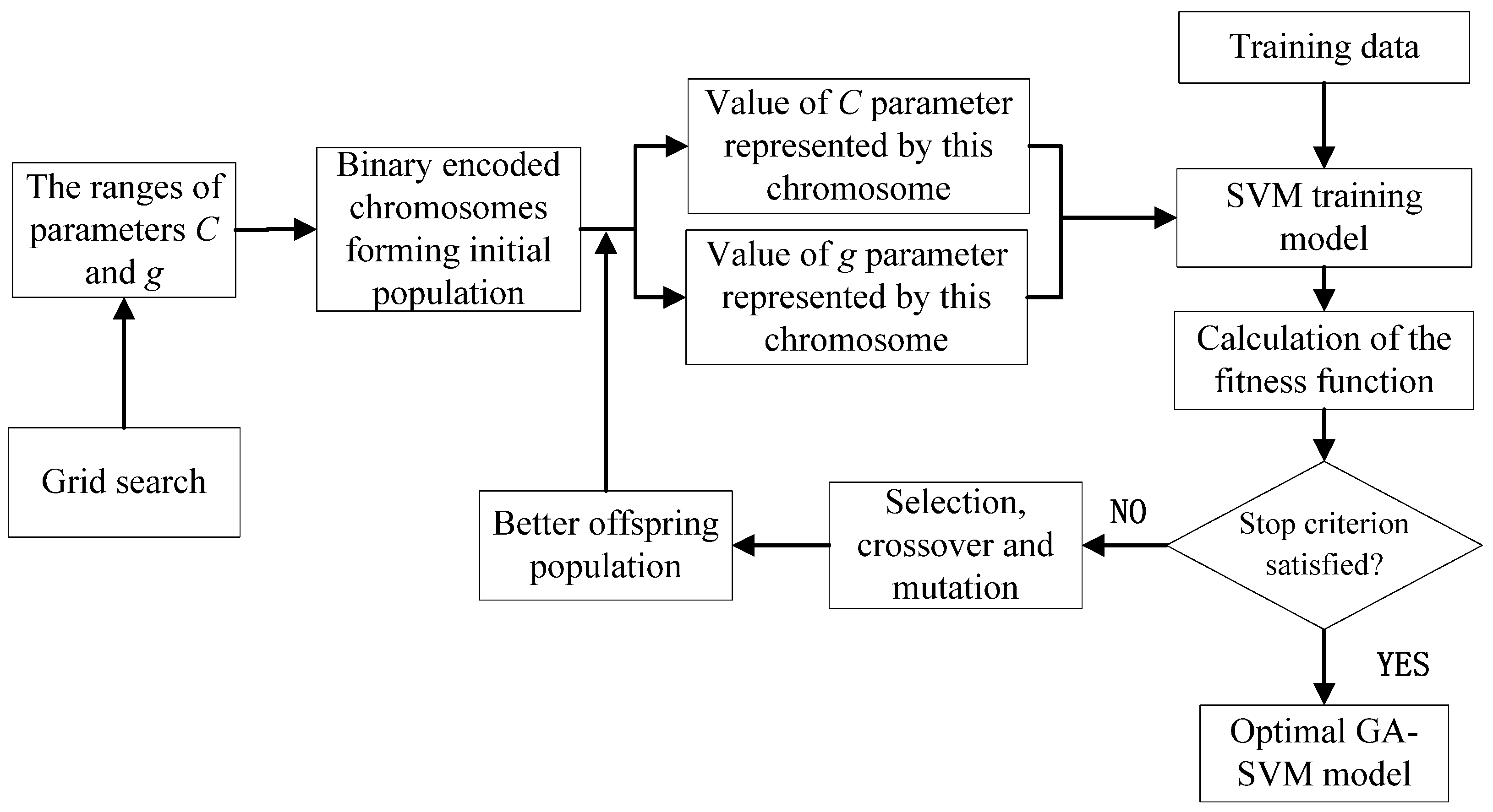
2.4. Model Parameter Optimization with Grid Search and GA
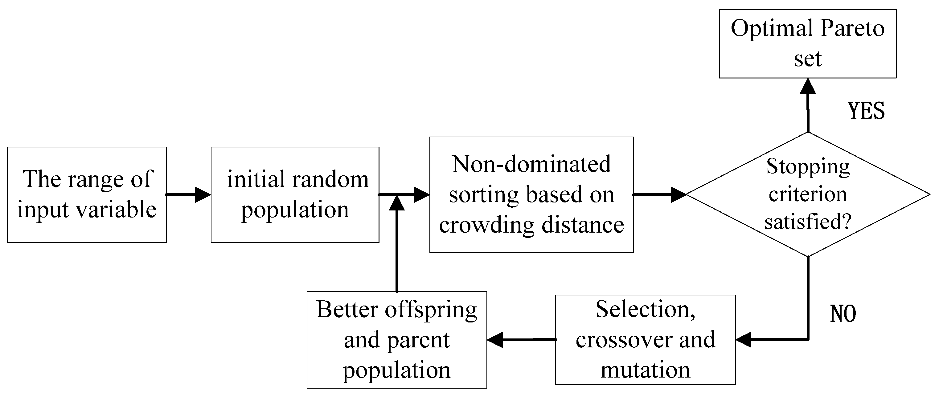
2.5. Multi-Objective Optimization
3. Results and Discussion
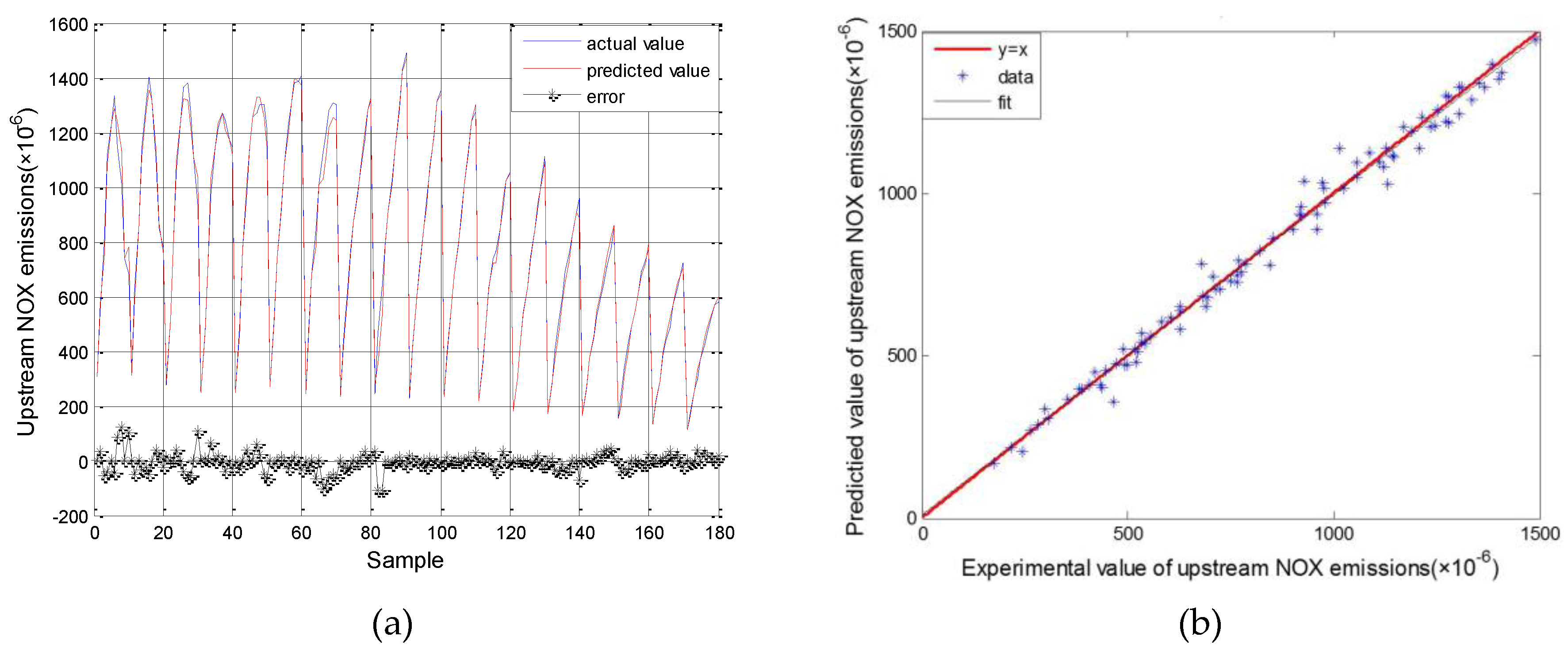
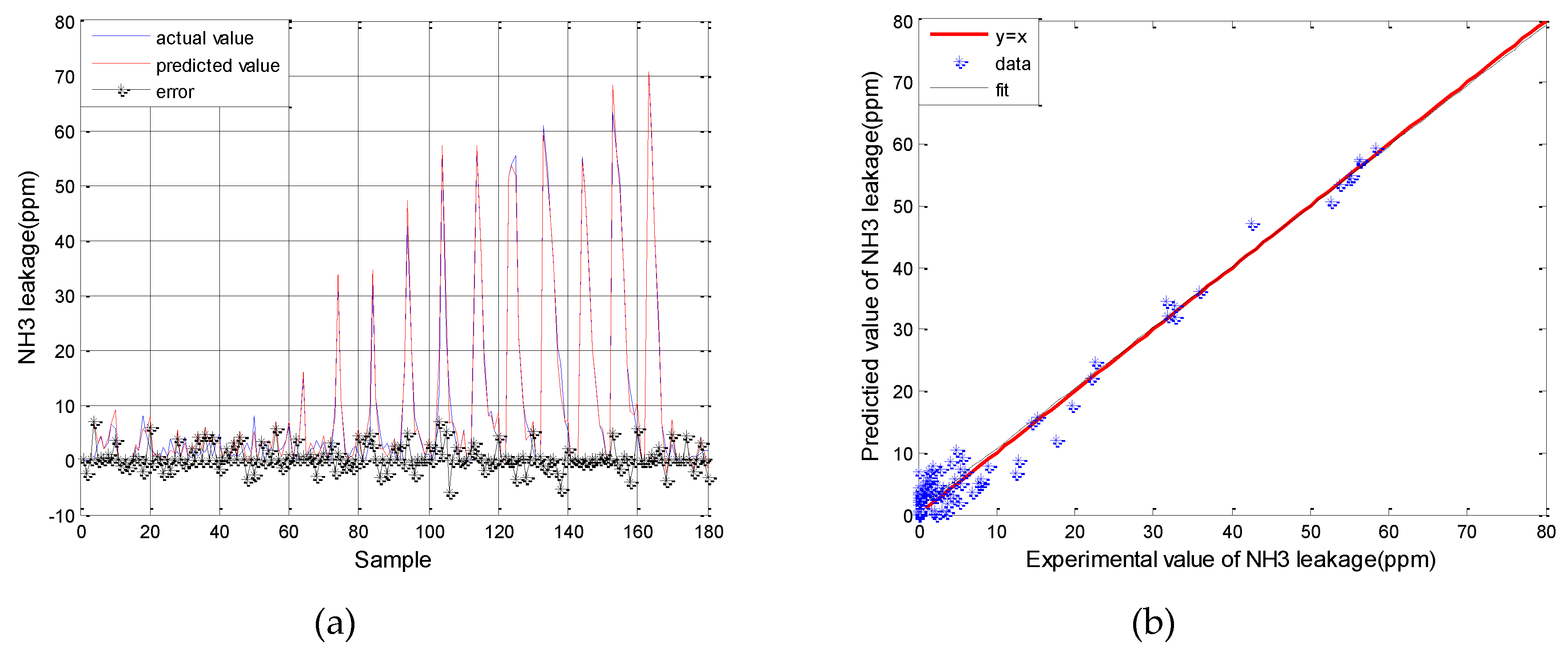
3.1. Results for SVM Model Simulation
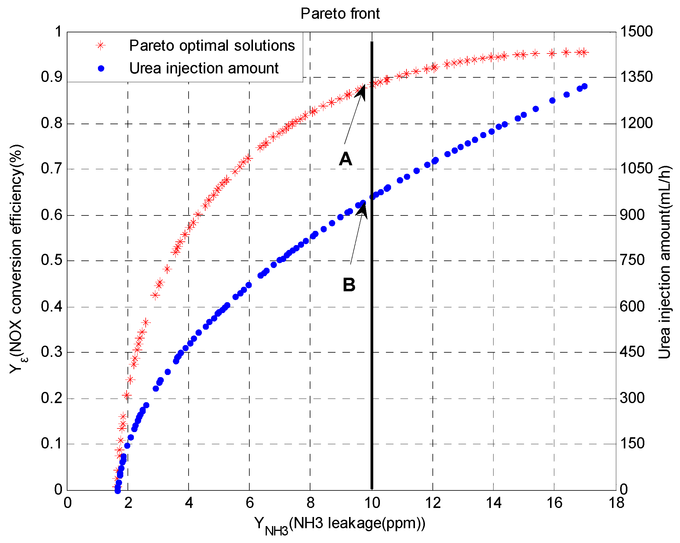
3.2. NSGA-II Multi-Objective Optimization Results
4. Conclusions
- (1)
- The prediction accuracy of the engine and SCR models could be improved by using an SVM, the parameters of which were optimized using a GA. The RMSE of upstream and downstream NOx emissions and NH3 slip for the all datasets was 44.01 × 10⁻⁶, 21.87 × 10⁻⁶ and 2.22 × 10⁻⁶, respectively. The MAPE of the models were all under 5%, and was good enough for estimating the actual outputs.
- (2)
- The optimized urea injection amounts under certain operating points were obtained through multi-objective genetic algorithm for maximizing NOx conversion efficiency while minimizing NH3 slip.
Acknowledgments
Author Contributions
Conflicts of Interest
References
- Brookshear, D.W.; Nguyen, K.; Toops, T.J.; Bunting, B.G.; Rohr, W.F. Impact of Biodiesel-Based Na on the Selective Catalytic Reduction of NOx by NH3 over Cu–Zeolite Catalysts. Top. Catal. 2013, 56, 62–67. [Google Scholar] [CrossRef]
- Chen, P.; Wang, J. Nonlinear and adaptive control of NO/NO2 ratio for improving selective catalytic reduction system performance. J. Eng. Marit. Environ. 2007, 221, 31–42. [Google Scholar] [CrossRef]
- Iwasaki, M.; Shinjoh, H. A comparative study of “standard”, “fast” and “NO2” SCR reactions over Fe/zeolite catalyst. Appl. Catal. A Gen. 2010, 390, 71–77. [Google Scholar] [CrossRef]
- Forzatti, P. Present status and perspectives in de-NOx SCR catalysis. Appl. Catal. A Gen. 2001, 222, 221–236. [Google Scholar] [CrossRef]
- Koebel, M.; Elsener, M.; Madia, G. Recent Advances in the Development of Urea-SCR for Automotive Applications; SAE International: Warrendale, PA, USA, 2001. [Google Scholar]
- Majd, E.; Shamekhi, A.H. Development of a neural network model for selective catalytic reduction (SCR) catalytic converter and ammonia dosing optimization using multi objective genetic. Chem. Eng. J. 2010, 165, 508–516. [Google Scholar]
- Beale, A.M.; Lezcano-Gonzalez, I.; Maunula, T.; Palgrave, R.G. Development and characterization of thermally stable supported V–W–TiO2 catalysts for mobile NH3–SCR applications. Catal. Struct. React. 2015, 1, 25–34. [Google Scholar] [CrossRef]
- Karimi, H.R.; Zhang, H.; Zhang, X.; Wang, J.; Chadli, M. Control and Estimation of Electrified Vehicles. J. Frankl. Inst. 2015, 352, 421–424. [Google Scholar] [CrossRef]
- Ardanese, R.; Ardanese, M.; Besch, M.C.; Adams, T.; Thiruvengadam, A.; Shade, B.C.; Gautam, M.; Oshinuga, A.; Miyasato, M. Development of an Open Loop Fuzzy Logic Urea Dosage Controller for Use With an SCR Equipped HDD Engine. In Proceedings of ASME 2009 Internal Combustion Engine Division Fall Technical Conference, Lucerne, Switzerland, 27–30 September 2009; pp. 353–363.
- Hu, J.; Zhao, Y.; Zhang, Y.; Shuai, S. Development of Closed-Loop Control Strategy for Urea-SCR Based on NOx Sensors; SAE Technical Paper; SAE International: Warrendale, PA, USA, 2011. [Google Scholar]
- Willems, F.; Cloudt, R. Experimental demonstration of a new model-based SCR control strategy for cleaner heavy-duty diesel engines. IEEE Trans. Control Syst. Technol. 2011, 19, 1305–1313. [Google Scholar] [CrossRef]
- Willems, F.; Cloudt, R.; van den Eijnden, E.; van Genderen, M. Is Closed-Loop SCR Control Required to Meet Future Emission Targets? SAE International: Warrendale, PA, USA, 2007. [Google Scholar]
- Herman, A.; Wu, M.; Cabush, D.; Shost, M. Model based control of SCR dosing and OBD strategies with feedback from NH3 sensors. SAE Int. J. Fuels Lubr. 2009, 2, 375–385. [Google Scholar] [CrossRef]
- Zambrano, D.; Tayamon, S.; Carlsson, B.; Wigren, T. Identification of a discrete-time nonlinear Hammerstein-Wiener model for a selective catalytic reduction system. In Proceedings of the American Control Conference (ACC), San Francisco, CA, USA, 29 June–1 July 2011.
- Surenahalli, H.S.; Parker, G.; Johnson, J.H. Extended Kalman Filter Estimator for NH3 Storage, NO, NO2 and NH3 Estimation in a SCR; SAE Technical Paper; SAE International: Warrendale, PA, USA, 2013. [Google Scholar]
- D Ambrosio, S.; Finesso, R.; Fu, L.; Mittica, A.; Spessa, E. A control-oriented real-time semi-empirical model for the prediction of NOx emissions in diesel engines. Appl. Energy 2014, 130, 265–279. [Google Scholar] [CrossRef]
- Asprion, J.; Chinellato, O.; Guzzella, L. A fast and accurate physics-based model for the NOx emissions of Diesel engines. Appl. Energy 2013, 103, 221–233. [Google Scholar] [CrossRef]
- Maroteaux, F.; Saad, C. Combined mean value engine model and crank angle resolved in-cylinder modeling with NOx emissions model for real-time Diesel engine simulations at high engine speed. Energy 2015, 88, 515–527. [Google Scholar] [CrossRef]
- Lv, Y.; Yang, T.; Liu, J. An adaptive least squares support vector machine model with a novel update for NOx emission prediction. Chemom. Intell. Lab. Syst. 2015, 145, 103–113. [Google Scholar] [CrossRef]
- Taghavifar, H.; Mardanib, A.; Mohebbib, A.; Khalilaryaa, S.; Jafarmadara, S. Appraisal of artificial neural networks to the emission analysis and prediction of CO2, soot, and NOx of n-heptane fueled engine. J. Clean. Prod. 2016, 112, 1729–1739. [Google Scholar] [CrossRef]
- Lv, Y.; Liu, J.; Yang, T.; Zeng, D. A novel least squares support vector machine ensemble model for NOx emission prediction of a coal-fired boiler. Energy 2013, 55, 319–329. [Google Scholar] [CrossRef]
- Vapnik, V.N.; Vapnik, V. Statistical Learning Theory; Wiley New York: New York, NY, USA, 1998; Volume 1. [Google Scholar]
- Martínez-Morales, J.D.; Palacios-Hernández, E.R.; Velázquez-Carrillo, G.A. Modeling and multi-objective optimization of a gasoline engine using neural networks and evolutionary algorithms. J. Zhejiang Univ. Sci. A 2013, 14, 657–670. [Google Scholar] [CrossRef]
- D Errico, G.; Cerri, T.; Pertusi, G. Multi-objective optimization of internal combustion engine by means of 1D fluid-dynamic models. Appl. Energy 2011, 88, 767–777. [Google Scholar] [CrossRef]
- Shin, K.; Lee, T.S.; Kim, H. An application of support vector machines in bankruptcy prediction model. Expert Syst. Appl. 2005, 28, 127–135. [Google Scholar] [CrossRef]
- Vapnik, V.N. The Nature of Statistical Learning Theory. IEEE Trans. Neural Netw. 1995, 10, 988–999. [Google Scholar] [CrossRef] [PubMed]
- Severyn, A.; Moschitti, A. Large-Scale Support Vector Learning with Structural Kernels. Lect. Notes Comput. Sci. 2010, 6323, 229–244. [Google Scholar]
- Tong, H.; Chen, D.R.; Yang, F. Learning Rates for -Regularized Kernel Classifiers. J. Appl. Math. 2013, 2013, 1–11. [Google Scholar] [CrossRef]
- Dibike, Y.B.; Velickov, S.; Solomatine, D.; Abbott, M. Model Induction with Support Vector Machines: Introduction and Applications. J. Comput. Civ. Eng. 2001, 15, 208–216. [Google Scholar] [CrossRef]
- Smola, A.J. Learning with kernels | Support Vector Machines. Lect. Notes Comput. Sci. 2008, 42, 1–28. [Google Scholar]
- Goldberg, D.E. Genetic Algorithms in Search Optimization and Machine Learning; Addison-Wesley Professional: Boston, MA, USA, 1989; Volume 412. [Google Scholar]
- Goldberg, D.E. Genetic Algorithms; Pearson Education: Upper Saddle River, NJ, USA, 2006. [Google Scholar]
- Chen, R.; Sun, D.-Y.; Qin, D.-T.; Luo, Y.; Hu, F.-B. A novel engine identification model based on support vector machine and analysis of precision-influencing factors. J. Cent. South Univ.: Sci. Technol. 2010, 41, 1391–1397. [Google Scholar]
- Zhou, H.; Zhao, J.P.; Zheng, L.G.; Wang, C.L.; Cen, K.F. Modeling NOx emissions from coal-fired utility boilers using support vector regression with ant colony optimization. Eng. Appl. Artif. Intell. 2012, 25, 147–158. [Google Scholar] [CrossRef]
- Deb, K. Multi-Objective Optimization Using Evolutionary Algorithms; John Wiley & Sons: New York, NY, USA, 2001; Volume 16. [Google Scholar]
- Knowles, J.; Corne, D. The pareto archived evolution strategy: A new baseline algorithm for pareto multiobjective optimization. In Proceedings of the 1999 Congress on Evolutionary Computation, 1999, Washington, DC, USA, 6–9 July 1999.
- Zitzler, E. Evolutionary Algorithms for Multiobjective Optimization: Methods and Applications; ETH Zurich: Zürich, Switzerland, 1999. [Google Scholar]
- Coello, C.A.; Christiansen, A.D. Multiobjective optimization of trusses using genetic algorithms. Comput. Struct. 2000, 75, 647–660. [Google Scholar] [CrossRef]
- Osyczka, A. Multicriteria optimization for engineering design. Des. Opt. 1985, 1, 193–227. [Google Scholar]


| Features | Parameters |
|---|---|
| Engine type | YUCHAI YC6L-42 |
| Number of cylinder | 6 |
| Displacement volume | 6.6 L |
| Max. power | 179 kW |
| Max. torque | 940 N·m |
| Cooling system | Water-cooled |
| Equipment | Measurement Parameters |
|---|---|
| Eddy current dynamometer | Speed, torque |
| CAN bus | circulating oil |
| AVL4000 | NOx emissions |
| LDS6 | NH3 slip |
| Mode | Speed (rpm) | Torque (N*m) | Load (%) | Fuel Supply (mg/cyc) | Temperature of Catalyst (°C) | Upstream NOx (ppm) |
|---|---|---|---|---|---|---|
| 1 | 1000 | 215 | 30 | 171 | 215 | 862 |
| 2 | 1000 | 391 | 60 | 309 | 326 | 1401 |
| 3 | 1000 | 585 | 90 | 503 | 492 | 849 |
| 4 | 1500 | 204 | 30 | 168 | 250 | 684 |
| 5 | 1500 | 408 | 60 | 300 | 344 | 1131 |
| 6 | 1500 | 612 | 90 | 436 | 415 | 1306 |
| 7 | 2000 | 201 | 30 | 178 | 249 | 498 |
| 8 | 2000 | 395 | 60 | 299 | 318 | 767 |
| 9 | 2000 | 596 | 90 | 429 | 394 | 1026 |
| 10 | 2500 | 153 | 30 | 165 | 227 | 290 |
| 11 | 2500 | 312 | 60 | 265 | 296 | 489 |
| 12 | 2500 | 471 | 90 | 364 | 378 | 674 |
| Model | Upstream NOx Emissions | Downstream NOx Emissions | NH3 Slip | ||||||
|---|---|---|---|---|---|---|---|---|---|
| Training | Test | All | Training | Test | All | Training | Test | All | |
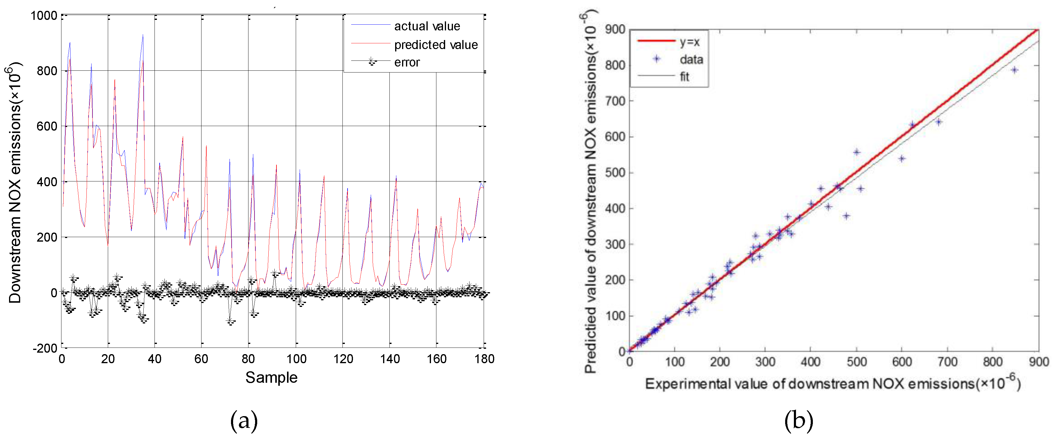
| RMSE(ppm) | 24.62 | 57.16 | 44.01 | 19.56 | 25.87 | 21.87 | 1.34 | 2.84 | 2.22 |
| MAPE(%) | 1.71 | 4.77 | 3.24 | 2.17 | 6.89 | 4.53 | - | - | - |
| R2 | 0.99 | 0.98 | 0.99 | 0.99 | 0.98 | 0.99 | 0.99 | 0.97 | 0.98 |
| Fits | Y1 = 0.9849 × X1 + 8.0395 | Y2 = 0.9644 × X2 + 6.8769 | Y3 = 0.9786 × X3 + 0.9270 | ||||||
| Model | Inputs | Outputs |
|---|---|---|
| M1 | Speed, Torque, Fuel supply pre cycle | Upstream NOx emissions |
| M2 | Temperature, Upstream NOx emissions, urea injection amount | Downstream NOx emissions |
| M3 | Temperature, Upstream NOx emissions, urea injection amount | NH3 slip |
| Model | Speed (rpm) | Torque (N*m) | Temperature °C | Upstream NOx (ppm) | Urea Injection Amount (mL/h) | NOx Conversion Efficiency (%) | NH3 Slip (ppm) |
|---|---|---|---|---|---|---|---|
| 4 | 1500 | 204 | 250 | 684 | 940 | 88 | 9.7 |
| 5 | 1500 | 408 | 344 | 1131 | 1256 | 90 | 9.8 |
| 6 | 1500 | 612 | 415 | 1306 | 1553 | 90 | 9.6 |
| 7 | 2000 | 201 | 249 | 498 | 698 | 91 | 9.4 |
| 8 | 2000 | 395 | 318 | 767 | 1468 | 87 | 9.6 |
| 9 | 2000 | 596 | 394 | 1026 | 1178 | 92 | 9.3 |
© 2016 by the authors; licensee MDPI, Basel, Switzerland. This article is an open access article distributed under the terms and conditions of the Creative Commons Attribution (CC-BY) license (http://creativecommons.org/licenses/by/4.0/).
Share and Cite
Liu, B.; Yan, F.; Hu, J.; Turkson, R.F.; Lin, F. Modeling and Multi-Objective Optimization of NOx Conversion Efficiency and NH3 Slip for a Diesel Engine. Sustainability 2016, 8, 478. https://doi.org/10.3390/su8050478
Liu B, Yan F, Hu J, Turkson RF, Lin F. Modeling and Multi-Objective Optimization of NOx Conversion Efficiency and NH3 Slip for a Diesel Engine. Sustainability. 2016; 8(5):478. https://doi.org/10.3390/su8050478
Chicago/Turabian StyleLiu, Bo, Fuwu Yan, Jie Hu, Richard Fiifi Turkson, and Feng Lin. 2016. "Modeling and Multi-Objective Optimization of NOx Conversion Efficiency and NH3 Slip for a Diesel Engine" Sustainability 8, no. 5: 478. https://doi.org/10.3390/su8050478
APA StyleLiu, B., Yan, F., Hu, J., Turkson, R. F., & Lin, F. (2016). Modeling and Multi-Objective Optimization of NOx Conversion Efficiency and NH3 Slip for a Diesel Engine. Sustainability, 8(5), 478. https://doi.org/10.3390/su8050478