The Combination of Expert Judgment and GIS-MAIRCA Analysis for the Selection of Sites for Ammunition Depots

Abstract

This paper suggests spatial multi-criteria model in order to assist decision makers in the selection of sites which are suitable for ammunition depots (AD). They represent military facilities which have more criteria that need to be matched than civil structures. The proposed model is based on combined use of Geographic information systems (GIS) and multi-criteria techniques. The model application is presented in the case study of Carpathian region, the Eastern part of Serbia. The model deals with nine restrictions and six evaluation criteria. Decision Making Trial and Evaluation Laboratory—Analytic Network Process (DEMATEL-ANP) multi-criteria techniques are used to determine weight coefficients of evaluation criteria. Along with the above mentioned methods, this paper introduces a new technique for the multi-criteria decision making—MAIRCA (MultiAttributive Ideal-Real Comparative Analysis) method. The MAIRCA method is used for the ranking and selection of suitable locations. The results have shown that 45 km² of the Carpathian region is very suitable for ammunition depot construction. The MAIRCA method chose location L1 as the most appropriate. Sensitivity analysis shows that the model is capable of identifying a suitable ammunition depot location. This approach can be helpful in determining suitable ammunition depot locations in other regions with similar geographic conditions and can also be successfully used for the suitability assessment of existing ammunition depots.

1. Introduction

In recent years, much effort has been made to solve facility location problems (FLP). Furthermore, many additional features have been comprised in location models including multiple objectives and multiple facility types. Facility location problems continue to be an important part of strategic planning and decision making for logistic managers today. FLP should identify the best set of storage locations with the best mix of munitions’ inventories that considers transportation and other logistical restrictions in satisfying a set of potential demands [1]. The majority of the research in this area has been related to the problem of where to locate municipal facilities. However, several references are used to identify adequate locations for military related facilities that store munitions around the world [2,3,4,5,6,7,8,9].

Numerous Unplanned Explosions at Munitions Sites (UEMS) attract progressively more public attention due to the existing risk built from inadequate management of explosive materiel and its storage at the unsafe locations. UEMS leave behind numerous direct and indirect consequences. Along with the casualties and severely damaged buildings, there are additional expenses in medical care, reconstruction and rebuilding costs, unexploded ordnance removal costs, harmful impact on the environment and business profits loss. [10].

In 2006, in the Serbian army ammunition depot (AD) near Paraćin town, a huge explosion occurred, supposedly due to the inappropriate storage of ammunition. The explosion directly resulted in the total destruction of stored ammunition, the injury of 23 people, the pollution of the surrounding 30 square kilometers with nearly 90,000 unexploded ordnance items, the damage and demolition of 600 objects and 12 schools, and glass breakage in around 4740 buildings in the Paraćin town and around 2000 buildings in the nearby town of Ćuprija. Broader socioeconomic concerns were evident with the temporary highway and railroad shutting down and the evacuation of people from the nearby locations [11]. These facts clearly point out the essential need to locate and build ammunition depots at safer locations, without losing their functional purposes.

The scope of this paper points to the wider public necessity for locating and building ammunition depots according to the legislations and law in order to establish safe surroundings and to preserve the environment. Therefore, finding suitable locations for ammunition depots is rather a complex issue requiring careful, joint analysis of numerous criteria.

Optimum selection of ammunition depot locations requires consolidation of mutually opposed economic and technical factors with ecological and safety restrictions. In other words, decision makers (DM) are confronted with a dual challenge. They have to satisfy the technological requirements of building AD while taking into account the economic aspects. Furthermore, it is needed to minimize risk to the environment and to meet location safety standards. In order to do this, it is necessary to set certain rules which will help DMs to evaluate different locations based on certain spatial, safety, environmental and economic criteria and restrictions.

Geographic information technologies (GIS) are ideal for this kind of studies because they can efficiently manage large numbers of spatial and attributive data collected from various sources. GIS have certain flaws when used for location selection, like the lack of multi-criteria decision making (MCDM) possibilities and optimum location recommendations. It is essential to combine tools for MCDM with GIS in order to obtain MCDM as well as spatial outputs. The combination of GIS and multi-criteria decision analysis (MCDA) is a widely accepted concept for spatial problem solving in many areas such as the environment, ecology, transportation, urban and regional planning, waste management, hydrology, agriculture, forestry, geology and site selection [12].

GIS-MCDA is currently the most advantageous concept used to assist DM in selecting the optimal choice from a number of feasible options/alternatives with multiple choice criteria and diverse criterion priorities. The multi-criterion choice can be attributed to spatial decision-making problems involving the search for the optimal AD site. Similar problems, often analyzed in GIS, include site selection for critical ecologically sensitive areas, hazardous waste disposal sites and emergency service locations [13,14,15,16,17,18,19]. A large number of studies combine GIS with different MCDM: AHP [20,21], ANP [22,23], TOPSIS [24,25], PROMETHEE [26,27], VIKOR [28,29], etc. This paper presents the GIS-MAIRCA approach, thus investigating the new MCDM method and its potential use with GIS for the AD location problem. This paper comprises of the following parts: Definition of aim/problem and model structure; Identification of restrictions and evaluation criteria; Data gathering and building of the spatial criteria basis; GIS-MCDA evaluation; Sensitivity analysis and GIS visualization of the final solutions and recommendations.

2. Methodological Background

The methodological hierarchy model presented in this paper is based on spatial MCDA structure. Spatial multi-criteria decision analysis (SMCDA) consists of a number of procedures including the use of geographic data and DM preferences, and the manipulation of data and preferences according to specified decision rules [12]. This approach uses the capabilities of GIS in spatial data management and the flexibility of MCDA to combine factual information (e.g., terrain slope, road and railways, land cover/use, etc.) with value-based information (e.g., expert assessments, standards, opinion polls, etc.) [30]. The main advantage of GIS and MCDA integration is the ability to obtain unique capabilities which are complementary to each other. GIS has great possibilities for the manipulation, storage, management, analysis and visualization of geospatial data while MCDA offers an assortment of procedures, techniques and algorithms for decision making structure and design, and evaluating and prioritizing options [31].

From a methodological point of view, the suggested model for defining suitable locations for AD consists of the following steps (Figure 1):

2.1. Definition of Aim/Problem and Model Architecture

Identification of suitable AD locations is the general aim of this paper. DM must justify their choice regarding AD location selection through a multisystem, transparent and documented process. The building of network hierarchy models involves an important creative phase in the problem solving process because the consideration of all relevant factors and their mutual interactions is the key to obtaining the correct solution.

The MCDA model is suggested as a relevant option for systematic analysis and rational decision making due to the complexity of the location selection problem. The MCDA model is based on the joint use of GIS and multi-criteria techniques such as DEMATEL, ANP and MAIRCA.

Authors have chosen the hybrid DEMATEL-ANP model because it eliminates subjectivity while generating model architecture, unlike the classic ANP method. The DEMATEL method creates a cause and effect diagram based on a mathematic formulation. Further on, this relationship is used as an initial data set for the ANP method. This paper also presents a novel MCDM method—MAIRCA. This method is proven to be more stable than other methods, like TOPSIS or ELECTRE. One reason is the different criteria normalization. In [32], it was shown that methods using a linear model of input data normalization have greater stability and rank consistently during sensitivity analysis. The MAIRCA method uses a linear normalization model. The second reason for choosing the MAIRCA method is its simple mathematic apparatus, solution stability and the possibility to combine this method with other ones [32].

2.2. Identification of Restrictions and Evaluation Criteria

The location selection process is a MCDA problem requiring adequate consideration of the comprehensive criteria set in order to determine the suitability of certain areas for a particular land use. The MCDA process uses two criteria categories: restrictions and evaluation criteria. Restrictions are based on the criteria which limit (exclude) possible alternatives and that are based on Boolean relations (true/false). The evaluation criteria can be quantified according to the degree of suitability for all feasible alternatives [33,34]. Criteria for the assessment of AD location suitability were adopted according to the established goals and based on UN and national regulations along with the leading military publications and literature [35,36,37,38,39,40,41]. They comprise the following factors: technical, safety, environmental, spatial and socioeconomic. In order to determine restriction criteria, it is necessary to study the territory status carefully (settlements, roads, rivers, protected areas, etc.), along with the regulations (European, national, regional and local) and further determine the boundary values which will exclude some alternatives from the future analysis.

2.3. Data Gathering and Building of the Spatial Criteria Basis

It is necessary, during this step, to form individual map layers which correspond to each identified restriction and evaluation criteria. This can be achieved by different GIS operations used to enter, accept and transform spatial and thematic data into digital forms (map overlay, buffering, distance mapping, etc.). Initial data mainly come from digital and analog cartographic documents, terrain images, blueprints, statistic reports, etc. GIS data criteria are usually organized in vector or rasterized format. Successive arithmetic operations in GIS (reclassification, overlay functions, Boolean algebra, etc.) criteria maps are converted to the rasterized format, where every raster cell presents an alternative towards the goal. Calculations based on rasterized data formats are far less complicated than those on vector data [42].

2.4. GIS-MCDA Evaluation

This phase concerns standardization and evaluation of all criteria used in the analysis.

2.4.1. Formation and Aggregation of Restrictions Map

The implementation of restrictions in the thematic maps is accomplished using Boolean (logical) algebra, in the way that raster cells (alternatives) for the excluded area have zero value (0), while the other alternatives are given a value of one (1). The final constrained area is obtained through aggregation of all layers (criteria) with restrictions. Only the locations which are suitable on all restriction levels in the restrictions map can be considered as a potential location for the construction of AD and therefore are the subject of further analysis.

2.4.2. Individual Assessment of Evaluation Criteria and Standardization

Criteria are presented on maps in GIS layers in various ways and in various forms. The method of weighted linear combination (WLC) requires that all data criteria is standardized [33] or transformed (reclassified) into mutually comparable units. There are many useful approaches that can be used so the attributive layers are comparable [31]. The decision as to which approach should be applied depends on the attribute nature and on DM. The most frequently used approach is linear transformation, or transformation on the interval scale, when every raster cell (attribute) gets a nondimensional value x_i on the adopted scale in terms of the aim of the analysis. Hence, every attribute acquires an integer value x_i according to the class i association. It is common in this method to determine the midpoint of the attribute interval because it represents the boundary between the desirable and undesirable solution. In real conditions, this method gives very good results even though it is quite arbitrary.

2.4.3. Comparison and Relative Assessment of Criteria Weight (DEMATEL-ANP)

While solving real problems, criteria do not have the same degree of significance so the DM has to define significance factors for some criteria using weighting coefficients (weights) or criteria evaluation. The WLC method demands normalized weights, meaning that the sum of all weights must be 1.

DEMATEL and ANP (DANP) method is used for the calculation of normalized criteria weights followed then by WLC method. The DEMATEL method was originally developed by the Science and Human Affairs Program of the Battelle Memorial Institute of Geneva, with the purpose of studying a complex and intertwined problem [43]. 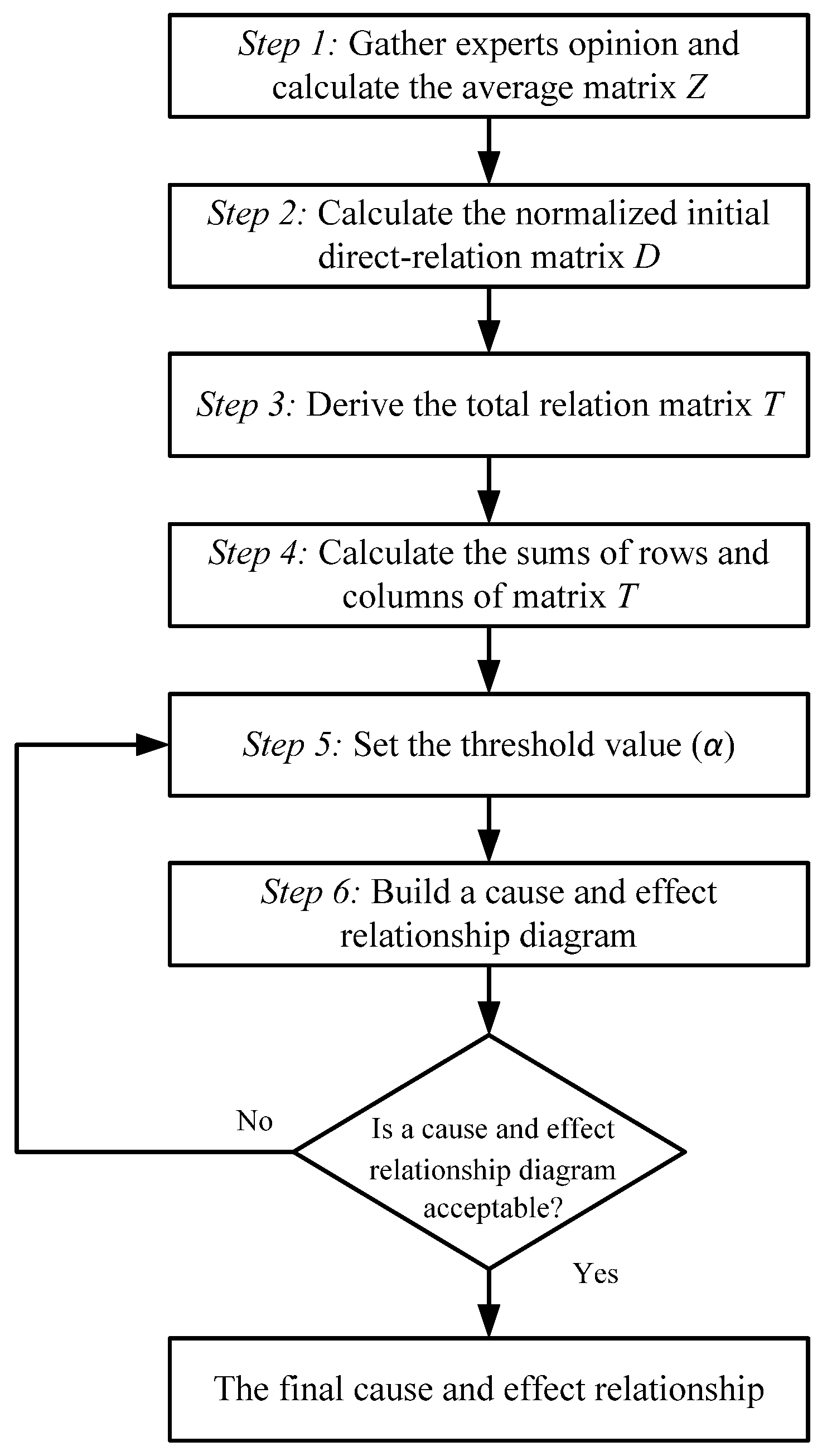It has been widely accepted as one of the best tools to solve the cause and effect relationship among evaluation criteria [43,44,45,46,47]. The original DEMATEL method is modified by some researchers so as to make it comply with their problems. The modified DEMATEL method which is used in this paper is adapted from the study of [48] (Figure 2).

The full procedure of the previously defined DEMATEL method is explained as follows:

Step 1. Gather experts’ opinions and calculate the average matrix Z. The modified DEMATEL method is built first creating the direct-relation matrix Z where Z is (n × n) matrix, n represents the number of criteria. The direct relation matrices are all obtained by holding a pair-wise comparison among the criteria themselves in which Z_ij indicates the degree to which the criterion $C_i$ affects criterion $C_j$. Therefore, the relationship among the criteria could be held within a matrix. In this method, the effects of the criteria on each other are expressed in terms of linguistic equations.

A group of e experts and n factors are used in this step. Each expert is asked to view the degree of direct influence between two factors based on a pair-wise comparison. The degree to which the expert perceived factor i impacts factor j is denoted as $z_{ij}$. For each expert, a n × n non-negative matrix is constructed (n represents the number of criteria) as $Z^e=\left[z_{ij}^e\right]$, where e is the expert number of participating in evaluation process with 1 ≤ e ≤ k. Thus, $Z^1,Z^2,\mathrm{...},Z^k$ are the matrices from m experts. In this method, the effects of the criteria on each other are expressed in terms of linguistic equations. Aggregation of experts’ opinions gives the final matrix $Z=\left[z_{ij}\right]$

$$z_{ij}=\sqrt[k]{{\displaystyle \prod _{i=1}^k{z}_{ij}^e}}$$

(1)

where $z_{ij}^e$ denotes preference of expert number e, k is total number of experts.

Step 2. Calculate the normalized initial direct-relation matrix D. The normalized initial direct-relation matrix $D=\left[d_{ij}\right]$, where value of each element in matrix D is ranged between [0,1]. The calculation is shown below.

$$D=\left[\begin{array}{cccc}{d}_{11}& d_{12}& \mathrm{...}& d_{1n}\\ d_{21}& d_{22}& \mathrm{...}& d_{2n}\\ \mathrm{...}& \mathrm{...}& \mathrm{...}& \mathrm{...}\\ d_{n1}& d_{n2}& \mathrm{...}& d_{nn}\end{array}\right]$$

(2)

where the elements of the initial direct-relation matrix is calculated from

$$d_{ij}=\frac{z_{ij}}{R}$$

(3)

$$R=\max \left({\displaystyle {\sum }_{j=1}^n{z}_{ij}}\right)$$

(4)

where n denotes total number of criteria.

Step 3. Derive the total relation matrix T. The total-influence matrix T is obtained by utilizing Equation (7), in which, I is an n × n identity matrix. The element of t_ij represents the indirect effects that factor i had on factor j, then the matrix T reflects the total relationship between each pair of system factors. Initial normalized direct-relation matrix can be separated into separate sub matrices i.e., ($D_1$,$D_2$,$D_3$). It was proven that

$${\lim }_{k\to \propto }{\left(D_s\right)}^w=0$$

(5)

And

$${\lim }_{k\to \propto }\left(I+D_s+\mathrm{...}+D_s^2+\mathrm{...}+D_s^k\right)={\left(I-D_s\right)}^{-1}$$

(6)

where 0 is the null matrix and I is the identity matrix [49,50]. Therefore, the total-relation matrix T can be acquired by calculating the following term [51]:

$$T=\underset{w\to \propto }{\lim }\left(D+D^2+\mathrm{...}+D^w\right)=D{\left(I-D\right)}^{-1}$$

(7)

As it is previously shown, the total relation matrix for the criteria (T) can be presented as:

$$T=\left[\begin{array}{cccc}{t}_{11}& t_{12}& \mathrm{...}& t_{1n}\\ t_{21}& t_{22}& \mathrm{...}& t_{2n}\\ \mathrm{...}& \mathrm{...}& \mathrm{...}& \mathrm{...}\\ t_{n1}& t_{n2}& \mathrm{...}& t_{nn}\end{array}\right]$$

(8)

where t_ij is the overall influence rating of decision maker for each alternative $i$ against criterion $j$.

Step 4. Calculate the sums of rows and columns of matrix T. The sum of rows and sum of columns of the sub-matrices $T_1$, $T_2$ and $T_3$ denoted by the numbers D_i and R_i, respectively, can be obtained through Equations (9) and (10), respectively:

$$D_i={\displaystyle {\sum }_{i=1}^n{t}_{ij}},i=1,2,\mathrm{...},n$$

(9)

$$R_i={\displaystyle {\sum }_{j=1}^m{t}_{ij}},j=1,2,\mathrm{...},m$$

(10)

where n denotes number of criteria.

Step 5. Determination of the threshold value α. Threshold value α is used for creating a cause and effect relationship diagram. Threshold value α is calculated as the median of elements (t_ij) from the matrix T, according to Equation (11). This calculation aims eliminate some minor effects of elements in matrix T [52].

$$\alpha =\frac{{\displaystyle {\sum }_{i=1}^n{\displaystyle {\sum }_{j=1}^n{t}_{ij}}}}{N}$$

(11)

where N is the total number of elements in matrix T.

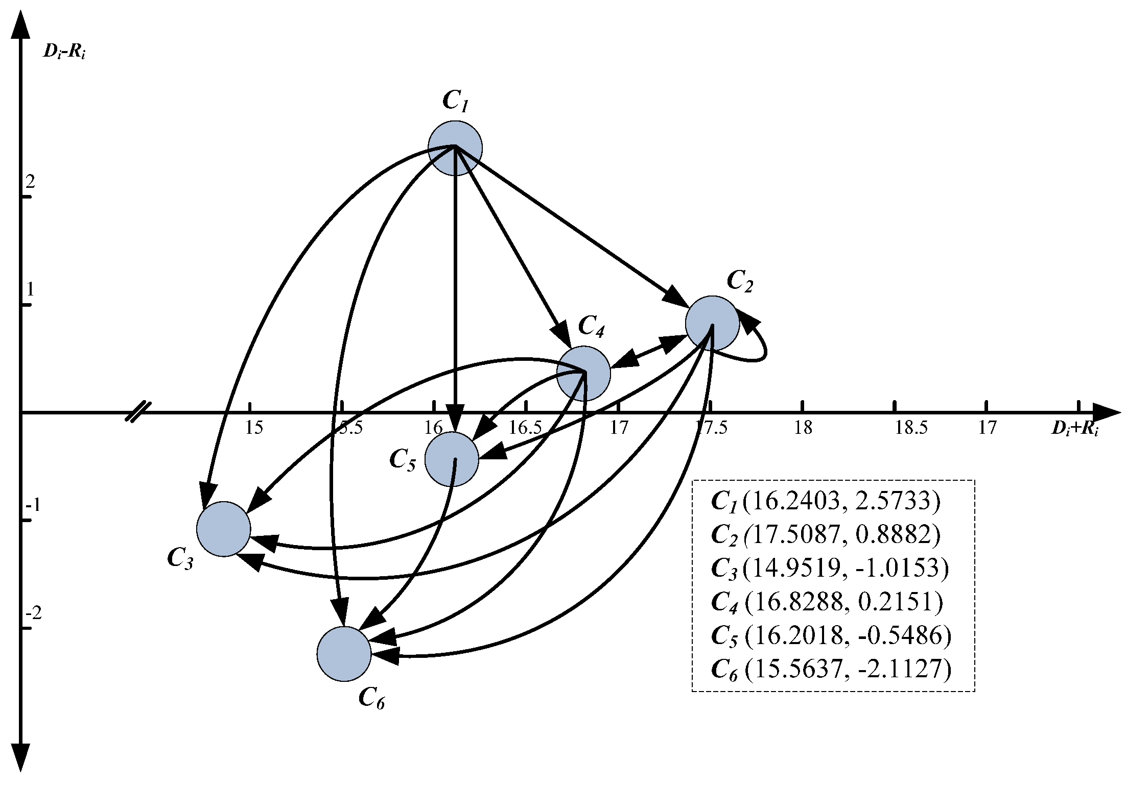
Step 6. Creating a cause and effect relationship diagram. The cause and effect diagram is constructed by mapping all coordinate sets of (D_i + R_j, D_i − R_j) to visualize the complex interrelationship and provide information in order to determine the most important factors and how they influence the affected factors [53]. The factors t_ij that are greater than α are selected and shown in the cause and effect diagram [52].

After designing the cause and effect relationship diagram, weighted coefficients of criteria are calculated using the ANP method in the next phase. Afterwards, the implementation of DEMATEL method into the ANP method is elaborated.

The ANP method was developed to avoid the hierarchical restrictions that exist in the AHP method [54]. ANP presents a generalized AHP method, designed so that the hierarchy is replaced by a network. The ANP method, unlike hierarchy structured problems, takes into account different forms of dependency and feedback. The structure of the feedback is not linear and is more close to the network where interdependent loops frequently appear. The calculation of relative weights of criteria using traditional ANP means the levels of interdependence of factors are treated as reciprocal values. On the contrary, using the DEMATEL method, the levels of interdependence of factors do not have reciprocal value, which is closer to real circumstances [55].

The traditional ANP method calculates weighted supermatrix by normalization of unweighted supermatrix. Each column of the unweighted supermatrix is divided by the number of criteria so that each column will add up to 1. It means that every criterion has the same weight. However, then, that is not a good assumption, because the mutual influence of two criteria can be different. Although it is easy to normalize using such a method, this neglects the fact that different groups should have different degrees of influence. Thus, we need to find another way of normalizing the unweighted supermatrix that relaxes this assumption of equal weight among criteria. Here, we turn to the total-influence matrix T in DEMATEL and its threshold value α for help [56].

In order to address the mentioned faults, the total relation matrix (matrix T) is used to calculate the weighted coefficient of criteria, according to the DEMATEL method (step 3, Equation (8)). Hence, the mentioned problem is easily resolved by merging DEMATEL with the ANP method (DANP) so the obtained results are more reflective of the real situation. The hybrid DANP method, or the integration of DEMATEL and ANP methods, is conducted through five steps. They are completed after finishing the effect relationship diagram (ERD).

Elements of the unweighted supermatrix are defined in the first step. Before unweighted supermatrix design is completed, it is necessary to define the network model for the ANP method. The network model is designed on the basis of the total relation matrix and ERD.

Unweighted supermatrix is created when each level with the total degree of influence from the total relation matrix T is normalized. Total sum of matrix elements by columns needs to be calculated before its normalization.

$$\begin{array}{cc}& \begin{array}{cccc}{D}_1& D_1& & D_1\\ c_{11}{c}_{12}\mathrm{...}{c}_{1m1}& c_{21}{c}_{22}\mathrm{...}{c}_{2m2}& \mathrm{...}& c_{n1}{c}_{n2}\mathrm{...}{c}_{nmn}\end{array}\\ T_c=\begin{array}{cc}\begin{array}{c}\begin{array}{c}\begin{array}{c}\begin{array}{c}{D}_1\\ \\ \end{array}\\ \\ \end{array}\\ D_2\\ \end{array}\\ \\ \\ D_3\end{array}& \begin{array}{c}\begin{array}{l}{c}_{11}\\ c_{12}\\ ⋮\end{array}\\ \begin{array}{l}{c}_{1m1}\\ c_{21}\\ c_{22}\end{array}\\ \begin{array}{l}⋮\\ c_{2m2}\end{array}\\ \begin{array}{l}{c}_{n1}\\ c_{n2}\\ ⋮\\ c_{nmn}\end{array}\end{array}\end{array}& \left[\begin{array}{cccccccccc}{T}_c^{11}& & T_c^{12}& & & .& .& .& & T_c^{1n}\\ & & & & & & & & & \\ & & & & & & & & & \\ & & & & & & & & & \\ T_c^{21}& & T_c^{22}& & & .& .& .& & T_c^{2n}\\ & & & & & & & & & \\ & & & & & & & & & \\ .& & .& & & .& & & & .\\ .& & .& & & & .& & & .\\ .& & .& & & & & .& & .\\ & & & & & & & & & \\ T_c^{n1}& & T_c^{n2}& & .& .& .& & & T_c^{nn}\end{array}\right]\end{array}$$

(12)

where $T_c^{11}$ matrix contains factors from group K1 and influences in respect to the factors from group K1.

Elements of the normalized total influence matrix for criteria T_c^α are calculated in the next step. After that, the normalization of the matrix T_c is done. Normalized matrix T_c^α is shown in Equation (13)

$$\begin{array}{cc}& \begin{array}{cccc}{D}_1& D_1& & D_1\\ c_{11}{c}_{12}\mathrm{...}{c}_{1m1}& c_{21}{c}_{22}\mathrm{...}{c}_{2m2}& \mathrm{...}& c_{n1}{c}_{n2}\mathrm{...}{c}_{nmn}\end{array}\\ T_{{}_c}^{\alpha }=\begin{array}{cc}\begin{array}{c}\begin{array}{c}\begin{array}{c}\begin{array}{c}{D}_1\\ \\ \end{array}\\ \\ \end{array}\\ D_2\\ \end{array}\\ \\ \\ D_3\end{array}& \begin{array}{c}\begin{array}{l}{c}_{11}\\ c_{12}\\ ⋮\end{array}\\ \begin{array}{l}{c}_{1m1}\\ c_{21}\\ c_{22}\end{array}\\ \begin{array}{l}⋮\\ c_{2m2}\end{array}\\ \begin{array}{l}{c}_{n1}\\ c_{n2}\\ ⋮\\ c_{nmn}\end{array}\end{array}\end{array}& \left[\begin{array}{cccccccccc}{T}_c^{\alpha 11}& & T_c^{\alpha 212}& & & .& .& .& & T_c^{\alpha 1n}\\ & & & & & & & & & \\ & & & & & & & & & \\ & & & & & & & & & \\ T_c^{\alpha 21}& & T_c^{\alpha 22}& & & .& .& .& & T_c^{\alpha 2n}\\ & & & & & & & & & \\ & & & & & & & & & \\ .& & .& & & .& & & & .\\ .& & .& & & & .& & & .\\ .& & .& & & & & .& & .\\ & & & & & & & & & \\ T_c^{\alpha n1}& & T_c^{\alpha n2}& & .& .& .& & & T_c^{\alpha nn}\end{array}\right]\end{array}$$

(13)

For an example, an explanation for the normalization of T_c^α11 on dimension K1 is shown with Equations (14) and (15). Factor sum c₁₁, ..., c_1m1 inside the group K1 is obtained from Equation (14).

$$d_{ci}^{11}={\displaystyle {\sum }_{j=1}^{m_1}{t}_{ij}^{11},i=1,2,\mathrm{...},m_1}$$

(14)

where t_cj¹¹ denotes values of factor influences c₁₁, ..., c_1m1 in relation to factors from group D1, and elements t_c11^α11 and their normalized values.

$$\begin{array}{ll}{T}_c^{\alpha 11}& =\left[\begin{array}{ccccc}{t}_{c^{11}}^{11}÷d_{c1}^{11}& \mathrm{...}& t_{c^{1j}}^{11}÷d_{c1}^{11}& \mathrm{...}& t_{c^{1m1}}^{11}÷d_{c1}^{11}\\ ⋮& & ⋮& \mathrm{...}& ⋮\\ t_{c^{i1}}^{11}÷d_{ci}^{11}& \mathrm{...}& t_{c^{ij}}^{11}÷d_{ci}^{11}& \mathrm{...}& t_{c^{1m1}}^{11}÷d_{ci}^{11}\\ ⋮& & ⋮& & ⋮\\ t_{c^{m11}}^{11}÷d_{cm1}^{11}& \mathrm{...}& t_{c^{m1j}}^{11}÷d_{cm1}^{11}& \mathrm{...}& t_{c^{m1m1}}^{12}÷d_{cm1}^{11}\end{array}\right]\\ & =\left[\begin{array}{ccccc}{t}_{c^{11}}^{\alpha 11}& \mathrm{...}& t_{c^{1j}}^{\alpha 11}& \mathrm{...}& t_{c^{1m1}}^{\alpha 11}\\ ⋮& & ⋮& \mathrm{...}& ⋮\\ t_{c^{i1}}^{\alpha 11}& \mathrm{...}& t_{c^{ij}}^{\alpha 11}& \mathrm{...}& t_{c^{1m1}}^{\alpha 11}\\ ⋮& & ⋮& & ⋮\\ t_{c^{m11}}^{\alpha 11}& \mathrm{...}& t_{c^{m1j}}^{\alpha 11}& \mathrm{...}& t_{c^{m1m1}}^{\alpha 11}\end{array}\right]\end{array}$$

(15)

The calculation procedure for other matrixes T_c^αnn inside the matrix T_c^α is identical and it will not be further explained.

The calculation of the unweighted supermatrix W is completed in the third step. Because the total influence matrix T_c and fills the interdependence among dimensions and criteria, we can transpose the normalized total influence matrix T_c^α by the dimensions based on the basic concept of ANP resulting in the unweighted supermatrix W = (T_c^α)', as shown in Equation (16)

$$\begin{array}{cc}& \begin{array}{cccc}{D}_1& D_1& & D_1\\ c_{11}{c}_{12}\mathrm{...}{c}_{1m1}& c_{21}{c}_{22}\mathrm{...}{c}_{2m2}& \mathrm{...}& c_{n1}{c}_{n2}\mathrm{...}{c}_{nmn}\end{array}\\ W={(T_c^{\alpha })}^{\text{'}}=\begin{array}{cc}\begin{array}{c}\begin{array}{c}\begin{array}{c}\begin{array}{c}{D}_1\\ \\ \end{array}\\ \\ \end{array}\\ D_2\\ \end{array}\\ \\ \\ D_3\end{array}& \begin{array}{c}\begin{array}{l}{c}_{11}\\ c_{12}\\ ⋮\end{array}\\ \begin{array}{l}{c}_{1m1}\\ c_{21}\\ c_{22}\end{array}\\ \begin{array}{l}⋮\\ c_{2m2}\end{array}\\ \begin{array}{l}{c}_{n1}\\ c_{n2}\\ ⋮\\ c_{nmn}\end{array}\end{array}\end{array}& \left[\begin{array}{cccccccccc}{W}^{11}& & W^{12}& & & .& .& .& & W^{1n}\\ & & & & & & & & & \\ & & & & & & & & & \\ & & & & & & & & & \\ W^{21}& & W^{22}& & & .& .& .& & W^{2n}\\ & & & & & & & & & \\ & & & & & & & & & \\ .& & .& & & .& & & & .\\ .& & .& & & & .& & & .\\ .& & .& & & & & .& & .\\ & & & & & & & & & \\ W^{n1}& & W^{n1}& & .& .& .& & & W^{nn}\end{array}\right]\end{array}$$

(16)

where matrix W¹¹ presents values of factor influences from group K1 in relation to factors from group K1.

The calculation of weighted normalized supermatrix W^α (Step 4) is conducted by multiplying elements of unweighted supermatrix W with corresponding elements of the normalized total influence matrix $T_D^{\alpha }$. Elements of the normalized total influence matrix. $T_D^{\alpha }$ were obtained by normalization of the total influence matrix T_D, according to the Equations (17) and (18).

$$T_c^{\alpha 11}=\left[\begin{array}{ccccc}{t}_D^{11}& \mathrm{...}& t_D^{1j}& \mathrm{...}& t_D^{1n}\\ ⋮& & ⋮& \mathrm{...}& ⋮\\ t_D^{i1}& \mathrm{...}& t_D^{ij}& \mathrm{...}& t_D^{in}\\ ⋮& & ⋮& & ⋮\\ t_D^{n1}& \mathrm{...}& t_D^{nj}& \mathrm{...}& t_D^{nn}\end{array}\right]$$

(17)

The normalization of the total influence matrix $T_D^{\alpha }$ of the dimensions, Equation (17), gave a new normalized total influence matrix $T_D^{\alpha }$, Equation (18).

$$\begin{array}{ll}{T}_D^{\alpha }& =\left[\begin{array}{ccccc}{t}_D^{11}÷d_1& \mathrm{...}& t_D^{1j}÷d_1& \mathrm{...}& t_{c^{1m1}}^{11}÷d_1\\ ⋮& & ⋮& \mathrm{...}& ⋮\\ t_D^{i1}÷d_i& \mathrm{...}& t_D^{ij}÷d_i& \mathrm{...}& t_D^{in}÷d_i\\ ⋮& & ⋮& & ⋮\\ t_D^{n1}÷d_n& \mathrm{...}& t_D^{nj}÷d_n& \mathrm{...}& t_D^{nn}÷d_n\end{array}\right]\\ & =\left[\begin{array}{ccccc}{t}_D^{\alpha 11}& \mathrm{...}& t_D^{\alpha 1j}& \mathrm{...}& t_D^{\alpha 1n}\\ ⋮& & ⋮& \mathrm{...}& ⋮\\ t_D^{\alpha i1}& \mathrm{...}& t_D^{\alpha ij}& \mathrm{...}& t_D^{\alpha in}\\ ⋮& & ⋮& & ⋮\\ t_D^{\alpha n1}& \mathrm{...}& t_D^{\alpha nj}& \mathrm{...}& t_D^{\alpha nn}\end{array}\right]\end{array}$$

(18)

where $t_D^{\alpha j}=t_D^j/d_i$.

The elements of new weighted supermatrix W^α were calculated after determining the elements of the matrix $T_D^{\alpha }$. The elements of matrix W^α are obtained by multiplying normalized total influence matrix of the dimensions $T_D^{\alpha }$ with the unweighted supermatrix W, Equation (19)

$$W^{\alpha }=T_D^{\alpha }\times W=\left[\begin{array}{ccccc}{t}_D^{\alpha 11}\cdot W^{11}& \mathrm{...}& t_D^{\alpha i1}\cdot W^{i1}& \mathrm{...}& t_D^{\alpha n1}\cdot W^{n1}\\ ⋮& & ⋮& \mathrm{...}& ⋮\\ t_D^{\alpha 1j}\cdot W^{1j}& \mathrm{...}& t_D^{\alpha ij}\cdot W^{ij}& \mathrm{...}& t_D^{\alpha nj}\cdot W^{nj}\\ ⋮& & ⋮& & ⋮\\ t_D^{\alpha 1n}\cdot W^{1n}& \mathrm{...}& t_D^{\alpha in}\cdot W^{in}& \mathrm{...}& t_D^{\alpha nn}\cdot W^{nn}\end{array}\right]$$

(19)

The limit of the weighted supermatrix W^α is calculated in the last step. Afterwards, the weight of each evaluation criteria is obtained. The weighted supermatrix can be raised to the limiting powers until the supermatrix has converged and becomes a long-term stable supermatrix. In this way, the global priority vectors, called DANP influence weights, were obtained such as $\underset{k\to \infty }{\lim }=W^k$, where W denotes the limit supermatrix, while k denotes any integer.

2.4.4. Aggregation Results (Suitability Map)

With GIS-MCDA, during the process of criteria aggregation, Weighted Linear Combination (WLC) is generally used. The WLC aggregation method multiplies each standardized factor map (i.e., each raster cell within each map) by its factor weight and then sums up the results. Since the sum of the set of factor weights for an evaluation must be one, the resulting suitability map will have the same range of values as the standardized factor maps that were used. The cell (alternative) to which corresponds the maximum calculated value is “the best” solution. The following mathematical equation was used to combine the evaluation criteria (factors) according to the weighted linear combination method:

$$s={\displaystyle \sum w_i{x}_i}$$

(20)

where S is suitability, w_i is normalized weight of factor i, and x_i is the criterion score of factor i. In cases where Boolean restrictions also apply, the procedure can be modified by multiplying the suitability calculated from the factors by the product of the restrictions:

$$s={\displaystyle \sum w_i{x}_i}\cdot {\displaystyle \prod c_j}$$

(21)

where c_j is the criterion score of the restriction j.

All GIS software systems provide the basic tools for evaluation of such models [57]. WLC is relatively easy to comprehend and it can be applied in different situations. In addition, it is compensatory which means that low scores in one criterion can be compensated by high scores in another one, if that is desired for certain decision problems. For these reasons, WLC was selected as the method of aggregation.

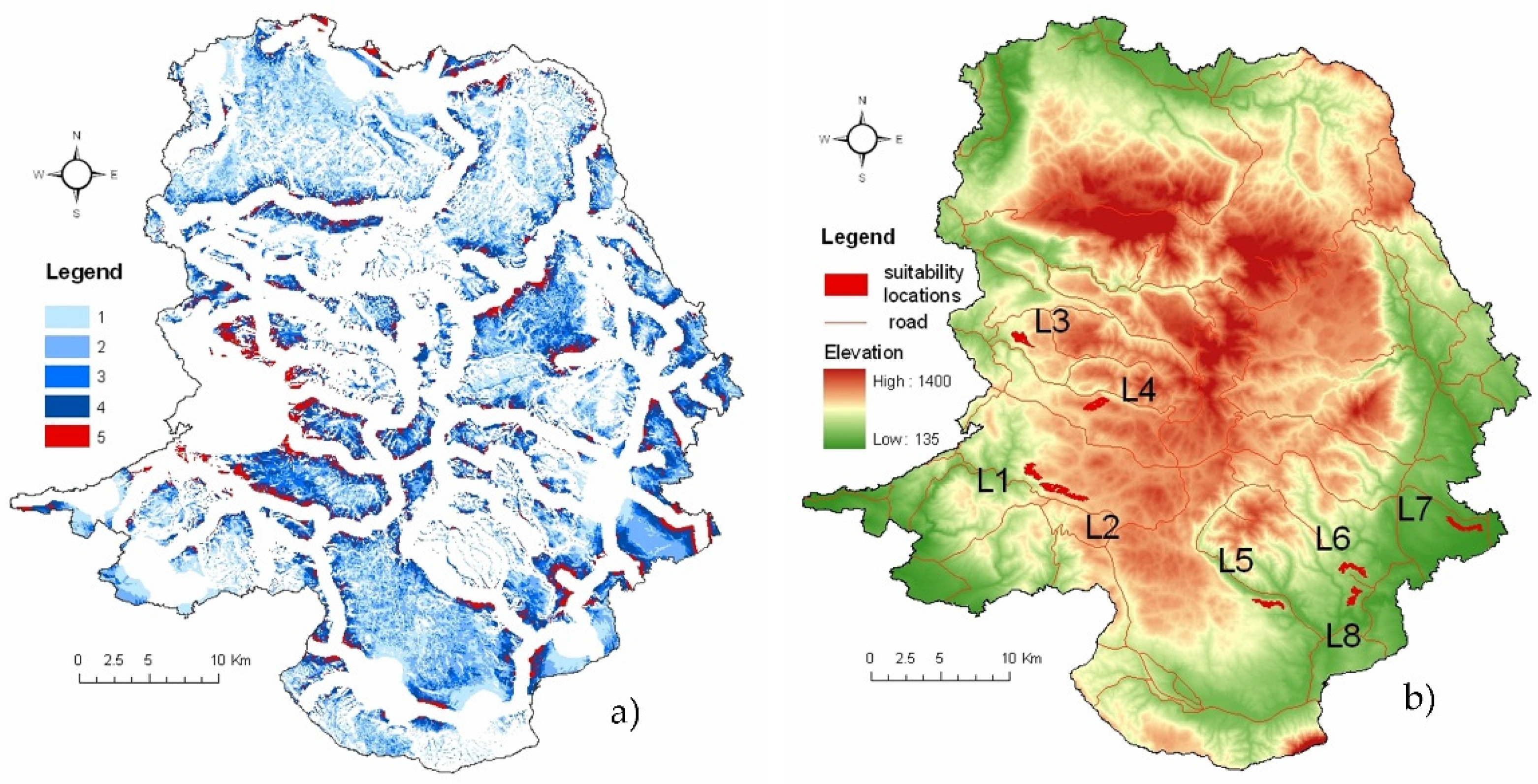
2.4.5. Extraction and Ranking of Suitable Locations

The extraction of suitable locations presents the extraction of cells with the highest x_i values from the final suitability map. They represent potentially the most suitable alternatives for the AD locations. The filtration of the most suitable alternatives (cells with the highest x_i) is conducted with the combined use of GIS arithmetic operations and inquiries. As a result, the suitable locations were obtained which are converted in the vector form meeting a certain level of suitability.

The final decision or recommendation should be based on the suitable locations’ ranking. The ranking is completed in order to assess every location with the established goals of the analysis. This model proposes the use of MAIRCA (MultiAttributive Ideal-Real Comparative Analysis) method for the selection of the most suitable location. MAIRCA was developed in 2014 by the Center for Logistics Research at the University of Defence in Belgrade [58].

The main assumption of MAIRCA method is in the determination of the gap between ideal and empirical weights. The summation of gaps for each criterion gives the total gap for every observed alternative. At the end, it comes to the alternatives ranking, where the best ranked alternative is the one with the smallest value for the total gap. The alternative with the smallest value for the total gap is the alternative which had values closest to the ideal weights according to the largest number of criteria (ideal criteria values). The MAIRCA method is conducted in six steps:

Step 1. The formation of the initial decision matrix (X). The criteria values (x_ij, i = 1, 2, ….n; j = 1, 2, …m) are determined in the initial decision Equation (22) for each of the observed alternatives.

$$X=\begin{array}{c}\\ A_1\\ A_2\\ \mathrm{...}\\ A_m\end{array}\begin{array}{c}\begin{array}{cccc}{C}_1& C_2& \mathrm{...}& C_n\end{array}\\ \left[\begin{array}{cccc}{x}_{11}& x_{12}& \mathrm{...}& x_{1n}\\ x_{21}& x_{22}& & x_{2n}\\ \mathrm{...}& \mathrm{...}& \mathrm{...}& \mathrm{...}\\ x_{m1}& x_{22}& \mathrm{...}& x_{mn}\end{array}\right]\end{array}$$

(22)

Equation (22) are obtained according to the personal preferences of the DM or by aggregation of experts’ decisions.

Step 2. Preference determination according to the alternative selection $P_{A_i}$. During alternative selection, the DM is neutral to the process. In fact, he does not have preference to any of the proposed alternatives. The main assumption is that DM does not take into account the probabilities of any alternative selection. The DM perceives the alternatives as if any of them can have equal probability of appearance, so the preference to choose one of them from m possible alternatives is:

$$P_{A_i}=\frac{1}{m};{\displaystyle \sum _{i=1}^m{P}_{A_i}}=1,i=1,2,\mathrm{...},m$$

(23)

where m denotes the total number of choices.

In the decision making analysis, with the given probabilities we assume that the DM is neutral towards the risk. In that case, all the preferences are equal according to the selection of certain alternatives

$$P_{A_1}=P_{A_2}=\mathrm{...}=P_{A_m}$$

(24)

where m denotes the total number of choices.

Step 3. The calculations of theoretical evaluation matrix elements ($T_p$). Theoretical evaluation matrix is created ($T_p$) with format n × m (n is the total criteria number, m is the total number of alternatives). Theoretical evaluation matrix elements ($t_{pij}$) are calculated as the multiplication of the preferences according to the alternatives $P_{A_i}$ and criteria weights ($w_i,i=1,2,\mathrm{...},n$)

$$T_p=\begin{array}{c}\\ \begin{array}{c}{P}_{A_1}\\ P_{A_2}\\ \mathrm{...}\\ P_{A_m}\end{array}\end{array}\begin{array}{c}\begin{array}{cccc}{w}_1& w_2& \mathrm{...}& w_n\end{array}\\ \left[\begin{array}{cccc}{t}_{p11}& t_{p12}& \mathrm{...}& t_{p1n}\\ t_{p21}& t_{p22}& & t_{p2n}\\ \mathrm{...}& \mathrm{...}& \mathrm{...}& \mathrm{...}\\ t_{pm1}& t_{pm2}& \mathrm{...}& t_{pmn}\end{array}\right]\end{array}=\begin{array}{c}\\ P_{A_1}\\ P_{A_2}\\ \mathrm{...}\\ P_{A_m}\end{array}\begin{array}{c}\begin{array}{cccc}{w}_1\hspace{1em}& w_2\hspace{1em}& \mathrm{...}& w_n\hspace{1em}\end{array}\\ \left[\begin{array}{cccc}{P}_{A_1}{w}_1& P_{A_1}{w}_2& \mathrm{...}& P_{A_1}{w}_n\\ P_{A_2}{w}_1& P_{A_2}{w}_2& & P_{A_2}{w}_n\\ \mathrm{...}& \mathrm{...}& \mathrm{...}& \mathrm{...}\\ P_{A_m}{w}_1& P_{A_m}{w}_2& \mathrm{...}& P_{A_m}{w}_n\end{array}\right]\end{array}$$

(25)

Because the DM is neutral to the initial selection of the alternatives, all preferences ($P_{A_i}$) are equal for all alternatives. Then, the Equation (25) can be shown in the Equation (26)

$$\begin{array}{ccc}& & \\ T_p& =& P_{A_i}\end{array}\begin{array}{c}\begin{array}{cccc}{w}_1& w_2& \mathrm{...}& w_n\end{array}\\ \left[\begin{array}{cccc}{t}_{p1}& t_{p2}& \mathrm{...}& t_{pn}\end{array}\right]\end{array}\begin{array}{cc}& \\ =& P_{A_i}\end{array}\begin{array}{cccc}{w}_1& w_2& \mathrm{...}& w_n\\ [P_{A_i}{w}_1& P_{A_i}{w}_2& \mathrm{...}& P_{A_i}{w}_n]\end{array}$$

(26)

where n is the total number of criteria, $t_{pi}$ is theoretical evaluation.

Step 4. Determination of real evaluation Equation (27).

$$T_r=\begin{array}{c}\\ A_1\\ A_2\\ \mathrm{...}\\ A_m\end{array}\begin{array}{c}\begin{array}{cccc}{C}_1& C_2& \mathrm{...}& C_n\end{array}\\ \left[\begin{array}{cccc}{t}_{r11}& t_{r12}& \mathrm{...}& t_{r1n}\\ t_{r21}& t_{r22}& & t_{r2n}\\ \mathrm{...}& \mathrm{...}& \mathrm{...}& \mathrm{...}\\ t_{rm1}& t_{rm2}& \mathrm{...}& t_{rmn}\end{array}\right]\end{array}$$

(27)

where n is the total number of criteria, m is the total number of alternatives.

The calculation of real evaluation matrix elements ($T_r$) is conducted by multiplying the real evaluation matrix elements ($T_p$) and elements of the initial decision making matrix ($X$) according to the equation:

(a)

For the “benefit” type criteria (the bigger criterion value is desirable)

$$t_{rij}=t_{pij}\left(\frac{x_{ij}-x_i^{-}}{x_i^{+}-x_i^{-}}\right)$$

(28)

(b)

For the “cost” type criteria (the smaller criterion value is desirable)

$$t_{rij}=t_{pij}\left(\frac{x_{ij}-x_i^{+}}{x_i^{-}-x_i^{+}}\right)$$

(29)

where $x_{ij}$, $x_i^{+}$ i $x_i^{-}$ denote elements of the initial decision making matrix ($X$), $x_i^{+}$ and $x_i^{-}$ are defined as:

• $x_i^{+}=\max \left(x_1,x_2,\mathrm{...},x_m\right)$ are the maximum values of the marked criterion by its alternatives.
• $x_i^{-}=\min \left(x_1,x_2,\mathrm{...},x_m\right)$ are the minimum values of the marked criterion by its alternatives.

Step 5. The calculation of the total gap matrix ($G$). The elements of the matrix $G$ are calculated as the difference (gap) between theoretical ($t_{pij}$) and real evaluations ($t_{rij}$), or by actually subtracting the elements of the theoretical evaluation matrix ($T_p$) with the elements of the real evaluation matrix ($T_r$).

$$G=T_p-T_r=\left[\begin{array}{cccc}{g}_{11}& g_{12}& \mathrm{...}& g_{1n}\\ g_{21}& g_{22}& \mathrm{...}& g_{2n}\\ \mathrm{...}& \mathrm{...}& \mathrm{...}& \mathrm{...}\\ g_{m1}& g_{m2}& \mathrm{...}& g_{mn}\end{array}\right]=\left[\begin{array}{cccc}{t}_{p11}-t_{r11}& t_{p12}-t_{r12}& \mathrm{...}& t_{p1n}-t_{r1n}\\ t_{p21}-t_{r21}& t_{p22}-t_{r22}& \mathrm{...}& t_{p2n}-t_{r2n}\\ \mathrm{...}& \mathrm{...}& \mathrm{...}& \mathrm{...}\\ t_{pm1}-t_{rm1}& t_{pm2}-t_{rm2}& \mathrm{...}& t_{pmn}-t_{rmn}\end{array}\right]$$

(30)

where n is the total number of criteria, m is the total number of alternatives.

Gap $g_{ij}$ takes values from the interval $g_{ij}\in \left[0,\left(t_{pij}-t_{rij}\right)\right]$, according to Equation (31)

$$g_{ij}=\{\begin{array}{ll}0,& if\hspace{1em}{t}_{pij}=t_{rij}\\ t_{pij}-t_{rij},& if\hspace{1em}{t}_{pij}>t_{rij}\end{array}$$

(31)

It is desirable that $g_{ij}$ goes to zero ($g_{ij}\to 0$) because the alternative with the smallest difference between the theoretical ($t_{pij}$) and real evaluation ($t_{rij}$) is chosen. If the alternative $A_i$ for the criterion $C_i$ has a theoretical evaluation value equal to the real evaluation value ($t_{pij}=t_{rij}$), then the gap for the alternative $A_i$ for the criterion $C_i$ is $g_{ij}=0$. In fact, the alternative $A_i$ for the criterion $C_i$ is the best (ideal) alternative ($A_i^{+}$).

If the alternative $A_i$ for the criterion. $C_i$ has a theoretical evaluation value. $t_{pij}$ and the real ponder value $t_{rij}=0$, than the gap for the alternative. $A_i$ for the criterion $C_i$ is $g_{ij}=t_{pij}$. In fact, the alternative $A_i$ is for the criterion $C_i$ the worst (anti-ideal) alternative ($A_i^{-}$).

Step 6. The calculation of the final values of the criteria functions ($Q_i$) for the alternatives. The values of the criteria functions are obtained from the sum of gaps ($g_{ij}$) for the alternatives, or just the sum of the matrix elements ($G$) in columns, using Equation (32)

$$Q_i={\displaystyle \sum _{j=1}^n{g}_{ij}},i=1,2,\mathrm{...},m$$

(32)

2.5. Sensitivity Analysis

The following step is to examine the solution stability (for the best alternatives) in the change of certain initial data. The purpose of this is to identify the change effects of entry data (geographic data and DM preferences) to exit data (the best alternative). It is reasonable that the most interesting aspect is examining the solution stability of the changes of relative weights, which are representative of subjectivity in the MCDA.

2.6. GIS Visualization of the Final Solutions and Recommendations

GIS visualization of the final solutions for the location selection according to the DM and interest groups is generally conducted through cartographic material, graphs, tables, etc. [31].

3. Results and Discussion

3.1. Studied Area

Regarding the geomorphological structure of the mountain systems in Serbia, the most suitable locations for the AD are situation at the Carpathians-Balkan mountain ranges. The Carpathians mountain massif is especially suitable due to its location, significance and karst geological structure meaning that the terrain fits well with the AD operational criteria. This massif is the biggest karst area in Serbia. The existence of a military range in this region also supports the suitability of establishing AD in this area.

The Carpathian area is located in the eastern part of Serbia and it is geographically set between 43°45′ and 44°15′ north latitude and between 21°26′ and 22°04′ east longitude. The territory has 1643 km². The whole area is defined by a plateau character with a complex tectonic and morphological structure along with distinctive small river valleys. This region is characterized by a greater number of forests. The dominant geological structure is karst. The additional benefit is the existence of local and regional roads and railroads which enables cheaper transport of heavy ammunition loads. (Figure 3).

3.2. Identification of Criteria that Influence the Selection of AD Location

According to the analysis of the environmental regulations, safety procedures when handling ammunition, public standards and a literature overview, nine restrictions are adopted in order to select a suitable AD location. These restrictions determine which areas should be ruled out from the analysis (

Table 1. Description of restrictions criteria.

Restriction	Description	Buffer Zones/Exclusion
R1	Protected areas. These are regarded as areas with highly prominent geological, biological, ecosystem and terrain diversity and according to the protection law are declared as protected areas of public interest [59].	<1000 m
R2	Urban areas. The social implications of the settlements that are near the AD locations are considered as a very important restriction due to safety issues. This influence should be assessed according to strict state regulations [39].	<2000 m
R3	Land use restrictions. Information about land use is a significant restriction. Among the numerous initiatives which provide land use information, the project CORINE is emphasized due to its methodology which allows providing sufficient and consistent information for Europe [60].	Artificial surfaces (all)
		Damp areas (all)
		Water surfaces (all) *
R4	Slope. Topography with steep slopes is generally considered as less suitable for AD location due to extra building and functioning costs [39].	>15%
R5	Distance from roads and railways. Although AD were built according to the safety and construction standards and have solid construction, practice suggests ensuring a safe distance from roads and railways [39].	<500 m
R6	Electric power line. Electric power lines are forbidden above and across AD sites due to the high risk of accidents [39].	<200 m
R7	The distance from important public objects. Industrial facilities must not be located near AD locations. Also, the presence of the AD can have a negative influence on tourism sites and areas [39].	<1000 m
R8	Minerals. It is required that potential locations for the AD do not have metal ores (manganese, iron, etc.) which affect the frequency and the intensity of lightning, so the AD safety would be in jeopardy [39].	Metal ores
R9	Military ranges. Military facilities are under the special safety status of the Ministry of Defence. Due to army units’ training and other military activities, it is necessary that AD are at a safe distance from such facilities [39].	<1000 m

*: The first level of CORINE hierarchy nomenclature.

).

Unlike the restrictions, which can be suitable or unsuitable, evaluation criteria are generally assessed on a continuous scale. Their purpose is to express the suitability of certain alternatives (cell)) [61].

Table 2. Description of evaluation criteria.

Evaluation Criteria	Description
C1	Distance from roads and railways. Ammunition transport is specific because it requires roads to the AD location along with the use of local roads and railways. So, the new roads should be as short as possible [39].
C2	Distance from urban areas. An AD location near urban areas can have negative influences on the people and the environment. It is required that AD are as far as possible from settlements [39].
C3	Land cover/use. The land use is considered as the environmental protection factor. Land use data were taken from the CORINE Land Cover 2006 (CLC2006) database. CORINE nomenclature has five main categories but three of them are excluded from the analysis. Evaluation criteria will deal with the third level of land use classification: Arable land (2.1.1.–2.1.3.), Permanent crops (2.2.1.–2.2.3.), Pastures 2.3.1., Heterogeneous agricultural areas 2.4.1.–2.4.4., Forests (Broad-leaved 3.1.1., Coniferous 3.1.2. and Mixed 3.1.3.), Scrub and/or herbaceous vegetation associations (3.2.1.–3.2.4.) and Open spaced with little or no vegetation (3.3.1.–3.3.4.). AD should be located at the areas where the impact on land use would be minimal. Coniferous forests should be avoided due to latent danger from fire. (3.1.2.) [60].
C4	Slope. AD should be sited at physically suitable locations. Areas with steep slopes are generally considered as less suitable or unsuitable due to extra expenses required for building and maintenance. It is recommended that chosen areas are as flat as possible [39].
C5	Distance from power lines. Due to the increased fire and explosion hazard, it is necessary that the AD is far from power lines [39].
C6	Distance from military ranges. The distance from the AD to military ranges should be short due to tactical, economic and time saving factors [39].

shows the adopted evaluation criteria.

The presented criteria and restrictions for the AD location are not final. They are adjusted according to the characteristics of the region and the military and state regulations in Serbia [38,39,59,62]. Other criteria and restrictions like distance to geological water courses or aquifers, areas which have a propensity to suffer earthquakes or high risk of floods are omitted from this study due to the compact karst nature of the Carpathian Mountains and their monolith pedological constituency so they would not have different spatial influences.

3.3. Data Gathering and Entry

Every criteria entered into GIS is presented in the form of spatial vector or rasterized maps, the layers of which present different alternatives with different intervals or scaled values. During data entry and the building of the spatial criteria and restrictions database, all GIS processes (digitalization, conversion, 3D analysis, etc.) are completed using integrated software tools in ArcGIS 10.2. The data sources and the design of GIS data sets are given in

Table 3. Data sources for input layers in land suitability assessment for the Carpathian region.

Layers		Data Source	Derived Map
Restrictions	Protected areas	Referral map no. 1, special area use [62].	Map of the protection buffers for the protected areas
	Urban areas	CORINE Land Cover 2006 (100 × 100) [60].	Map of the protection buffers for the urban areas
	Land cover/use		Map land use classes according to the CLC2006 nomenclature
	Slope	Digital terrain model (DMT 25) [63].	Map with slope values greater than 15°
	Roads	Digital topographic map (DTKP 300), 1:300,000 [64].	Map of the protection buffers for the roads
	Power lines		Map of the protection buffers for the power lines
	Military ranges		Map of the protection buffers for the military ranges and other facilities
	Important public objects	Referral map: Natural resources, environment protection, protection of the cultural and historical legacy, tourism [62].	Map of the protection buffers for the important industrial and tourist locations
	Metal ores	Mineral deposits and mining districts of Serbia Compilation map and GIS databases [65].	Map of the protection for the areas with metal ores
Evaluation criteria	Distance from urban areas	CORINE Land Cover 2006 (100 × 100) [60].	Distance map
	Land cover/use		Map land use classes according to the CLC2006 nomenclature
	Distance from roads and railway	Digital topographic map (DTKP 300), 1:300,000 [64].	Distance map
	Distance from power lines		Distance map
	Distance from the military ranges		Distance map
	Slope	Digital terrain model (DMT 25) [63].	Map with slopes between 0°and 15°

.

3.4. GIS-MCDA Evaluation

This phase consists of the aggregation of restrictions, standardization, weighting and sum analysis of all criteria considered in the decision making process. This is shown in Figure 4.

3.4.1. The Design and Aggregation of the Restriction Map

Aggregation of restrictions given in Table 1 gives “free” territory in the Carpathian region suitable for the AD location. Restrictions presented in the shape of thematic layers are created using Boolean (logical) algebra. Every restriction map is converted into a rasterized form and subsequently reclassified. Raster cell (alternatives) for the excluded area gets zero value while the others get a value of one. (Table 1). The total restriction map is created when all restriction layers are aggregated. Afterwards, the newly created raster cell layer (score 1) represents suitable AD locations (Figure 4).

The analysis of the thematic layer displayed in Figure 4 shows that 325 km² or 19.8% of all Carpathian region territory has no AD location limits. The relatively low suitability of this region for AD is the result of the huge diversity of the relief scarcity and rigid spatial and safety military required restrictions. This area consists of 519,245 cells (resolution 25 m × 25 m) denoting alternatives or the potential sites for the AD location which are the subject of the following suitability evaluation.

3.4.2. Individual Assessment of the Evaluation Criteria and Standardization

For further decision making analysis, detailed criteria maps are to be converted into joint intercomparable forms. Every criteria map is converted into raster and then reclassified according to the standardized class values from

Table 4. Evaluation criteria description and standardization.

Evaluation Criteria	Description	Intensity of importance
		1	2	3	4	5
		Very Low Suitability	Low Suitability	Moderate Suitability	High Suitability	Very High Suitability
C1	Distance from roads and railways	>1500 m	1250–1500 m	1000–1250 m	750–1000 m	500–750 m
C2	Distance from urban areas	1000–1250 m	1250–1500 m	1500–1750 m	1750–2000 m	>2000 m
C3 *	Land cover/use	(211–213; 312)	(241–244; 221–223)	(311; 313)	(321–324; 331–334)	(231)
C4 **	Slope	12°–15°	9°–12°	6°–9°	3°–6°	<3°
C5	Distance from power lines	>1400 m	1100–1400 m	800–1100 m	500–800 m	200–500 m
C6	Distance from military ranges	>5000 m	4000–5000 m	3000–4000 m	2000–3000 m	1000–2000 m

*: Level 3 of the CORINE nomenclature; **: Values are given for the mountain relief.

. Thus, every raster cell (alternative) is assigned a value on the shared scale from 1 to 5, where 1 denotes very low location suitability and 5 very high location suitability for the AD location. Obtained reclassified maps are thus converted into operational raster layers appropriate for the WLC. The alternative’s suitability in the criteria maps is usually symbolized with different color nuances so the lighter nuances correspond to the least suitable areas while darker ones represent the most suitable alternatives for the AD locations.

3.4.3. The Comparison and Relative Assessment of the Criteria Weights (DEMATEL-ANP)

Experts used the linguistic scale in order to evaluate criteria in the first step of the DEMATEL method application: 0—no influence; 1—low influence; 2—medium influence; 3—high influence; 4—very high influence. The results of the expert’s comparison in pairwise criteria are shown in

Table 5. Expert comparison matrix in the paired criteria.

DM1							DM6
Criteria	C1	C2	C3	C4	C5	C6	Criteria	C1	C2	C3	C4	C5	C6
C1	0	3	3	3	3	4	C1	0	2	2	3	2	4
C2	2	0	3	3	2	2	C2	2	0	2	3	3	3
C3	1	1	0	2	1	1	C3	1	2	0	2	2	1
C4	1	3	3	0	1	3	C4	2	3	2	0	0	1
C5	2	1	2	3	0	3	C5	2	2	2	3	0	2
C6	1	2	2	1	2	0	C6	1	2	2	2	1	0
DM2							DM7
Criteria	C1	C2	C3	C4	C5	C6	Criteria	C1	C2	C3	C4	C5	C6
C1	0	2	3	3	2	4	C1	0	2	3	2	2	3
C2	2	0	3	3	3	3	C2	2	0	3	3	2	0
C3	1	2	0	2	2	0	C3	2	3	0	2	3	2
C4	2	4	1	0	2	2	C4	1	4	2	0	2	1
C5	1	2	2	1	0	3	C5	2	1	2	2	0	3
C6	2	1	2	3	2	0	C6	2	1	1	1	2	0
DM3							DM8
Criteria	C1	C2	C3	C4	C5	C6	Criteria	C1	C2	C3	C4	C5	C6
C1	0	3	2	2	3	4	C1	0	1	2	3	2	3
C2	2	0	2	3	3	0	C2	2	0	3	3	2	2
C3	1	3	0	1	2	1	C3	1	2	0	2	2	2
C4	2	3	2	0	2	1	C4	2	4	1	0	1	2
C5	1	2	2	2	0	4	C5	1	2	2	1	0	3
C6	1	2	1	1	2	0	C6	3	1	2	1	1	0
DM4							DM9
Criteria	C1	C2	C3	C4	C5	C6	Criteria	C1	C2	C3	C4	C5	C6
C1	0	2	2	3	3	3	C1	0	1	2	3	2	4
C2	1	0	3	3	3	3	C2	3	0	3	3	3	2
C3	1	2	0	0	2	2	C3	2	3	0	2	2	2
C4	1	3	2	0	2	2	C4	2	4	2	0	3	2
C5	2	2	1	3	0	3	C5	2	2	2	0	0	3
C6	2	1	2	2	2	0	C6	2	1	1	1	2	0
DM5							DM10
Criteria	C1	C2	C3	C4	C5	C6	Criteria	C1	C2	C3	C4	C5	C6
C1	0	2	2	0	2	3	C1	0	2	3	2	2	3
C2	2	0	2	3	2	2	C2	2	0	2	3	3	0
C3	1	2	0	2	2	1	C3	1	2	0	2	2	2
C4	2	3	1	0	3	2	C4	2	3	2	0	2	3
C5	2	1	2	2	0	3	C5	2	2	1	1	0	3
C6	2	1	2	2	2	0	C6	2	1	1	2	2	0

.

Aggregation of experts’ decisions is completed according to Equation (1) and the average matrix Z is obtained as it is shown in

Table 6. The average matrix Z.

Criteria	C1	C2	C3	C4	C5	C6
C1	0	2	2.2727	2.2727	2.2727	3.4545
C2	1.90909	0	2.5454	3	2.5454	1.7272
C3	1.1818	2.1818	0	1.72727	2	1.3636
C4	1.72727	3.3636	1.72727	0	1.8181	1.909
C5	1.72727	1.6363	1.8181	1.8181	0	2.909
C6	1.72727	1.2727	1.6363	1.6363	1.909	0

.

Equations (3) and (4) are used to normalize elements from matrix Z so the initial direct-relation matrix D is obtained, Equation (2), shown in

Table 7. The normalized initial direct-relation matrix D.

Criteria	C1	C2	C3	C4	C5	C6
C1	0	0.176	0.2	0.2	0.2	0.304
C2	0.168	0	0.224	0.264	0.224	0.152
C3	0.104	0.192	0	0.152	0.176	0.12
C4	0.152	0.296	0.152	0	0.16	0.168
C5	0.152	0.144	0.16	0.16	0	0.256
C6	0.152	0.112	0.144	0.144	0.168	0

.

Equations (5)–(7) are used to determine the elements of the total relation criteria matrix (T) (

Table 8. The total relation matrix T.

Criteria	C1	C2	C3	C4	C5	C6
C1	1.1983	1.6022	1.5638	1.6194	1.6335	1.7897
C2	1.3147	1.4312	1.5522	1.6366	1.6189	1.6449
C3	0.9837	1.2421	1.0379	1.2130	1.2383	1.2532
C4	1.2195	1.5575	1.4040	1.3262	1.4714	1.5434
C5	1.1290	1.3342	1.3001	1.3464	1.2203	1.4966
C6	0.9883	1.1431	1.1256	1.1653	1.1928	1.1104

). Matrix T elements are used in the following step to calculate the cause and effect relationship diagram (CERD).

Equations (9) and (10) sum the matrix T values in rows (D_i) and columns (R_i). The summed values of the matrix T in rows and columns are shown in

Table 9. The sums of matrix T values for six criteria.

Criteria	C1	C2	C3	C4	C5	C6	Di	Ri	D + R	D − R
C1	1.1983	1.6022 *	1.5638 *	1.6194 *	1.6335 *	1.7897 *	9.4068	6.8335	16.2403	2.5733
C2	1.3147	1.4312 *	1.5522 *	1.6366 *	1.6189 *	1.6449 *	9.1985	8.3103	17.5087	0.8882
C3	0.9837	1.2421	1.0379	1.213	1.2383	1.2532	6.9683	7.9836	14.9519	−1.0153
C4	1.2195	1.5575 *	1.4040 *	1.3262	1.4714 *	1.5434 *	8.5219	8.3069	16.8288	0.2151
C5	1.129	1.3342	1.3001	1.3464	1.2203	1.4966 *	7.8266	8.3752	16.2018	−0.5486
C6	0.9883	1.1431	1.1256	1.1653	1.1928	1.1104	6.7255	8.8382	15.5637	−2.1127

* Values greater than the threshold value.

.

The threshold value was derived from the average of elements in matrix T, which was calculated by using Equation (11). According to the results shown in Table 4 and Table 5 and Equation (11), CERD is designed (Figure 5) showing the criteria interrelationship. The values of t_ij in Table 5, which are greater than α (1.351), are shown as t_ij*, which present the interaction between perspectives. As an example, t₁₂ (1.6022) > α (1.351); hence, the arrow in the cause and effect diagram was drawn from C₁ to C₂.

The DEMATEL method gave CERD as the result of the data processing which serves as the basis for the ANP method utilization and better understanding relationship network between the criteria. Interrelationships between the criteria are defined according to the calculations in the matrix T, threshold value α and CERD. The understanding of the network considerably simplifies the understanding of the ANP method modeling used to calculate relative criteria weights.

The first step of the ANP method incorporates the total-influence matrix T into ANP model and, using Equations (13)–(18), the unweighted supermatrix is obtained (

Table 10. Unweighted supermatrix.

Criteria	C1	C2	C3	C4	C5	C6
C1	0.23	0.37	0.35	0.37	0.35	0.35
C2	0.50	0.37	0.653	0.51	0.51	0.51
C3	0.50	0.62	0.35	0.49	0.49	0.49
C4	0.31	0.35	0.35	0.26	0.35	0.33
C5	0.36	0.34	0.35	0.41	0.27	0.41
C6	0.33	0.31	0.31	0.33	0.37	0.26

).

In the following step, the elements of the weighted Equation (21) are calculated using Equations (19) and (20). Elements of the weighted supermatrix are shown in

Table 11. Weighted supermatrix.

Criteria	C1	C2	C3	C4	C5	C6
C1	0.06	0.07	0.07	0.09	0.09	0.08
C2	0.10	0.08	0.145	0.10	0.10	0.10
C3	0.10	0.14	0.08	0.10	0.10	0.10
C4	0.07	0.09	0.09	0.07	0.09	0.08
C5	0.09	0.09	0.09	0.10	0.07	0.10
C6	0.08	0.08	0.08	0.09	0.09	0.07

.

The elements of the limited supermatrix are calculated in the last step of the ANP method, the vectors of which present the weighted coefficients of the model (

Table 12. Weighted coefficients of the criteria.

Criteria	Weighted Coefficient	Rank
Distance from the roads and railways (C1)	0.182	3
Distance from urban areas (C2)	0.211	1
Land cover/use (C3)	0.204	2
Slope (C4)	0.172	4
Distance from power lines (C5)	0.097	6
Distance from the military ranges (C6)	0.134	5

).

3.4.4. Aggregation Results (Suitability Map)

The WLC method is used to sum standardized criteria values, according to Equation (21). The criteria weights, obtained from the DANP method, are multiplied with the raster cell score of each criterion creating the final suitability map (Figure 6a).

The final suitability map is presented in the same value interval as for each criterion, from 1 to 5. The higher cell values indicate areas more suitable for the AD location.

3.4.5. Extraction and Ranking of Suitable Locations

The final step of the analysis is the selection of cells with the highest values from the final suitability map. These are cells with pixels that have a value of 5. As the final result of the used model, 5803 potentially suitable locations (alternatives) for the AD are identified in the Carpathian region. Those are mainly locations with very small areas of between 400 and 1 km². The total area of the suitable locations is 44.5 km² (Figure 6a).

Taking into account that the optimum area for the AD location is a minimum of 0.5 km², according to the explosive safety rules for the medium sized AD [39,40,41], GIS-SQL operation has extracted areas larger than 0.5 km². Eight acceptable locations are identified in the Carpathian region after the analysis is conducted (Figure 6b).

The ranking of the suitable locations is completed after the identification, so the most suitable location is determined using the MAIRCA method. First of all, the initial decision matrix is designed (

Table 13. Initial matrix for the sustainable locations evaluation.

Location Designation	C1	C2	C3	C4	C5	C6
L 1	3.828	5.000	3.720	2.723	1.000	4.255
L 2	4.675	5.000	3.000	3.452	1.000	2.587
L 3	4.515	4.836	3.289	3.491	1.000	4.069
L 4	4.421	5.000	3.555	2.839	1.000	4.397
L 5	4.717	5.000	3.430	4.401	1.000	1.000
L 6	4.695	5.000	3.925	3.847	1.000	1.000
L 7	4.688	5.000	2.000	4.99	1.000	1.000
L 8	4.688	5.000	3.971	4.001	1.000	1.000

), and, afterwards, the criteria normalization is completed using Equations (26) and (27). Data shown in Table 13 represent average values of the location suitability obtained using GIS Zonal statistical operation from the reclassified evaluation criteria maps.

Because all alternatives are equal and have a value of 1 for the criterion C5, it can be eliminated. It has no influence on the location ranking. Weight criteria is evenly distributed from C5 to other criteria by adding Δw_C5 = w_C5/5 = 0.097/5 = 0.0194 to each of them.

After the formation of the initial matrix (Table 13), preferences according to the alternative is calculated using Equation (23).

$$P_{A_i}=\frac{1}{m}=\frac{1}{8}=0.125$$

(33)

where m denotes the number of alternatives. In that case, all preferences are equal and are presented as follows,

$$P_{A_1}=P_{A_2}=\mathrm{...}=P_{A_8}=0.125$$

(34)

The calculation T_p matrix elements (

Table 14. Matrix of the calculated theoretical evaluation T_p.

Location Designation	C1	C2	C3	C4	C6
L 1	0.0252	0.0288	0.0279	0.0239	0.0192
L 2	0.0252	0.0288	0.0279	0.0239	0.0192
L 3	0.0252	0.0288	0.0279	0.0239	0.0192
L 4	0.0252	0.0288	0.0279	0.0239	0.0192
L 5	0.0252	0.0288	0.0279	0.0239	0.0192
L 6	0.0252	0.0288	0.0279	0.0239	0.0192
L 7	0.0252	0.0288	0.0279	0.0239	0.0192
L 8	0.0252	0.0288	0.0279	0.0239	0.0192

) is conducted according to Equation (25),

$$t_{p32}=P_{A_3}\cdot w_2=0.125\cdot 0.230=0.0288$$

(35)

After the calculation of T_p, the next step calculates the matrix elements of the real evaluation T_r. These elements (

Table 15. Matrix of the calculated real evaluation T_p.

Location Designation	C1	C2	C3	C4	C6
L 1	0.0252	0.0288	0.0036	0.0239	0.0008
L 2	0.0012	0.0288	0.0138	0.0162	0.0102
L 3	0.0057	0.0000	0.0097	0.0158	0.0019
L 4	0.0084	0.0288	0.0059	0.0227	0.0000
L 5	0.0000	0.0288	0.0077	0.0062	0.0192
L 6	0.0006	0.0288	0.0007	0.0121	0.0192
L 7	0.0008	0.0288	0.0279	0.0000	0.0192
L 8	0.0008	0.0288	0.0000	0.0104	0.0192

) are obtained by multiplying matrix T_p with normalized elements of the initial matrix (Table 13). Elements’ normalization is completed by using Equation (28) (for C2) and Equation (29) (for C1, C3, C4 and C6). The real evaluation matrix element at the position t_r32 is obtained using Equation (28).

$$t_{r32}=t_{pij}\cdot \left(\frac{x_{ij}-x_i^{-}}{x_i^{+}-x_i^{-}}\right)=0.0288\left(\frac{4.836-4.836}{5.00-4.836}\right)=0.00$$

(36)

The total gap matrix elements are calculated using Equation (30) and they are shown in

Table 16. The total gap matrix.

Location Designation	C1	C2	C3	C4	C6
L 1	0.0000	0.0000	0.0244	0.0000	0.0184
L 2	0.0240	0.0000	0.0142	0.0077	0.0090
L 3	0.0195	0.0288	0.0183	0.0081	0.0173
L 4	0.0168	0.0000	0.0220	0.0012	0.0192
L 5	0.0252	0.0000	0.0203	0.0177	0.0000
L 6	0.0246	0.0000	0.0273	0.0119	0.0000
L 7	0.0244	0.0000	0.0000	0.0239	0.0000
L 8	0.0244	0.0000	0.0279	0.0135	0.0000

. The total gap matrix element at the position g₃₂ is obtained using Equations (30) and (31).

$$g_{22}=t_{p32}-t_{r32}=0.288-0.00=0.288$$

(37)

It is desirable that $g_{ij}$ has values that are close to zero ($g_{ij}\to 0$), because the alternative with the smallest difference between the ($t_{pij}$) and real evaluation ($t_{rij}$) is to be chosen.

The best ranking alternative, the one with the lowest gap value, is the location—L 1, as it is shown in

Table 17. Alternative ranking according to MAIRCA.

Alternative	Q	Rank
L 1	0.0427	1
L 2	0.0548	3
L 3	0.0919	8
L 4	0.0592	4
L 5	0.0631	5
L 6	0.0637	6
L 7	0.0483	2
L 8	0.0658	7

.

The best ranking alternative, the one with the lowest gap value, is the location—L 1.

3.5. Sensitivity Analysis

Sensitivity analysis is recommended in most of the MCDA processes as an instrument for testing the results’ stability against the subjectivity of the DM [66]. Sensitivity analysis is completed by changing the initial criteria weights [32], as it is shown in

Table 18. Combination of weights for the sensitivity analysis.

Scenarios	Criteria Weights
	C1	C2	C3	C4	C6
A—Equalized criteria weights	0.2000	0.2000	0.2000	0.2000	0.2000
B—Distance from the roads and settlements priority	0.3000	0.3000	0.1333	0.1333	0.1333
C−Land cover/use priority	0.1625	0.1625	0.3500	0.1625	0.1625
D−Slope priority	0.1625	0.1625	0.1625	0.3500	0.1625
E—Distance from the power lines and military ranges priority	0.1625	0.1625	0.1625	0.1625	0.3500

.

According to the recommendations [32], the sensitivity analysis of the location rankings has been conducted through five scenarios. The first scenario (A) deals with the equalized criteria weights w_i = 1/5 = 0.2000. The second scenario (B) favours criteria C₁ and C₂, w₁ = w₂ = 0.3000, while other criteria weights were evenly distributed, w₃ = w₄ = w₆ = 0.1333. The remaining three scenarios (C, D and E) favours one of the criteria, C₃, C₄ and C_6, respectively. The favoured criteria has a weight w = 0.3500, while the others have a value of 0.1625.

The resulting rankings are given in

Table 19. Alternative rankings for different scenarios.

Alternative	Alternative Ranks
	A	B	C	D	E
L 1	1	1	3	1	6
L 2	3	4	2	3	5
L 3	8	8	8	8	8
L 4	6	3	5	2	7
L 5	5	6	4	7	3
L 6	4	5	6	4	2
L 7	2	2	1	5	1
L 8	7	7	7	6	4

. Results show that assigning different weights (priorities) to the criteria leads to different rankings, i.e., the model is sensitive to these weights.

Comparing the first ranked alternatives in all scenarios, it can be concluded that the alternative L1 remained first in three out of five scenarios. In scenario C, the alternative L1 is in third place and in scenario E, it is in sixth place. Thus, the alternative L1 is superior to the others and the ranking presented in Table 17 is acceptable.

MAIRCA presents a new MCDA method so it should be compared with other already proven methods. There are different studies associated with location selection decisions that have been commonly carried out by using multi-criteria decision-making techniques, location problems with MOORA and COPRAS method [67,68,69], selecting distribution centers for a firm and location choice of distribution centers with VIKOR [70], location selection of logistics centres based on Fuzzy AHP and TOPSIS [71], and selection of logistics centres’ locations with fuzzy TOPSIS based on entropy weight [72]. The methods VIKOR, TOPSIS, MOORA and COPRAS are proposed in the previously stated references as prominent for location ranking. The above mentioned methods are compared with the MAIRCA method in order to compare location ranking.

Table 20. Alternative ranking using the methods VIKOR, TOPSIS, MOORA i COPRAS.

Alternative	VIKOR		TOPSIS		MOORA		COPRAS
	F	Rank	F	Rank	F	Rank	F	Rank
L 1	0.0863	1	0.3706	6	−0.1942	6	84.07	6
L 2	0.2561	4	0.5391	5	−0.1720	4	90.73	5
L 3	1.0000	8	0.3191	8	−0.2079	8	81.21	8
L 4	0.2512	3	0.3487	7	−0.2045	7	81.83	7
L 5	0.4271	5	0.5884	2	−0.1693	2	92.80	2
L 6	0.5129	6	0.5728	3	−0.1705	3	92.47	3
L 7	0.1702	2	0.6499	1	−0.1463	1	100.00	1
L 8	0.5686	7	0.5602	4	−0.1742	5	91.44	4

shows the results of alternatives’ ranking according to criteria from Table 13 using the methods VIKOR, TOPSIS, MOORA i COPRAS.

Comparing results obtained using the MAIRCA method (Table 17) with the results obtained from the methods VIKOR, TOPSIS, MOORA and COPRAS (Table 20), it can be seen that the alternative ranking for MAIRCA and VIKOR is similar. They are favoring alternatives L 1 and L 7. On the other hand, other methods suggest quite different rankings favoring alternatives L 7 and L 5.

MAIRCA and VIKOR are similar due to the same method of data normalization, defined by the Equations (28) and (29). In contrast, MOORA and TOPSIS use vector normalization, given in the Equation (38).

$$r_{ij}=\frac{x_{ij}}{\sqrt{{\displaystyle \sum _{i=1}^m{x}_{ij}^2}}}$$

(38)

where r_ij denotes normalized elements of the matrix, x_ij presents the elements of the initial matrix and m is the total number of alternatives. The COPRAS method uses simple normalization, benefit type, Equation (39),

$$r_{ij}=\frac{x_{ij}}{x_{ij}^{+}}$$

(39)

For the cost type criteria, Equation (40),

$$r_{ij}=\frac{x_{ij}}{x_{ij}^{-}}$$

(40)

where x_ij presents the elements of the initial matrix, and x⁻_ij and x⁺_ij are the minimum/maximum criteria values.

In order to compare alternatives with different methods in an adequate manner, linear normalization of initial data is used for all methods, keeping the original mathematic calculations. Obtained data are presented in

Table 21. Alternative ranking (VIKOR, TOPSIS, MOORA and COPRAS)—with linear normalization.

Alternative	VIKOR		TOPSIS		MOORA		COPRAS
	F	Rank	F	Rank	F	Rank	F	Rank
L 1	0.0863	1	0.5973	1	−0.1115	1	100.00	1
L 2	0.2561	4	0.5518	3	−0.2080	3	84.04	3
L 3	1.0000	8	0.3085	8	−0.5052	8	49.09	8
L 4	0.2512	3	0.5304	4	−0.2434	4	79.82	4
L 5	0.4271	5	0.4940	5	−0.2748	5	76.57	5
L 6	0.5129	6	0.4873	6	−0.2791	6	76.15	6
L 7	0.1702	2	0.5657	2	−0.1558	2	91.68	2
L 8	0.5686	7	0.4783	7	−0.2957	7	74.61	7

.

It can be concluded from Table 21 that the rankings for methods TOPSIS, COPRAS and MOORA are the same like for the MAIRCA, while it is slightly different for the VIKOR method. The alternative L1 is ranked first in all methods so it can be concluded that this alternative is superior and the ranking suggested in Table 17 is confirmed and found to be credible.

4. Conclusions

The selection of the optimum AD location using MCDA in GIS was for the first time conducted in this research for the Carpathian region in the Republic of Serbia. It represents a model that can be used in other areas with similar natural characteristics.

Multi-criteria techniques DEMATEL, ANP (DANP) and WLC inside GIS software are suggested in order to select suitable areas for AD locations. DANP is used for criteria weighting, and WLC is used for the weighting sums and final identification of suitable AD locations. The use of these methods is enabled by the ArcGis software solution ArcGIS Advanced 10.2, from ESRI. The implementation of the GIS-MCDA model was proven successful and justified, because, on the basis of nine restrictions and six evaluation criteria, suitable sites for the AD installation could be determined.

The model has identified a total 44.5 km² of the concerned region as the most suitable area for the AD location. Finally, eight suitable locations were found by restraining areas smaller than 0.5 km². The MAIRCA method found location L1 to be the most appropriate.

This model expands the frame of knowledge for FLP. The existing problem is considered using a new methodology, thus creating the basis for further theoretical and practical advancement. Moreover, the methodology used in this study highlights new criteria never considered before, but that were found to be crucial for the given area of research.

This procedure allows for the inclusion of other criteria, which are not considered here, such as distance to watercourses and streams, distance to geological water courses or aquifers, distance to protected areas, areas which have a propensity to suffer from earthquakes or at high risk of floods. These criteria and restrictions are not set out by military and state regulations. For example, slope is a crucial restriction here but elsewhere it could be treated differently. The addition or omission of certain restrictions and criteria can be designated in new regulations, rules and guidelines because, currently, Serbian law does not fully recognize criteria restrictions for hazardous material issues. All of these combined factors are important in the selection of suitable locations.

It should be mentioned that this study is not intended as an exhaustive overview but is intended to point future research in the right direction. Nevertheless, this study includes experts’ opinions and gives recommendations which are certainly valuable for future research in this area.

References

1. Bell, J.E. A simulated annealing approach for the composite facility location and resource allocation problem: A study of strategic positioning of US air force munitions. Ph.D. Thesis, Auburn University, Auburn, AL, USA, 2003. [Google Scholar]
2. Recknor, W.A.; Osborne, G.J. Pacific Air Forces, Munitions Divisions Chief; Air Force Logistics Management Agency: Montgomery, AL, USA, 1998.
3. Underwood, D.; Bell, J.E. Munitions Availability and the EAF. Air Force J. Logist. 1999, 23, 38–40. [Google Scholar]
4. Johnstone, D.P. Modelling the Pre-Positioning of Air Force Precision Guided Munitions. Master’s Thesis, Air Force Institute of Technology, Wright-Patterson Air Force Base, Montgomery County, OH, USA, 2002. [Google Scholar]
5. Ding, Y.J.; Wei, Q.; Hou, P.K.; Yuan, T. Fuzzy Synthetic Evaluation of the Ground to Air Missile Position Selection. Fire Control Command Control 2007, 4. [Google Scholar] [CrossRef]
6. Zhu, C.Z.; Gao, J.Z.; Zhang, P.; Cai, W.M. Position Selection of Ground-to-air Missile based on Fuzzy Synthetical Evaluation. Fire Control Command Control 2007, 1, 31–47. [Google Scholar]
7. Zhu, Y.; Shu, J.S. AHP for Selecting Missile Launch Position. Fire Control Command Control. 2002, 2, 19–35. [Google Scholar]
8. Zhang, T.W.; Yuan, S.Z. Study on Position Selection for Air Defense Group Based on Improved AHP and Set Pair Analysis. Command Control Simulation. 2008, 3. [Google Scholar] [CrossRef]
9. An, Q.J.; Li, Y.; An, J. Optimum Select of Ground to Air Missile Position Based on Consistent Triangular Fuzzy Number Complementary Judgment Matrix. Ordnance Ind. Autom. 2006, 8, 42–50. [Google Scholar]
10. Discussing the Issue of Surplus Weapons: Unplanned Explosions in Warehouses Ammunition in Southeast Europe. Available online: http://www.smallarmssurvey.org/fileadmin/docs/H-Research_Notes/SAS-Research-Note-41-BCMS.pdf (accessed on 20 December 2015).
11. Lazarević, J. Costs and Consequences: Unplanned Explosions and Demilitarization in South-east Europe. Special RASR Report; Small Arms Survey: Geneva, Switzerland, 2012. [Google Scholar]
12. Malczewski, J. Review article GIS-based multi-criteria decision analysis: A survey of the literature. Int. J. Geograp. Inform. Sci. 2006, 20, 703–726. [Google Scholar] [CrossRef]
13. Güzel, D.; Erdal, H. A Comparative Assessment of Facility Location Problem via fuzzy TOPSIS and fuzzy VIKOR: A Case Study on Security Services. Int. J. Bus. Soc. Res. 2015, 5, 49–61. [Google Scholar]
14. Zhang, X.; Wang, Z.; Lin, J. GIS Based Measurement and Regulatory Zoning of Urban Ecological Vulnerability. Sustainability 2015, 7, 9924–9942. [Google Scholar] [CrossRef]
15. Uribe, D.; Geneletti, D.; Castillo, R.F.; Orsi, F. Integrating Stakeholder Preferences and GIS-Based Multicriteria Analysis to Identify Forest Landscape Restoration Priorities. Sustainability 2014, 6, 935–951. [Google Scholar] [CrossRef]
16. Cagrici, H. Determining the Optimal Locations of Munitions’ Warehouse of the Multiple Launch Rocket Systems with Genetic Algorithms. Master’s Thesis, Turkish Army Military Academy, Ankara, Turkey, 2007. [Google Scholar]
17. Erdal, H. Optimization of Ammunition Distribution Network. Master’s Thesis, Turkish Army Military Academy, Ankara, Turkey, 2013. [Google Scholar]
18. Onan, K.; Ülengin, F.; Sennaroğlu, B. An evolutionary multi-objective optimization approach to disaster waste management: A case study of Istanbul, Turkey. Expert Syst. Appl. 2015, 42, 8850–8857. [Google Scholar] [CrossRef]
19. Di Matteo, U.; Pezzimenti, P.M.; Garcia, D.A. Methodological Proposal for Optimal Location of Emergency Operation Centers through Multi-Criteria Approach. Sustainability 2016, 8. [Google Scholar] [CrossRef]
20. Erden, T.; Coşkun, M.Z. Multi-criteria site selection for fire services: The interaction with analytic hierarchy process and geographic information systems. Nat. Hazards Earth Syst. Sci. 2010, 10, 2127–2134. [Google Scholar] [CrossRef]
21. Abdullahi, S.; bin Mahmud, A.R.; Biswajeet, P. Biswajeet, Spatial modelling of site suitability assessment for hospitals using geographical information system-based multicriteria approach at Qazvin city, Iran. Geocarto Int. 2014, 29, 164–184. [Google Scholar] [CrossRef]
22. Arabsheibani, R.; Kanani Sadat, Y.; Abedini, A. Land Suitability Assessment for Locating Industrial Parks: A Hybrid Multi Criteria Decision-Making Approach Using Geographical Information System. Geogr. Res. 2016. [Google Scholar] [CrossRef]
23. Tahcry, M.; Abbaspour, R.A.; Alavipanah, S.K. Multi criteria decision making based on DEMATEL and ANP techniques to select the optimum location for cemeteries, Isfahan City, Iran. J. Environ. Stud. 2014, 40, 463–480. [Google Scholar]
24. Safari, M.; Kakaei, R.; Ataei, M.; Karamoozian, M. Using fuzzy TOPSIS method for mineral processing plant site selection. Case study: Sangan iron ore mine (phase 2). Arab. J. Geosci. 2012, 5, 1011–1019. [Google Scholar] [CrossRef]
25. Sánchez-Lozano, J.M.; Teruel-Solano, J.; Soto-Elvira, P.L.; García-Cascales, M.S. Geographical information systems (GIS) and multi-criteria decision making (MCDM) methods for the evaluation of solar farms locations: case study in south-eastern Spain. Renew. Sustain. Energy Rev. 2013, 24, 544–556. [Google Scholar] [CrossRef]
26. Marinoni, O. A discussion on the computational limitations of outranking methods for land-use suitability assessment. Int. J. Geogr. Inf. Sci. 2006, 20, 69–87. [Google Scholar] [CrossRef]
27. Esmaelian, M.; Tavana, M.; Arteaga, F.J.S.; Mohammadi, S. A multicriteria spatial decision support system for solving emergency service station location problems. Int. J. Geogr. Inf. Sci. 2015, 29, 1187–1213. [Google Scholar] [CrossRef]
28. Farahani, R.Z.; Steadie, S.M.; Asgari, N. Multiple criteria facility location problems: A survey. Appl. Math. Model. 2010, 34, 1689–1709. [Google Scholar] [CrossRef]
29. Pourkhabbaz, H.; Javanmardi, S.; Sabokbar, H.F. Suitability Analysis for Determining Potential Agricultural Land Use by the Multi-Criteria Decision Making Models SAW and VIKOR-AHP (Case study: Takestan-Qazvin Plain). J. Agric. Sci. Technol. 2014, 16, 1005–1016. [Google Scholar]
30. Geneletti, D.; Beinat, E.; Chung, C.J.; Fabbri, A.G.; Scholten, H.J. Accounting for uncertainty factors in biodiversity impact assessment: lessons from a case study. Environ. Impact Assess. Rev. 2003, 23, 471–487. [Google Scholar] [CrossRef]
31. Malczewski, J. GIS and Multi-Criteria Decision Analysis; John Wiley and Sons: New York, NY, USA, 1999. [Google Scholar]
32. Pamučar, D.; Ćirović, G. The selection of transport and handling resources in logistics centres using Multi-Attributive Border Approximation area Comparison (MABAC). Expert Syst. Appl. 2015, 42, 3016–3028. [Google Scholar]
33. Eastman, J.R.; Kyen, P.A.K.; Toledano, J. A Procedure for Multiple-Objective Decision Making in GIS Under Conditions of Conflicting Objectives. In Proceedings of the Fourth European Conference on GIS (ESIG’93), Genova, Italy, 29 March–1 April 1993; Hents, J., Ottens, H.F.L., Scholten, H.J., Eds.; Volume 1, pp. 438–447.
34. Chang, N.B.; Parvathinathan, G.; Breeden, J.B. Combining GIS with fuzzy multi-criteria decision-making for landfill siting in a fast-growing urban region. J. Environ. Manag. 2008, 87, 139–153. [Google Scholar] [CrossRef] [PubMed]
35. Ehler, G.; Cowen, D.; Mackey, H. Design and Implementation of a Spatial Decision Support System for Site Selection. In Proceedings of the ESRI International User Conference, Palm Springs, CA, USA, 22–26 May 1995; p. 100.
36. Ma, Y.; Chen, L.; Lu, Y.; Yang, X. Research on Network Location Problem of Equipment Support Force Spatial Configuration. In Proceedings of the 2012 International IEEE Conference on Industrial Control and Electronics Engineering (ICICEE), Xi’an, China, 23–25 August 2012; pp. 388–391.
37. Cai, Y.X.; Yu, H.M.; Sun, Y.; Lu, S.J. Assistance Decision Model for Selecting the Disposition Regions of Ammunition Sites. J. Ordnance Eng. College. 2005, 1, 54–57. [Google Scholar]
38. SOG. Explosive material, flammable liquids and gases Law. Available online: http://www.paragraf.rs/propisi/zakon_o_eksplozivnim_materijama_zapaljivim_tecnostima_i_gasovima.html (accessed on 14 April 2016). (In Serbian)
39. Technical Management of the Serbian Army. Handbook for the Service of the Ammunition Depots (in Serbian); Technical Management of the Serbian Army: Belgrade, Serbia, 2002. [Google Scholar]
40. AASTP. Allied Ammunition Storage and Transport Publication (AASTP-1); North Atlantic Treaty Organization, Military Agency for Standardization: Brussels, Belgium, 2006; Volume 1. [Google Scholar]
41. United States Department of the Army. DAPAM 385-65. Explosive and Chemical Site Plan Development and Submission; United States Department of the Army: Washington, DC, USA, 2008.
42. Chang, K.T. Introduction to Geographic Information System; Tata McGraw Hill: New Delhi, India, 2006. [Google Scholar]
43. Wu, W.W.; Lee, Y.T. Developing global managers competencies using the fuzzy DEMATEL method. Expert Syst. Appl. 2007, 32, 499–507. [Google Scholar] [CrossRef]
44. Chiu, Y.J.; Chen, H.C.; Tzeng, G.H.; Shyu, J.Z. Marketing strategy based on customer behavior for the LCD-TV. Int. J. Manag. Decis. Mak. 2006, 7, 143–165. [Google Scholar]
45. Liou, J.J.H.; Tzeng, G.H.; Chang, H.C. Airline safety measurement using a hybrid model. Air Transp. Manag. 2007, 13, 243–249. [Google Scholar] [CrossRef]
46. Tzeng, G.H.; Chiang, C.H.; Li, C.W. Evaluating intertwined effects in E-learning programs: A novel hybrid MCDM model based on factor analysis and DEMATEL. Expert Syst. Appl. 2007, 32, 1028–1044. [Google Scholar] [CrossRef]
47. Lin, C.L.; Tzeng, G.H. A value-created system of science (technology) park by using DEMATEL. Expert Syst. Appl. 2009, 36, 9683–9697. [Google Scholar] [CrossRef]
48. Pamučar, D.; Ćirović, G. The selection of transport and handling resources in logistics centers using Multi-Attributive Border Approximation area Comparison. Expert Syst. Appl. 2015, 42, 3016–3028. [Google Scholar] [CrossRef]
49. Goodman, R. Introduction to Stochastic Models; Benjamin/Cummings Pub.: San Francisco, CA, USA, 1988. [Google Scholar]
50. Papoulis, A.; Pillai, S.U. Probability, Random Variables and Stochastic Processes with Errata sheet; McGraw Hill Higher Education: Columbus, OH, USA, 2002. [Google Scholar]
51. Dalalah, D.; Hayajneh, M.; Batieha, F. A fuzzy multi-criteria decision making model for supplier selection. Expert Syst. Appl. 2011, 38, 8384–8391. [Google Scholar] [CrossRef]
52. Yang, J.L.; Tzeng, G.H. An integrated MCDM technique combined with DEMATEL for a novel cluster-weighted with ANP method. Expert Syst. Appl. 2011, 38, 1417–1424. [Google Scholar] [CrossRef]
53. Ou Yang, Y.P.; Shieh, H.M.; Leu, J.D.; Tzeng, G.H. A novel hybrid MCDM model combined with DEMATEL and ANP with applications. Int. J. Oper. Res. 2008, 5, 160–168. [Google Scholar]
54. Saaty, T.L. Decision Making with Dependence and Feedback: The Analytic Network Process; RWS Publications: Pittsburgh, PA, USA, 1996. [Google Scholar]
55. Yeh, T.M.; Huang, Y.L. Factors in determining wind farm location: Integrating GQM, fuzzy DEMATEL, and ANP. Renew. Energy 2014, 66, 159–169. [Google Scholar] [CrossRef]
56. Büyüközkan, G.; Çifçi, G. A novel hybrid MCDM approach based on fuzzy DEMATEL, fuzzy ANP and fuzzy TOPSIS to evaluate green suppliers. Expert Syst. Appl. 2011, 39, 3000–3011. [Google Scholar] [CrossRef]
57. Eastman, J.R. Idrisi Andes—Tutorial; Clark Labs., Clark University: Worcester, MA, USA, 2006. [Google Scholar]
58. Pamučar, D.; Vasin, L.; Lukovac, V. Selection of railway level crossings for investing in security equipment using hybrid DEMATEL-MARICА model. In Proceedings of the XVI International Scientific-expert Conference on Railways, Railcon, Niš, Serbia, 9–10 October 2014; pp. 89–92.
59. SOB. Serbian Official Bulletin. Available online: http://www.zzps.rs/novo/kontent/stranicy/zastita_prirode_o_zasticenim_podrucjima/uredba_rezimi_zastite.pdf (accessed on 10 December 2015).
60. CLC. Land use data CORINE Land Cover. Available online: http://www.eea.europa.eu/data-and-maps/data/corine-land-cover-2006-raster-1 (accessed on 12 January 2016).
61. Eastman, J.R.; Jin, W.; Kyen, P.A.K.; Toledano, J. Raster procedures for multi-criteria/multi-objective decisions. Photogramm. Eng. Remote Sens. 1995, 61, 539–547. [Google Scholar]
62. RAPP. Spatial plan of special-purpose natural resource Beljanica-Kučaj. Available online: http://www.rapp.gov.rs/zasticena-i-turisticka-podrucja/cid294-83217/prostorni-plan-podrucja-posebne-namene-prirodnog-dobra-beljanica-kucaj (accessed on 10 January 2016).
63. DMT. Digital Terrain Model (DMT 25) Height Accuracy 2–5m; Military geographical institute (VGI): Belgrade, Serbia, 2015. [Google Scholar]
64. DTKP 300. Digital Topographic Map 300; Military geographical institute (VGI): Belgrade, Serbia, 2003. [Google Scholar]
65. MME. Compilation map and GIS databases. In Ministry of Mining ad Energy, Geoinstitute Mineral Deposits and Mining Districts of Serbia; 2015; Available online: http://giseurope.brgm.fr/GIS_SERBIA/RC_51448_FR.pdf (accessed on 19 January 2016).
66. Meszaros, C.; Rapcsak, T. On sensitivity analysis for a class of decision systems. Decis. Support Syst. 1996, 16, 231–240. [Google Scholar] [CrossRef]
67. Kracka, M.; Brauers, W.K.M.; Zavadskas, E.K. Ranking heating losses in a building by applying the MULTIMOORA. Inzinerine Ekon. Eng. Econ. 2010, 21, 352–359. [Google Scholar]
68. Barysiene, J. A multi-criteria evaluation of container terminal technologies applying the COPRAS-G method. Transport 2012, 27, 364–372. [Google Scholar] [CrossRef]
69. Rezaeiniya, N.; Zolfani, S.H.; Zavadskas, E.K. Greenhouse locating based on ANP-COPRAS-G methods—An empirical study based on Iran. Int. J. Strateg. Prop. Manag. 2012, 16, 188–200. [Google Scholar] [CrossRef]
70. Wang, Y.L.; Tzeng, G.H. Brand marketing for creating brand value based on a MCDM model combining DEMATEL with ANP and VIKOR methods. Expert Syst. Appl. 2012, 39, 5600–5615. [Google Scholar]
71. Wang, S.; Liu, P. The evaluation study on location selection of logistics centre based on fuzzy AHP and TOPSIS. In Proceedings of the International Conference on Wireless Communications, Networking and Mobile Computing, Shanghai, China, 21–25 September 2007; pp. 3779–3782.
72. Chen, S.; Liu, X. Factors and a Method of Selecting a Site for a Logistical Centre. J. Weinan Teach. Univ. 2006, 3, 20–23. [Google Scholar]
Figure 1. Hierarchical model to identify the location of the ammunition depot.
Sustainability 08 00372 g001
Figure 2. The process of the DEMATEL method.
Sustainability 08 00372 g002
Figure 3. The geographical position of the studied area.
Sustainability 08 00372 g003
Figure 4. GIS-DANP AD location evaluation.
Sustainability 08 00372 g004
Figure 5. Cause and effect relationship diagram.
Sustainability 08 00372 g005
Figure 6. Suitability maps (a) and Suitability locations (b).
Sustainability 08 00372 g006