Renewable Energy Supply and Demand for the City of El Gouna, Egypt

Abstract

The paper discusses a supply and demand scenario using renewable energy sources for the city El Gouna in Egypt as an example for a self-supplying community. All calculations are based on measured meteorological data and real power demand during the year 2013. The modeled energy system consists of a concentrating solar tower plant with thermal storage and low-temperature seawater desalination unit as well as an integrated photovoltaic plant and a wind turbine. The low-temperature desalination unit has been newly developed in order to enable the utilization of waste heat from power conversion processes by improved thermal efficiency. In the study, special attention is given to the surplus power handling generated by the photovoltaic and wind power plant. Surplus power is converted into heat and stored in the thermal storage system of the solar power plant in order to increase the capacity factor. A brief estimation of investment costs have been conducted as well in order to outline the economic performance of the modeled energy and water supply system.

1. Introduction

The negative effects of the climate change become more evident and the increasing population in some parts of the world is accompanied by an escalating energy and water demand. The global energy demand is expected to rise by two-thirds of today’s demand to the year 2035 [1,2]. Up to now, this demand has mainly been satisfied by fossil fuels with unpredictable cost development. The renewable energy generation can solve at least the dependencies of fossil energy carriers. However, it requires high financial and research effort to develop the respective technologies. The main future energy demand will concentrate on the emerging countries which is expected to increase up to 90% until 2035. In addition to China, India and Asia, the group of countries of the MENA region (Middle-East and North-Africa) is developing to a large energy consumer itself.

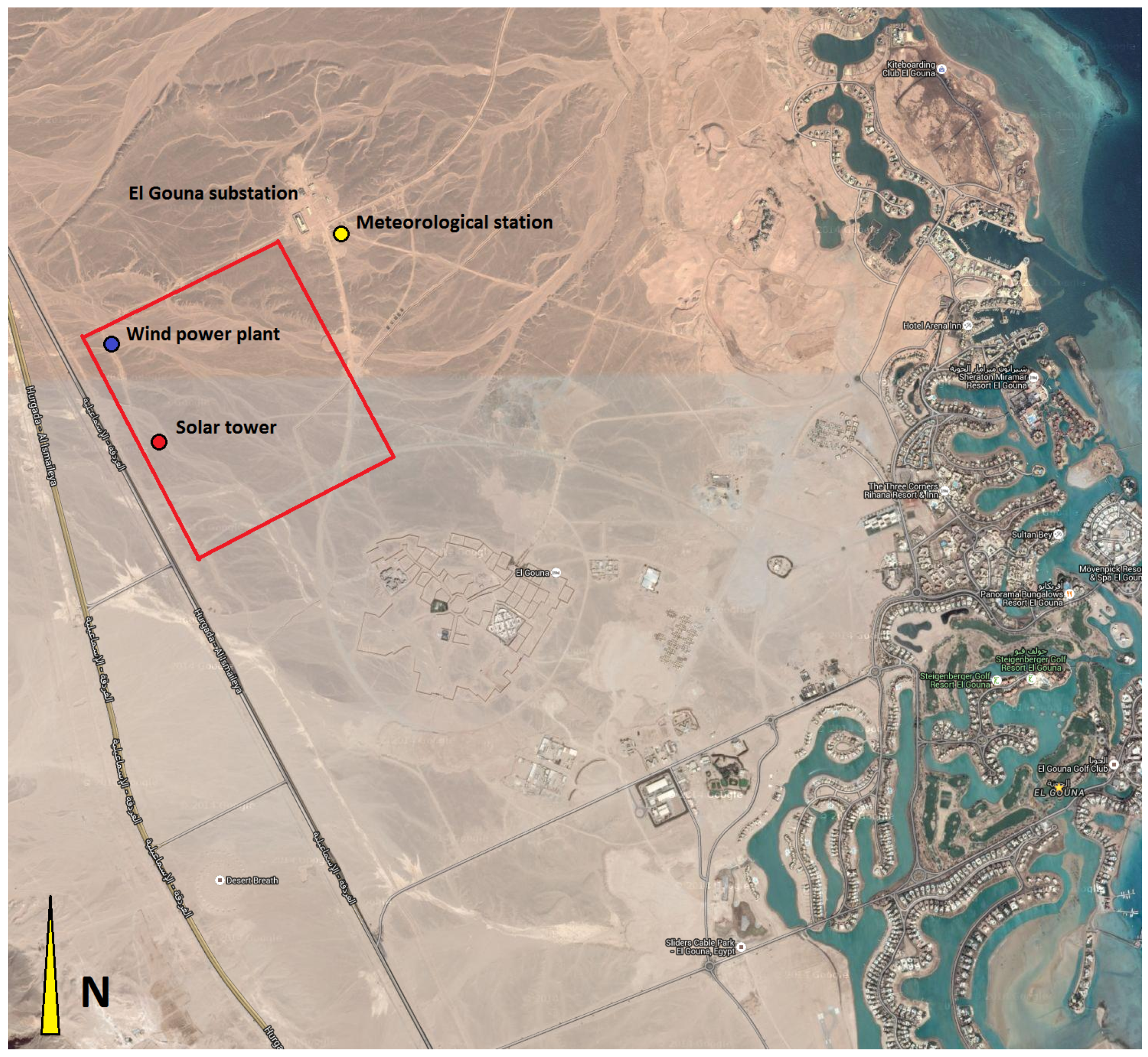
This paper focuses on the integration of a concentrating solar power (CSP) plant with attached thermal seawater desalination [3,4] into a real demand scenario of a city in Egypt and the assessment to what extent the energy and water demand can be covered by this technology. Due to the availability of meteorological [5] as well as power and water demand data [6,7], the city of El Gouna is chosen. In addition, El Gouna is heading towards becoming the first “carbon neutral” city of Africa [8]. Therefore, the overall goal should be a 100% supply with renewable energies. The financial conditions need to be carefully considered in order to evaluate the local electricity and water market for the development of respective demand scenarios.

2. Site Specific Considerations

The analysis of the meteorological data measured in El Gouna shows a high direct irradiation for the complete year favoring the power conversion in a CSP plant. The yearly precipitation has not been measured, but the literature gives negligible small amounts [9,10].

The city of El Gouna was originally planned as a tourism resort but has developed to a regular town with around 16,000 inhabitants over the last two decades. The actual power and water demand depends on the occupancy of 16 hotels. Currently, there are also about 700 privately owned mansions, 1500 apartments, about 120 restaurants, a hospital, an international school and a university campus present. The 18-hole golf course (Steigenberger Hotel) has a special influence on the irrigation water demand. The total area is covered with a vegetation amount up to 945,000 ${\mathrm{m}}^2$ [7,11].

Table 1. Power and water demand in the year 2013, El Gouna, Egypt [7,12].

Month 2013	Electricity ${\mathbf{MWh}}_{\mathbf{el}}$	Water ${\mathbf{m}}^{\mathbf{3}}$
January	6472	161,879
February	6003	144,031
March	7111	150,667
April	7739	202,654
May	9911	212,178
June	10,274	239,528
July	10,748	243,079
August	10,645	264,184
September	9051	258,147
October	8763	233,159
November	6908	205,754
December	6961	174,223
Total	100,586	2,489,483

summarizes the power and water demand of El Gouna during the year 2013.

2.1. Electricity Demand

The power demand has been covered by several Diesel generators with heavily subsidized fuel prices [7]. Since 2012, El Gouna has been connected by a high-voltage power line to the national grid of Egypt. The price for electricity is between 0.12 and 0.20 US $/kWh for the end consumers [7].

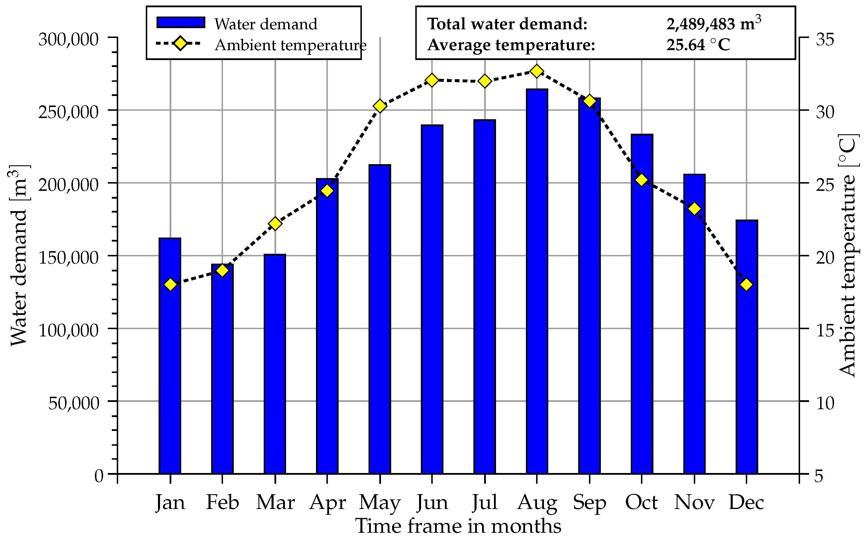
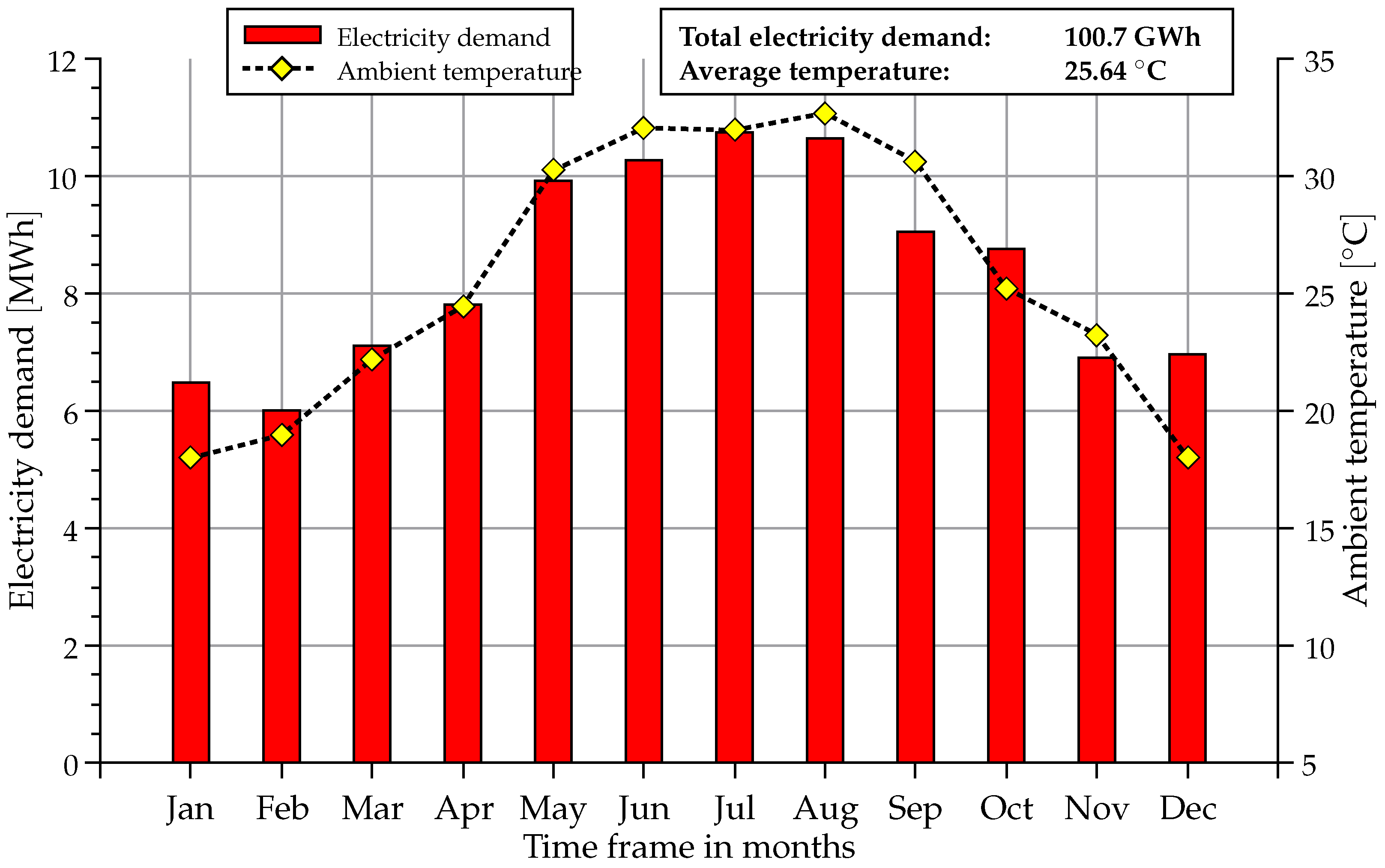
Figure 1 visualizes the electricity demand for each month during the year 2013 (for data completeness reasons, the data include March to December 2013 and January to February 2014. In the following analysis, the data is treated as from 2013). The total power consumption sums up to 100.7 ${\mathrm{GWh}}_{\mathrm{el}}$ with the lowest power demand of about 6.5 ${\mathrm{MWh}}_{\mathrm{el}}$ in the winter season (November to March) and the highest power demand of 10.5 ${\mathrm{MWh}}_{\mathrm{el}}$ during the summer season (May to August). The reason for these deviations can be mainly seen in the power demand of the air-conditioning systems of the hotels and private apartments. The assumption is proven by the strong correlation between the ambient temperature for the time period which is also visualized in Figure 1.

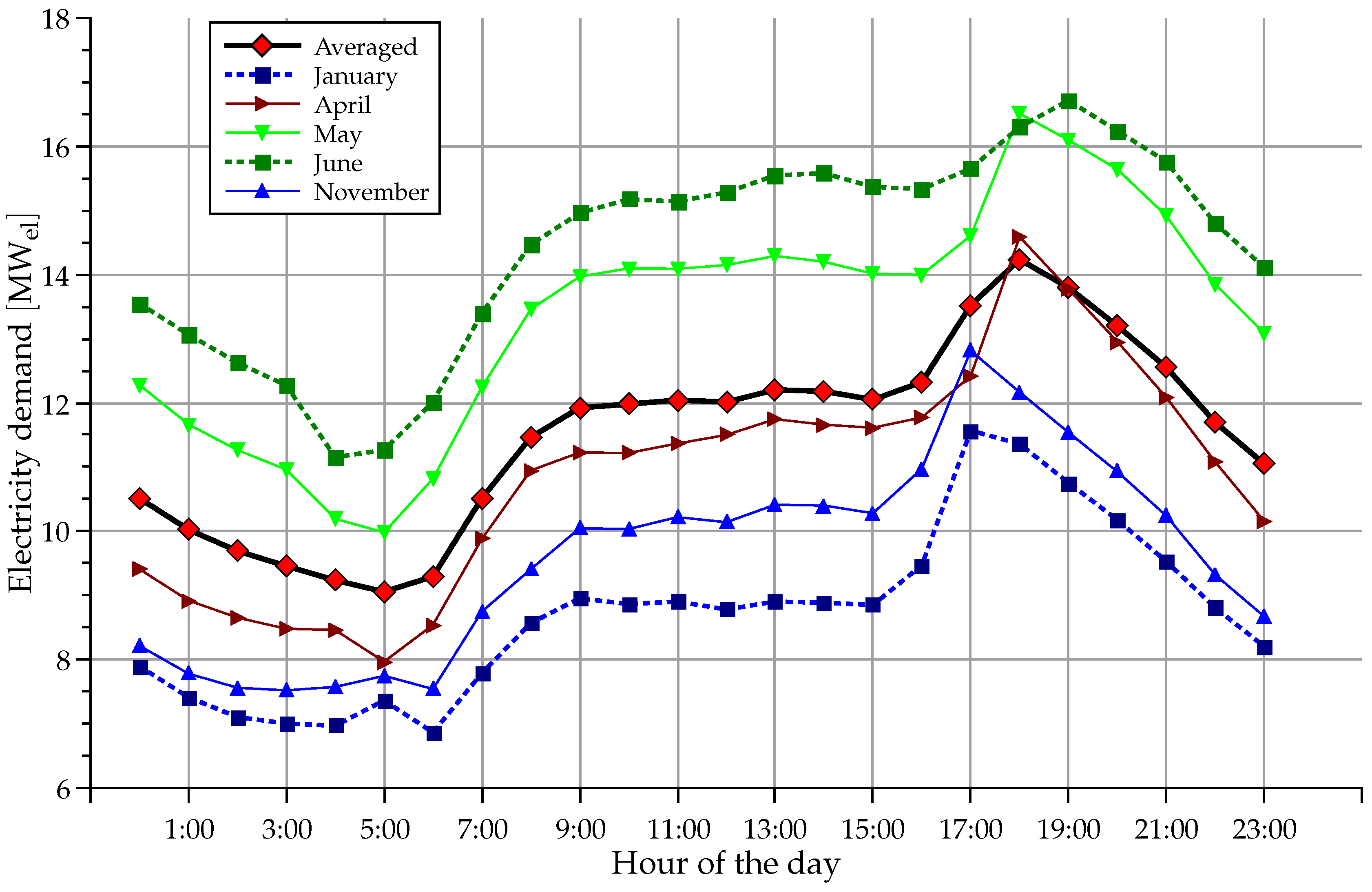
In order to model the supply scenario with renewable energies, the daily power load is of high interest. The analysis of the available data is shown in Figure 2 for each hour of the day for selected months of the year 2013. The peak loads vary strongly depending on the hour of the day. The months with the lowest consumption (January) and the highest consumption (June) are specially visualized in Figure 2. The lowest consumptions occurs during the morning hours (4:00 am to 6:00 am) while the peak demand occurs in the evening hours (5:00 pm to 7:00 pm), shown by the average power demand line. Taking the power demand curve of whole Egypt into account, it can be stated that the shape of the power demand curve is comparable to the city of El Gouna [13].

2.2. Water Demand

All available water sources in El Gouna need to be desalinated or transferred by pipelines from the Nile Delta in Lower Egypt. The second option is often disrupted and not very reliable in many districts. As a consequence of that, a huge desalination capacity is required.

In El Gouna, there is an installed desalination capacity of 9,500 ${\mathrm{m}}^3/\mathrm{d}$ for drinking water and 1500 ${\mathrm{m}}^3/\mathrm{d}$ for irrigation water. All desalination plants are working based on reverse osmosis (RO) using membranes. The intake is realized by several wells delivering brackish water from the nearby mountains with a salinity of around 7 $\mathrm{g}/\mathrm{L}\mathrm{TDS}$. Some desalination plants also use beach wells with a seawater salinity of 31to 41 $\mathrm{g}/\mathrm{L}\mathrm{TDS}$. Those plants are mostly small plants with a capacity of 500 to 1000 ${\mathrm{m}}^3/\mathrm{d}$ which are not permanently operated. They are only used if the supply from the brackish water wells is not sufficient. In total, there are eight desalination plants for saline water and seven plants for brackish water with a capacity of 5500 ${\mathrm{m}}^3/\mathrm{d}$ and 4000 ${\mathrm{m}}^3/\mathrm{d}$, respectively.

Table 2. Seawater analysis El Gouna, Red sea, [11].

Parameter	Value	Unit
pH	8.43	–
Conductivity	58.3	$\mathrm{mS}/\mathrm{cm}$
Oxygen content, O${}_2$	60.7	%
Total solids, TS	45.2	$\mathrm{g}/\mathrm{L}$
Total suspended solids, TSS	0.08	$\mathrm{g}/\mathrm{L}$
Total dissolved solids, TDS	43.7	$\mathrm{g}/\mathrm{L}$
Total organic carbon, TOC	3.64	$\mathrm{mg}/\mathrm{L}$
Anion: ${\mathrm{Cl}}^{-}$	17,189	$\mathrm{mg}/\mathrm{L}$
Anion: ${\mathrm{Br}}^{-}$	6.89	$\mathrm{mg}/\mathrm{L}$
Anion: ${\mathrm{SO}}_4^{2-}$	2897	$\mathrm{mg}/\mathrm{L}$
Cation: ${\mathrm{Ca}}^{2+}$	449	$\mathrm{mg}/\mathrm{L}$
Cation: ${\mathrm{K}}^{+}$	506	$\mathrm{mg}/\mathrm{L}$
Cation: ${\mathrm{Mg}}^{2+}$	1168	$\mathrm{mg}/\mathrm{L}$
Cation: ${\mathrm{Na}}^{+}$	1150	$\mathrm{mg}/\mathrm{L}$

shows the seawater composition. The salinity is above the average seawater with total dissolved solids of 43.7 $\mathrm{g}/\mathrm{L}\mathrm{TDS}$. Figure 3 shows the monthly water demand during the year 2013 and is similar to the electricity demand in Figure 1. The lowest demand accrues in February and the highest in August 2013, which is one month offset compared to the electricity demand. Furthermore, more than 30% of the irrigation water demand is used for the golf course.

3. Modeling of Supply and Demand

The CSP plant with integrated thermal desalination [3,4] has been dimensioned in order to cover the demand in 2013 up to 70%. Fitted with a large thermal storage system, it can been understood as the main component of the electricity and water supply system. In order to respect the future growth of El Gouna, it is expected an increasing energy demand. This demand increase shall be covered by additional renewable energies supply systems in combination with the CSP plant. One consequence is that surplus energy could be generated during the day. This surplus energy shall be stored in the thermal storage system of the CSP plant in order to extend the operation time of the CSP and thus, increase the electricity generation, the capacity factor as well as the quantity of desalinated water.

3.1. Electricity Demand Forecast

In order to consider the average future growth of the demand, the yearly demand is scaled up according to the latest available report of the Egyptian Electricity Holding Company (EEHC) [13] using the following equation:

$$D_{f,a}=D_{act}·{(1+r)}^t$$

(1)

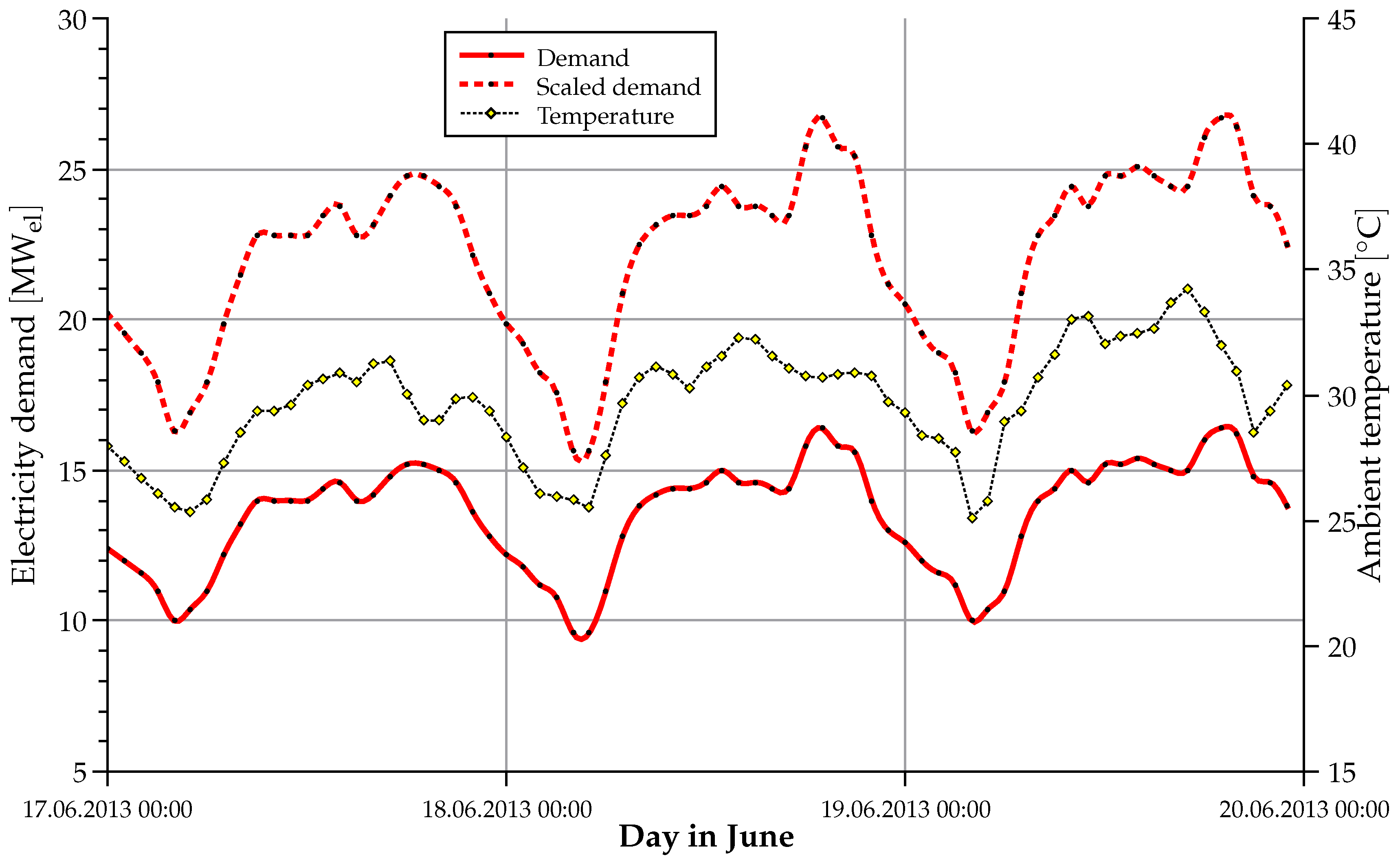
The average growth rate $\left(r\right)$ is estimated as 5% per year $\left(t\right)$ according to [13]. In order to estimate the future energy demand, $\left(t\right)$ is set to 10 years. Figure 4 maps exemplary the demand in ten years for three days of June basing on actual power demand at this day. The plotted ambient temperature shows the strong correlation between the electricity demand and the actual temperature of the particular hour of the day.

Concerning the actual power demand basing on [12] in Figure 2 during the year 2013, the CSP system has been dimensioned to supply the average electricity demand of 12 to 14 ${\mathrm{MW}}_{\mathrm{el}}$. Estimating an average growth of the electricity demand of 5% per year, it requires the building up of an additional capacity of 4 ${\mathrm{MW}}_{\mathrm{el}}$ in order to cover the average demand in the next 10 years. This shall be covered by photovoltaic and wind power plant each dimensioned with 2 ${\mathrm{MW}}_{\mathrm{el}}$.

3.2. CSP Plant with Thermal Desalination

The CSP plant is designed as solar tower plant with direct thermal storage system in order to allow for base load power supply. All performance calculations have been realized using the software Ebsilon Professional [14]. The power plant condenser is designed as interface to the desalination unit substituting the cooling system. The high efficiency of the proposed low-temperature desalination can be considered as result of the new developed spraying system which allows a direct contact condensation on sprayed droplets [15]. However, the development of this desalination system has not yet reached its full potential and proceeds continually while the newest scientific articles mentions the possibility of new applications that use this technology [16,17,18]. The numerical model of the thermal desalination unit [4,19] has been created in cooperation with the project engineers of an existing pilot plant using the kernel scripting module of Ebsilon [3,4,20]. A time series analysis of the extensive meteorological data of the given location [5] have been executed in order to determine the optimal design parameters for the plant and to calculate annual electricity and water production. All design parameters are summarized in

Table 3. Concentrating solar power (CSP) plant, design parameters.

Parameter	Symbol	Value	Unit
Gross electricity	$P_{el,gen}$	13.2	${\mathrm{MW}}_{\mathrm{el}}$
Gross water	$W_{gen}$	2250	${\mathrm{m}}^3/\mathrm{d}$
Annual electricity generation	$P_{el,a}$	100,978	$\mathrm{MWh}$
Annual water production	$W_{gen,a}$	523,385	${\mathrm{m}}^3/\mathrm{a}$
Total reflective area	$A_{ref}$	178,530	${\mathrm{m}}^2$
Total land use	$A_{tot}$	1,368,732	${\mathrm{m}}^2$
Receiver, thermal capacity	$Q_{rec}$	100	${\mathrm{MW}}_{\mathrm{th}}$
Storage, thermal capacity	$Q_{sto}$	630	${\mathrm{MWh}}_{\mathrm{th}}$
Annual DNI	$I_{DNI}$	3087	$\mathrm{kWh}/{\mathrm{m}}^2$
Solar multiple	$SM$	2.8	-
Capacity factor	$CF$	85.1	%
Full load hours	$FLH$	7448	$\mathrm{h}$

.

In a further step, the operational parameters obtained from Ebsilon have been transferred to the System Advisor Model (SAM) of NREL [21]. This software and the corresponding data library have been developed to evaluate and compare various power generation technologies. Furthermore, a special model for point focusing concentrated solar power technology utilizing thermal energy storage has been implemented. This model incorporates the knowledge of several realized projects and thus the results of a number of feasibility studies executed by different engineering consultants [21]. It is the most advanced publicly available tool for the economic evaluation of renewable power generation.

The model plant with its solar tower and heliostat field design has been optimized using the SAM data library and merged to the simulation results from Ebsilon to ensure best performance at the lowest predicted expenditures. In order to obtain more realistic results, a location data file with meteorological information [5] has been implemented in SAM [21].

3.3. Photovoltaic Model Plant

Solar energy conversion by photovoltaic panels (PV) can be considered as a commercially matured technology due to several reasons. During the last decades, the technology has been drastically improved by advanced research in material science, mainly basing on silicon and semiconductor processing industries. Improved manufacturing quality and mass production have let to cost reductions through economies of scale.

Nevertheless, the electricity generation of PV panels solely depend on the solar radiation. Thus, those systems deliver only fluctuating energy and need a compensation in times without solar radiation for a secure power supply. The combination with battery storage systems have gained more importance during the last years and can be also scaled to larger power plant. However, due to the relative low prices and strong commercialization, PV can significantly reduce the consumption of fossil energy carriers. The advantages lay in the combination with other renewable energy supply systems where PV is suitable to support the demand coverage of the modeled supply scenario.

In order to calculate the net power generation of a PV system, the solar resource and the incident angle on the PV panel are the main impact factors [22]. Due to the modeling of a heliostat field for the CSP plant, it is intended to integrate the PV panels on additional two-axis tracked heliostats directly in the solar field of the CSP plant.

The measured global horizontal irradiation $\left(G\right)$ and the sun elevation angle γ allow the calculation of the direct normal irradiation (DNI). Because a PV system also converts diffuse irradiation measured by the weather station, the calculated DNI values cannot be used directly. They need to be converted into the global tilted irradiation value GTI depending on the solar angles at the particular time of the day [23]. In order to simplify the calculation, the diffuse radiation on a horizontal plane D is normalized depending on the solar elevation angle $\left(\gamma \right)$ to the measured diffuse normal irradiation DN and added to the DNI. The calculation results in the global tilted irradiation denoted as GTI on the PV panel under the assumption that the PV panels are arranged on a two-axis tracked heliostat:

$$\begin{array}{cc}\hfill DNI& =\frac{G-D}{sin\gamma }\hfill \\ \hfill DN& =\frac{D}{sin\gamma }\hfill \\ \hfill GTI& =DNI+DN=\frac{G-D}{sin\gamma }+\frac{D}{sin\gamma }\hfill \end{array}$$

(2)

In order to respect the maximal tilt angle of the heliostats during sun rise and sun set, all sun elevation angles $\left(\gamma \right)$ below 10${}^{\circ }$ are set to zero. The resulting GTI values are significantly higher compared to the DNI values ranging up to 1100 $\mathrm{W}/{\mathrm{m}}^2$. The comparison of the calculated GTI with Meteonorm data show a sufficient correlation [9,10].

3.3.1. PV Performance Model

The calculation procedure of the net power output of the complete PV plant is adapted from [22]. In the first step, the calculation of the maximum power point voltage $\left(U_{mpp}\right)$ at given irradiation GTI is expressed in the following Equation (3). All values with the index 0 describe the reference conditions given by the manufacturer in the data sheet of the PV panel:

$$U_{mpp}=U_{mpp,0}·\frac{lnGTI}{lnGT{I}_0}$$

(3)

where the same applies for the maximum power point current $\left(I_{mpp}\right)$ at irradiation level depending on the GTI:

$$I_{mpp}=I_{mpp,0}·\frac{GTI}{GT{I}_0}$$

(4)

The PV panel heats up during operation which has a diminishing effect to the power output. Usually, the effect is expressed by the heat-up coefficient $\left({\tau }_{PV}\right)$ which is given in K per solar irradiation using the unit $\frac{\mathrm{K}}{\mathrm{W}/{\mathrm{m}}^2}$. The temperature of the PV panel $\left(T_{PV}\right)$ consequently calculates to:

$$T_{PV}=T_{amb}+GTI·{\tau }_{PV}$$

(5)

In order to calculate the maximum power point output $\left(P_{mpp}\right)$ of the complete array, the number of PV panels switched in series $\left(n_s\right)$ and in parallel $\left(n_p\right)$ need to be multiplied by the temperature correction term. The manufacturer gives a coefficient for the thermal properties of the PV panel $\left({\alpha }_{mpp}\right)$ and usually given in $\%/\mathrm{K}$:

$$P_{mpp}=n_s·n_p·U_{mpp}·I_{mpp}(1+{\alpha }_{mpp}·(T_{PV}-T_{amb}))$$

(6)

The power output of the complete PV system is additionally influenced by three main losses which are given by efficiencies factors $\left(\eta \right)$. The panel soiling $\left({\eta }_{soil}\right)$ respects the power reduction due to opacity. Possible AC-DC inverter losses are respected by $\left({\eta }_{inv}\right)$ and the total field efficiency is respected by $\left({\eta }_{fld}\right)$. In summary of the Equations (3-6), the total power output of the PV system calculates like the following:

$$P_{PV,net}=P_{mpp}·{\eta }_{soil}·{\eta }_{inv}·{\eta }_{fld}$$

(7)

3.3.2. Specification of the PV Module

Due to the abundant presence of possible manufacturers, a standard module from the renown company BOSCH GmbH [24] has been chosen. It is a crystalline silica based solar module which has a high processing quality and long-term stable power output. One module consists of 60 mono-crystalline solar cells mounted to a black anodized aluminum frame. Each PV module has a dimension of 1660 × 4990 $\mathrm{mm}$ for one PV module. The operating temperature is given by the manufacturer in the limit from −40 to +85 °C. The soiling factor $\left({\eta }_{soil}\right)$ assumes a clean condition and an inverter efficiency has been chosen with 96% efficiency.

Table 4. Photovoltaic panels (PV) module characteristics [24].

Parameter	Symbol	Value	Unit
Type and model number	BOSCH c-Si M60S	M245	-
Maximum power point output	$P_{mpp}$	245	$\mathrm{W}$
Maximum power point voltage	$U_{mpp}$	30.11	$\mathrm{V}$
Maximum power point current	$I_{mpp}$	8.14	$\mathrm{A}$
Temperature coefficient	${\alpha }_{mpp}$	-0.44	$\%/\mathrm{K}$
Module area	$A_{pv,m}$	1.64	${\mathrm{m}}^2$
Heat-up gradient	${\tau }_{pv}$	0.04	$\mathrm{K}/\mathrm{W}/{\mathrm{m}}^2$
Soil factor	${\eta }_{soil}$	96	%
Inverter efficiency	${\eta }_{inv}$	96	%
Field efficiency	${\eta }_{fld}$	98	%

summarizes all parameters at reference conditions of $GT{I}_0=1000\mathrm{W}/{\mathrm{m}}^2$ and $T_{amb,0}=25$ °C.

3.3.3. Dimensioning of the PV Model Plant

Knowing the characteristics of one single PV module and its power output allows for the calculation of the total power output of the PV model plant. In order to integrate the system in the CSP heliostat field, the capacity is limited to 2 ${\mathrm{MW}}_{\mathrm{el}}$ at nominal conditions. The capacity requires the deployment of 8800 PV modules using the properties of Table 4. One CSP heliostat fitted with mirrors has a reflective surface of 100 ${\mathrm{m}}^2$. Theoretically, the replacement of the mirrors with PV modules would allow for 60 PV modules on one heliostat. To respect the possible additional weight of the PV modules, it is calculated with 55 PV modules per heliostat $\left(n_s\right)$. All modules on the heliostat are electrically switched in series. The number of heliostats fitted with 55 PV panels $\left(n_p\right)$ and are switched in parallel. The total array sums up to a nominal power generation of 2.16 ${\mathrm{MW}}_{\mathrm{el}}$ at peak. The calculation results of the complete PV model plant are summarized in

Table 5. PV model plant, system parameters.

Parameter	Symbol	Value	Unit
Heliostats with PV modules, in parallel	$n_p$	160	-
PV modules per heliostat, in series	$n_s$	55	-
MPP voltage, system	$U_{mpp,0,sys}$	1656	$\mathrm{V}$
MPP current, system	$I_{mpp,0,sys}$	1302	$\mathrm{A}$
MPP power, system	$P_{mpp,0,sys}$	2157	$\mathrm{kW}$
PV system, total aperture area	$A_{pv,sys}$	14462	${\mathrm{m}}^2$
Annual power generation, total plant	$P_{tot,pv}$	5948	$\mathrm{MWh}$
Annual power generation, per heliostat	$P_{hel,pv}$	37	$\mathrm{MWh}$
Total number of heliostats (CSP and PV)	$n_{tot}$	1943	-

.

3.4. Wind Model Plant

The wind power technology can be considered as fully commercialized. However, the Red Sea coast of Egypt is one of the windiest regions of Egypt. However, wind power supply is also considered as a fluctuating energy resource which strongly depends on the available wind speed at the given location. Here, just one exemplary wind turbine with an installed capacity of 2 ${\mathrm{MW}}_{\mathrm{el}}$ is modeled in order to support the supply scenario.

The mechanical power $\left(P_w\right)$ from a wind turbine depends on four main factors, which are the prevailing wind speed $\left(v_w\right)$, the rotor area $\left(A_{ro}\right)$, the power coefficient $\left(c_b\right)$ and the density of the air $\left({\rho }_{air}\right)$:

$$P_w=\frac{1}{2}{\rho }_{air}·c_b·A_{ro}·v_w^3$$

(8)

While the density of the air $\left({\rho }_{air}\right)$ and the wind speed $\left(v_w\right)$ depend on the ambient conditions, the other factors are influenced by the dimension and the design of the wind turbine. Especially at low wind speeds, the power coefficient $\left(c_b\right)$ strongly influences the power output and can theoretically not exceed more than 59.3%. This factor is also called Betz-coefficient and can be derived from the fluid mechanics and the conservation of momentum. The strongest influence on the power output has the prevailing wind speed $\left(v_w\right)$ in the rotor plane due to the multiplication in the cube (Equation (8)). All data used for the calculation have been measured by the meteorological station [5].

3.4.1. Wind Performance Model

The wind performance model is adapted from [25]. In order to calculate the net power output from a given wind turbine, the measured wind speed needs to be corrected according to the rotor height. The hourly wind data [5] is measured at a given height $h_1=10\mathrm{m}$. The measured wind speed is denoted as $v\left(h_1\right)$ in $\mathrm{m}/\mathrm{s}$. Furthermore, the available wind speed at rotor height $v\left(h_2\right)$ depends on the surrounding area which is expressed by a ground roughness factor $\left(z_0\right)$. Obstacles like bushes, trees and buildings are causing turbulences which reduce the power output of the wind turbine. Equation (9) is used to calculate the wind speed at the rotor height $v\left(h_2\right)$:

$$v\left(h_2\right)=v\left(h_1\right)·\frac{ln\left({\displaystyle \frac{h_2-d}{z_0}}\right)}{ln\left({\displaystyle \frac{h_1-d}{z_0}}\right)}$$

(9)

The height of possible obstacles d near the measurement can be used for the calculation given in Equation (9). Because of the selected location in desert land, there are no obstacles neither near the meteorological station nor at the foreseen location of the wind turbine. Therefore, d is set to zero.

In a next step, the density of the air $\left({\rho }_{air}\right)$ needs to be corrected. It has a linear effect to the power output of the wind turbine. The density is mainly affected by the atmospheric pressure, the elevation and the ambient temperature. In this model, the effect is respected by a factor $\left({\eta }_{den}\right)$ which is calculated as follows:

$${\eta }_{den}=\frac{{\rho }_{air}}{{\rho }_0}=\frac{p_{amb}·(t_0+273.15)}{p_0·(t_{amb}+273.15)}$$

(10)

The values with the index 0 in Equation (10) represent the reference conditions. The reference conditions are assumed with the temperature $t_0=20{}^{\circ }\mathrm{C}$, the pressure $p_0=1013\mathrm{mbar}$ and the density ${\rho }_0=1.255\mathrm{kg}/{\mathrm{m}}^3$.

3.4.2. Specification of the Wind Turbine

In order to calculate the additional power generation of a wind turbine, one turbine from one of the available wind turbine manufacturers can be specified. In this study, a turbine from Enercon GmbH is selected [26]. All parameters and site specific characteristics are summarized in

Table 6. Wind turbine properties and site characteristics [26].

Parameter	Symbol	Value	Unit
Type and model number	ENERCON	E-82	-
Nominal power capacity	$P_{nom}$	2050	$\mathrm{kW}$
Start up wind speed	$v_{in}$	3.5	$\mathrm{m}/\mathrm{s}$
Nominal wind speed	$v_{nom}$	13	$\mathrm{m}/\mathrm{s}$
Shut-down wind speed	$v_{out}$	25	$\mathrm{m}/\mathrm{s}$
Rotor height	$h_2$	78	$\mathrm{m}$
Roughness index	$z_0$	0.03	$\mathrm{m}$
Grid connection efficiency	${\eta }_{con}$	96	%

.

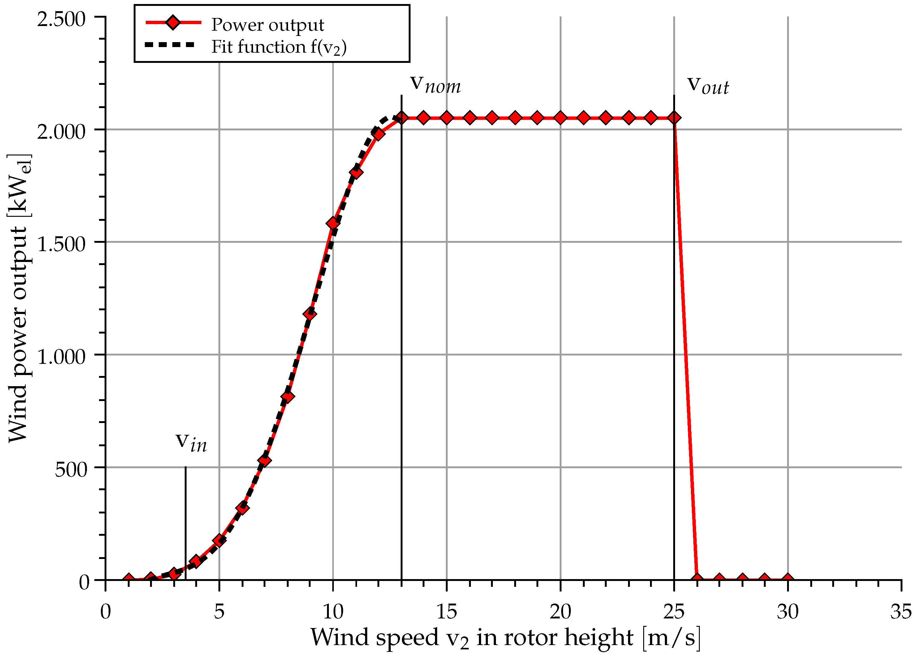
For the calculation of the power output depending on the actual wind speed in rotor height $\left(h_2\right)$, the characteristic power curve needs to be interpolated. The start-up (or cut-in) wind speed $\left(v_{in}\right)$ can be considered as the minimal wind speed for power generation. The nominal power output according to the design capacity is reached at the nominal wind speed $\left(v_{nom}\right)$. The range of the wind speed between $\left(v_{in}\right)$ and $\left(v_{nom}\right)$ requires constant blade adjustment (pitch). In order to avoid mechanical damage, the wind turbine is shut down at the maximum wind speed $\left(v_{out}\right)$ and parked in a safe position.

Figure 5 shows the development of the power curve with the mentioned design-depending wind speeds. The manufacturer provides a detailed power curve for each wind speed according to the selected turbine E-82 [26]. The modeling of the power output depending on the prevailing wind speed in the rotor height $\left(v_2\right)$ requires the adaption of a fit function. However, a polynomial function of the fourth order denoted as $f\left(v_2\right)$ can be used to fit the course of the power function between $\left(v_{in}\right)$ and $\left(v_{nom}\right)$ given by the manufacturer [26]. The fit function is visualized in Figure 5 by a dotted black line. Equation 11 has been developed to ensure a correlation coefficient $R^2=0,999$ to the manufacturer data:

$$f\left(v_2\right)=-0.579v_2^4+13.736v_2^3-85.231v_2^2+231.86v_2-220.47$$

(11)

The complete wind power curve in Figure 5 is modeled according to the Equation (12). The units are given in ${\mathrm{kW}}_{\mathrm{el}}$ for $\left(P_{E82}\right)$ and in $\mathrm{m}/\mathrm{s}$ for $\left(v_2\right)$, respectively:

$$P_{E82}\left(v_2\right)=\left\{\begin{array}{cc}0\hfill & \mathrm{if}{v}_2<v_{in}\hfill \\ f\left(v_2\right)\hfill & \mathrm{if}{v}_{in}<v_2<v_{nom}\hfill \\ 2050\hfill & \mathrm{if}{v}_{nom}<v_2<v_{out}\hfill \\ 0\hfill & \mathrm{if}{v}_2>v_{out}\hfill \end{array}\right.$$

(12)

Summarizing, the wind power output $\left(P_w\right)$ is lowered by the correction factor for the air density $\left({\eta }_{den}\right)$ according to ambient pressure and temperature (Equation (10)) as well as the efficiency of the power connection to the grid $\left({\eta }_{con}\right)$. Equation (13) shows the relation:

$$P_w=P_{E82}\left(v_2\right)·{\eta }_{den}·{\eta }_{con}$$

(13)

4. Storage of Surplus Power by Heat

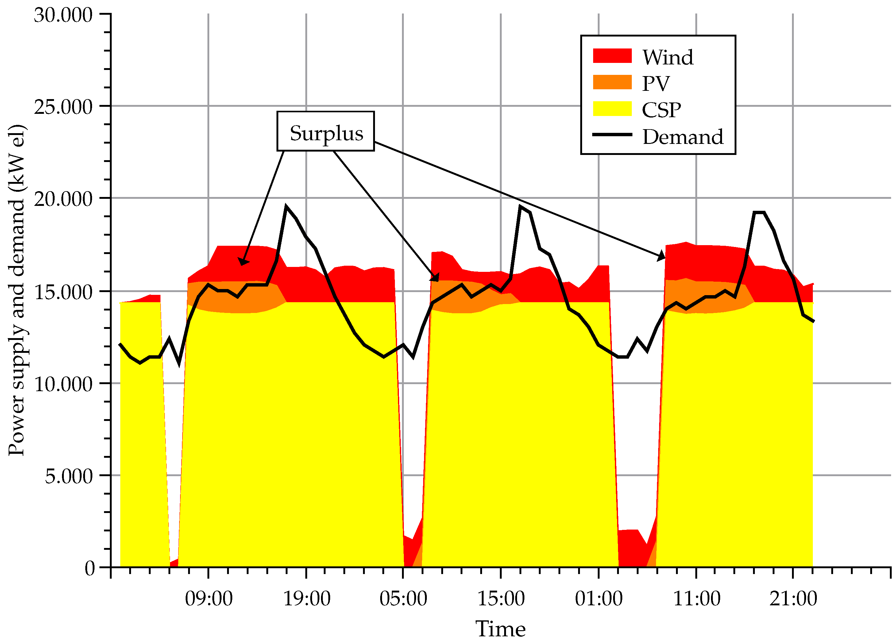
It can be expected that the power generation of a CSP plant in connection with PV and wind power exceeds the electricity demand at certain time steps depending on environmental conditions. The total installed capacity sums up to 18 ${\mathrm{MW}}_{\mathrm{el}}$ while 14 ${\mathrm{MW}}_{\mathrm{el}}$ are maximal covered by the CSP plant and 4 ${\mathrm{MW}}_{\mathrm{el}}$ by PV and wind power. Like discussed before, only the CSP with the thermal storage can supply power on demand depending on the actual storage level. The PV and wind power plant are completely depending on the environmental resources.

Figure 6 visualizes the problem for three days in February, by hourly time steps. Especially during the day, the modeled system generates surplus power which exceeds the given electricity demand. Generally, there are several options for the handling of surplus power which are explained as follows:

• Avoiding surplus power: In the best case, the generation of surplus power could be avoided through optimal design. The design of the CSP with the thermal desalination unit allows a flexible condensation pressures which shift the power generation to more water production [3,4]. Due to the fact, that water can be easily stored, the surplus electricity generation could be reduced to a certain extent. In this study, the condensation pressure and thus, the energy and water cogeneration ratio is kept fixed for the whole year. Another option would be the supply of the RO desalination plants with the surplus power, but the operation of RO plants with variable loads are also technical challenging.
• Grid feed: Because of the existing high-voltage line to the national grid of Egypt, the generated surplus electricity could be transferred to the national network. Having an increasing amount of fluctuating renewable energy sources connected to the national grid, creates a problem for existing power plants powered by fossil fuels, with have significant time delays to react on changed load conditions. In addition to that, the operation in part-load causes reduced efficiencies in energy conversion. The problem intensifies with an increasing amount of fluctuating renewable energy sources in the national grid.
• Storage of surplus power: Another possible solution could be the conversion of the surplus power into usable heat in the thermal storage system of the CSP plant. This would extend the run-time of the CSP plant during night-operation. In most cases, the conversion of electricity into heat in power systems does not make sense, but with an increasing amount of fluctuating renewable energy sources like PV and wind power in electricity grids, the thermal storage of surplus power needs to be discussed again.

However, the existence of a large thermal storage in combination with a steam cycle power block gives the option to load the storage using surplus energy generated by fluctuating resources. Technically, it can be expressed by heating up the molten salt using an electric heater powered by surplus power to load the thermal storage during hours when the supplied power exceeds the demand. Variable loads of the electrical heater during short operation times is technically possible and always allows a high conversion efficiency. The modeled fluctuating resources in this case study are rather small dimensioned and designed to generally minimize surplus power, but the theoretical approach is outlined shortly.

4.1. Theoretical Model of Power to Heat Conversion

The relation between the available heat $\left(Q\right)$ depends on the temperature difference $\Delta T=T_2-T_1$, the specific heat capacity of the fluid $\left(c_p\right)$ and the mass flow $\left(\dot{m}\right)$ of the fluid:

$$Q=m·c_p·(T_2-T_1)$$

(14)

The considered fluid is defined as the molten salt of the thermal storage system. The conversion of the surplus power to the heat $\left(Q_{sp}\right)$ is assumed to be ideal. So the available heat is equal to the generated surplus power. The temperature difference $\Delta T$ is the temperature difference of the two molten salt storage tanks, thus defining the temperatures for the hot tank $\left(T_{sto,h}\right)$ and for the cold tank $\left(T_{sto,c}\right)$ which have a fixed $\Delta T=280\mathrm{K}$. The specific heat capacity $\left(c_{p,ms}\right)$ of the molten salt can be found in available literature and is assumed with $c_{p,ms}=1.538\mathrm{kJ}/\mathrm{kg}\mathrm{K}$ [27,28]. Rearranging Equation (14) to the mass flow of the molten salt, results in the following Equation (15) to calculate the additional mass flow $\left({\dot{m}}_{a,ms}\right)$ in the hot tank depending on the surplus power $\left(Q_{sp}\right)$:

$${\dot{m}}_{a,ms}={\displaystyle \frac{{\dot{Q}}_{sp}}{c_{p,ms}·(T_{sto,h}-T_{sto,c})}}$$

(15)

The calculation neglects possible heat and pressure losses as well as required pumping power to supply the molten salt from the cold tank to the hot tank. While the heat losses strongly depend on the technical issues, the pumping power can be estimated around 20 ${\mathrm{kW}}_{\mathrm{el}}$ based on the simulation results of the CSP plant.

5. Results of Renewable Energy Integration

5.1. Economic Assumptions

One common approach is the use of the levelized cost of electricity (LCOE) to compare different renewable energy technologies [29,30]. The LCOE is defined as the total lifetime expenditures of the plant divided by the total power generation during this time frame. The total lifetime expenditures are composed of the capital costs $C_t$, the operation and maintenance costs $O\&M_t$ and the fuel costs $F_t$ for each year. The total power generation is noted with $P_t$ and discounted using the interest rate $i_r$ for the complete plant lifetime $t_c$. Equation (16) summarizes the calculation of the LCOE:

$$LCOE=\frac{{\displaystyle \sum _{t=1}^{t_c}}\frac{C_t+O\&M_t+F_t}{{(1+i_r)}^t}}{{\displaystyle \sum _{t=1}^{t_c}}\frac{P_t}{{(1+i_r)}^t}}$$

(16)

As the proposed plant also produces water, the levelized costs of water need to be introduced. The calculation can be compared to the LCOE calculation. In the literature it is also referred as levelized water cost LWC [31]. The calculation consists of the total lifetime cost of the desalination plant divided by the total gross water production in Equation (17). The parameters are identical compared to the given definitions except from the total water production $W_t$.

$$LWC=\frac{{\displaystyle \sum _{t=1}^{t_c}}\frac{C_t+O\&M_t+F_t}{{(1+i_r)}^t}}{{\displaystyle \sum _{t=1}^{t_c}}\frac{W_t}{{(1+i_r)}^t}}$$

(17)

The most interesting factor in the calculation of LWC is the fuel cost $F_t$. Its definition is crucial for the results and is also depending on the examined technology. Basically, it accounts for the energy demand assigned to the water production and can be considered as major cost factor for desalination.

The LCOE and the LWC are widely used to compare different renewable energy and water treatment technologies with each other. Mostly, the investment decisions depend on low levelized costs neglecting other relevant dimensions such as security of supply or social aspects. The definition may be sufficient for the assessment of fossil fuel powered plants where the fuel costs account for more than 70% of the total lifetime costs. Since the selected system consists of a CSP plant with an integrated high capacity thermal energy storage system, the LCOE and LWC is a valid option to evaluate the economic feasibility of the model plant. It also ensures the comparability of the results to other technical solutions. All financial boundary conditions for the economic calculation are summarized in

Table 7. Economic boundary parameters.

Parameter	Symbol	Value	Unit
Weighted averaged capital costs	$WACC$	8	%
Interest rates	$i_r$	10	%
Operation and maintenance	$O\&M$	2.5	%
Inflation rate	$IR$	2.5	%
Plant lifetime	t	20	$\mathrm{a}$
CAPEX, CSP plant	$C_{CSP}$	140.4	$\mathrm{mil}\$$
CAPEX, PV plant	$C_{PV}$	8.4	$\mathrm{mil}\$$
CAPEX, Wind plant	$C_W$	5.3	$\mathrm{mil}\$$
Total initial cost, complete system	$C_{TOT}$	154.2	$\mathrm{mil}\$$

.

The cost structure of operational expenditures (OPEX) for the solar tower system is defined as the variable costs of power generation, maintenance cost and personnel expenses. They are usually calculated as a percentage of the CAPEX. The main operational costs of the solar power plant can be expected from the heliostat field maintenance. This includes mainly mirror cleaning and replacement as well as maintenance of the 2-axis tracking system. The influence of dusty ambient conditions (sand storms) and occasionally high wind loads has not been investigated yet. The empirical values from the literature range between 2% for large scale plants and 2.5% for small scale plants [32,33,34]. As the examined model plant can be considered as a small scale plant, the operational expenditures of 2.5% of the total investment are considered annually in all calculations for the model plant. For low temperature distillation, the operational expenditures are comparatively low for a desalination system. They can be considered annually about 1.5% of the CAPEX [16]. Since the low temperature desalination works by the mechanisms of thermal treatment at low temperatures and pressures, the designed heat exchange parameters need to be maintained.

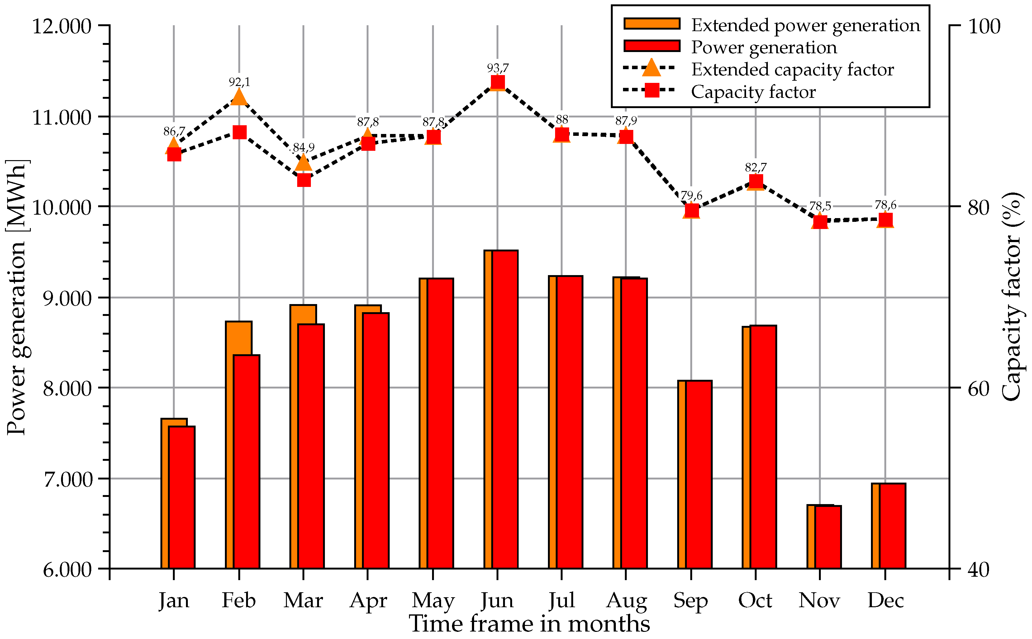
5.2. Power and Water Supply by CSP Plant

The evaluated CSP plant with its 13.2 ${\mathrm{MW}}_{\mathrm{el}}$ design capacity can supply in average around 60% of the scaled electricity demand in the next ten years. The lowest monthly coverage of 53% occurs in July and August during high-season time. During January to March, the monthly coverage is increased and ranges between 72% up to 85%.

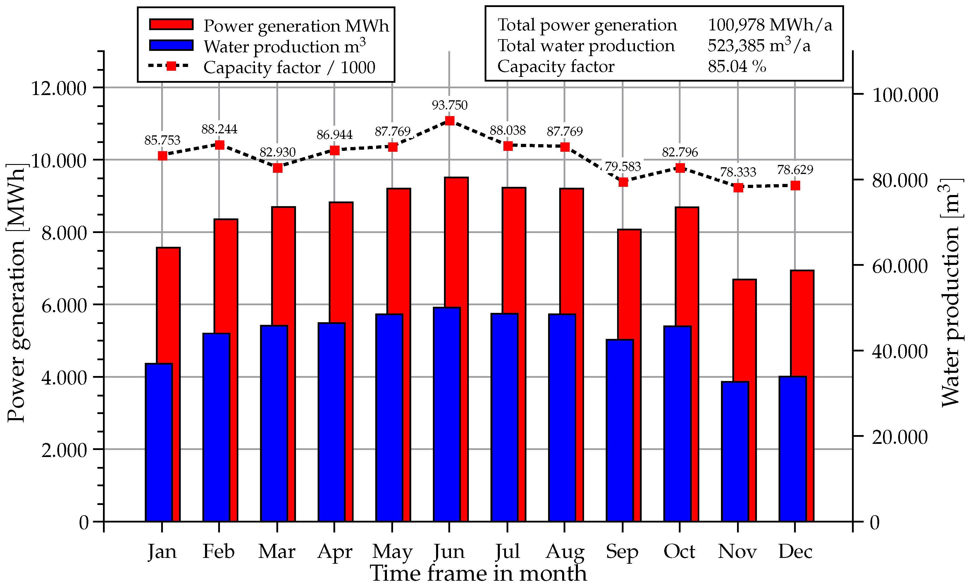
Figure 7 presents the power and water production for one year of the CSP plant with attached thermal desalination unit. The total power generation ranges between 6700 up to 9500 ${\mathrm{MWh}}_{\mathrm{el}}$ per month. The achievable capacity factors of the CSP plant is between 78% in December and up to 93% in June. It is important to mention that the operation time of the CSP always covers the peak demands in the evening hours (5:00 pm to 7:00 pm), which has been analyzed in Section 2.1 and Figure 2. The shut-down time of the CSP plant is during low-loads (4:00 am to 6:00 am), depending on the respective level of the thermal storage.

For the time period from November to February, the plant operates in part-load with 83% in order to extend the operation time during the hours without solar irradiation. October 2013 has been a more sunny month compared to September of the same year, which results in a higher power generation as well as capacity factor. Furthermore, the lowest month for power generation is November, which is due to short day length and thus reduced irradiation. The occurrence of cloudy days is also raised limiting the available direct normal irradiation.

Throughout the year, the water production covers only around 20% of the fresh water demand [6]. Due to the fixed operating point and optimized cogeneration ratio, the water production always shares a constant portion of the electricity generation. The monthly coverage ranges between 16% in November and 31% in February. The water production and the total share can be easily increased by changing the condensation pressure of the CSP plant. In the examined case, the condensation pressure is kept constant at 0.14 $\mathrm{bar}$.

5.2.1. Costs of CSP Model Plant

The cost allocation in cogeneration plants has a strong influence on the evaluation of technical solutions and the discussed plant designs. The literature gives several approaches for the respective cost allocation and are abundantly applicable for electricity and water generation. In the present study, the reference cycle costing method has been chosen. The method bases on the comparison with a reference plant to allocate the fuel costs. The plant performance operated in cogeneration is compared with a single purpose plant for one product. This is called the reference cycle. For example, the cost of heat used to operate the desalination plant is calculated as the loss of electricity output in comparison to pure electricity generation. This approach is also known as the lost kilowatt method and has been proposed in international publications [31,35,36,37,38]. All data used for the economic calculation have been summarized in Table 3 and Table 7. The specific CAPEX can be given with 10,640 $\$/{\mathrm{kW}}_{\mathrm{el}}$ which seems to be quite high. The reason can be found in the large thermal storage system in combination with the solar field. Nevertheless, a comparison with literature data for the plant size shows a sufficient accordance [39].

The calculation of LCOE and LWC allows two possible methods. As the desalination system replaces the conventional power plants cooling system, the investments can be calculated as one complete investment. It results in a lowered total CAPEX and thus in a lowered LWC.

Table 8. Levelized product costs for the CSP plant per year.

	Single Investment	Combined Investment	Unit
Levelized cost of electricity (LCOE)	18	18	ct$/\mathrm{kWh}$
Levelized cost of water (LWC)	2.99	2.49	$\$/{\mathrm{m}}^3$

summarizes both calculations for a “single investment” considering two separate investments for power and desalination plant, while “combined investment” describes the approach considering an integrated investment cost for the power plant and the desalination system.

5.3. Power Supply by PV and Wind Power Plant

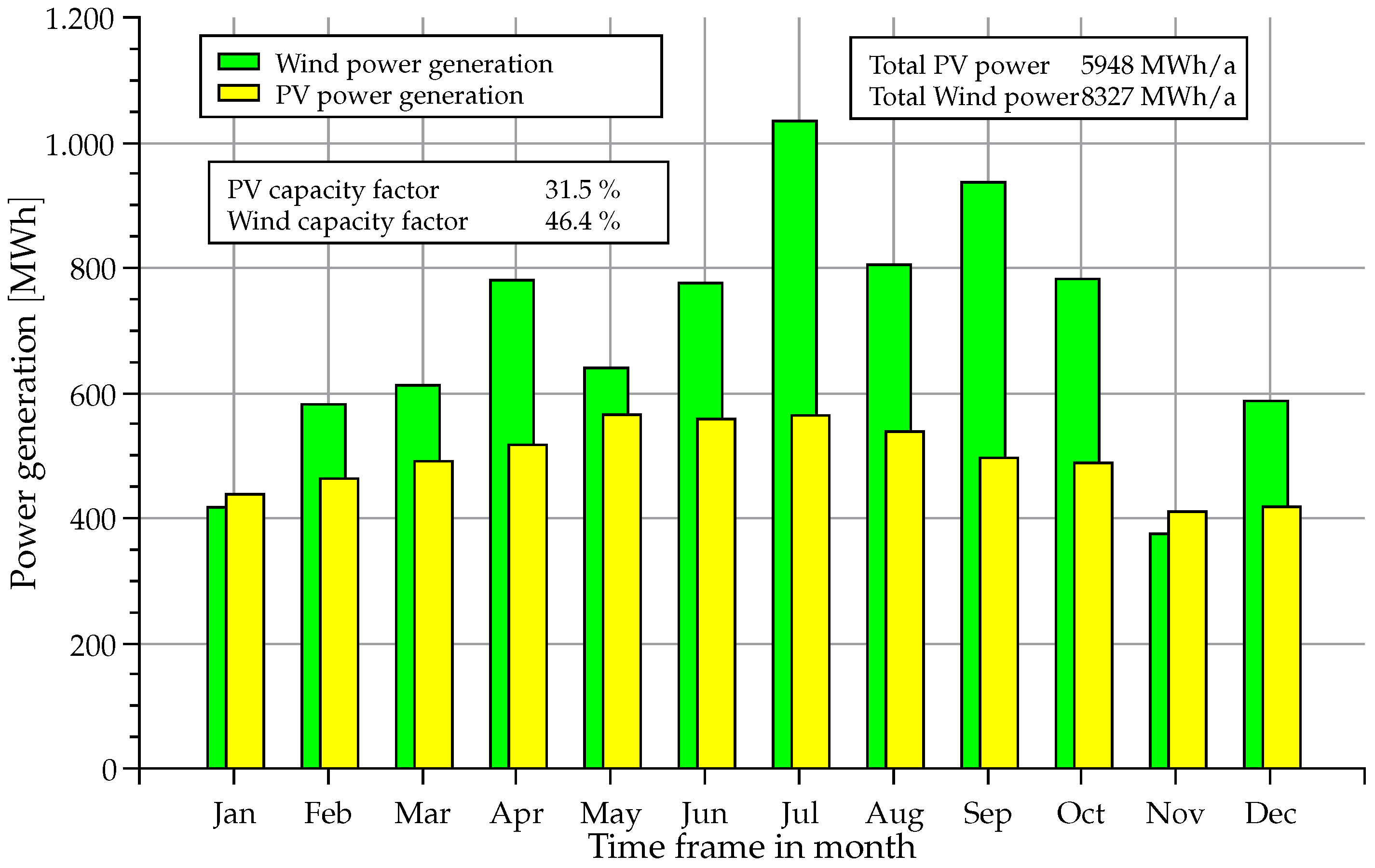
The deployment of additional 2 ${\mathrm{MW}}_{\mathrm{el}}$ capacity by a PV and 2 ${\mathrm{MW}}_{\mathrm{el}}$ by a wind power plant extends the supply and thus the demand coverage. Due to the relative small size of the systems, they can be completely integrated on the land area of the CSP plant. In addition, the comparison of two different technologies in total power generation in the selected location is easily possible. It can be expected that the generated surplus energy is also increased.

Figure 8 shows the total power generation which depends on the actual solar irradiation on a tilted surface (GTI in Section 3.3) and the prevailing wind speed measured by the meteorological station [5]. Furthermore, the results in Figure 8 also show that the installed wind power plant provides a significantly higher capacity factor compared to the PV model plant. While the PV plant achieves a total capacity factor of 31.5%, the wind power plant reaches up to 46.4%. It can be concluded that the selected location is more suitable for wind power generation. The months with the lowest power generation for both plants are November and January, reaching a combined power generation from 810 up to 870 ${\mathrm{MWh}}_{\mathrm{el}}$. However, the most yielding months are July to October, achieving a monthly power generation from 1310 up to 1640 ${\mathrm{MWh}}_{\mathrm{el}}$.

The economic analysis needs a more differentiated evaluation due to the different characters of PV and wind power generation. Both calculations are performed using the System Advisory Model (SAM) [21] described in Section 3.2. In order to derive a brief estimation of financial parameters, the PV and wind design data (see Section 3.3 and Section 3.4) are transferred to SAM.

5.3.1. Costs of PV Model Plant

Generally, the costs of the PV modules are expected to decrease in future [40,41]. Due to strong effects of economies of scale, efficiency gains in manufacturing, development of new PV technologies and the global competition, the prices for PV modules are declining and have dropped to 1050 $\$/\mathrm{kW}$ in the year 2012. The installed system costs for commercial c-Si PV systems sums up to 4590 $\$/\mathrm{kW}$ including additional heliostats (2-axes trackers), power inverters, installation overheads and site preparation [40]. Assuming an installed PV capacity of 2.16 ${\mathrm{MW}}_{\mathrm{el}}$, the total costs for this PV plant could be estimated as 9.91 $\mathrm{mil}\$$.

The calculation using SAM provides a more detailed analysis and are presented in

Table 9. PV model plant, economic data.

Parameter	Symbol	Value	Unit
Annual energy	$P_{PV,tot}$	6335	${\mathrm{MWh}}_{\mathrm{el}}$
Capacity factor	$C{F}_{PV}$	0.33	$[-]$
First year kWhAC/kWDC	$P{V}_{gen}$	2967	$\mathrm{kWh}/\mathrm{kW}$
Levelized cost (nominal)	$LCO{E}_{PV,n}$	21	ct$/\mathrm{kWh}$
Levelized cost (real)	$LCO{E}_{PV,r}$	17	ct$/\mathrm{kWh}$
Electricity cost savings	$S_{PV}$	477	$
Net present value	$B_{PV}$	−12.499	$\mathrm{mil}\$$
Total initial cost	$C_{PV}$	8.392	$\mathrm{mil}\$$

. It shows the levelized cost of electricity (LCOE) and gives an overview about the expected costs for a period of 20 years without feed-in tariffs or other governmental incentives. The results represent the total costs of the PV system also containing expenses for O&M which have been estimated to 30 $\$/{\mathrm{kW}}_{\mathrm{el}}$ [42]. The total investment including labor and site preparation sum up to 8.392 $\mathrm{mil}\$$. Overall, the resulting $LCO{E}_{PV}$ ranges between 17–21 ct$/\mathrm{kWh}$ while the nominal $LCO{E}_{PV,n}$ also respects a discount rate for inflation.

5.3.2. Costs of Wind Model Plant

Generally, the energy generation using wind power plants can be considered as technically matured and highly commercialized [43]. The effects to the economic parameters depend mainly on the location and the prevailing wind speed. The literature provides data for installed wind power capacity around 1000–2000 $\$/\mathrm{kW}$ for onshore applications [42,44,45]. Due to the installation of one single turbine without the effects of economies of scale, the costs are estimated as 2000 $\$/\mathrm{kW}$ for this study. However, the total investment costs is estimated as 4,1 $\mathrm{mil}\$$.

Table 10. Wind model plant, economic data.

Parameter	Symbol	Value	Unit
Annual energy	$P_{W,tot}$	8,539	${\mathrm{MWh}}_{\mathrm{el}}$
Capacity factor	$C{F}_W$	0.47	$[-]$
Levelized cost (nominal)	$LCO{E}_{W,n}$	1.21	ct $/\mathrm{kWh}$
Levelized cost (real)	$LCO{E}_{W,r}$	0.98	ct $/\mathrm{kWh}$
Net present value	$B_W$	-1003.95	$\mathrm{mil}\$$
Initial cost	$C_W$	5.336	$\mathrm{mil}\$$

gives an overview about the SAM results for the selected wind power plant. All parameters including the meteorological data have been included to ensure an optimal comparability of the results. The investment costs of the wind turbine have been estimated based on data from [43,46]. It can be clearly seen, that the high wind speeds drastically lower the costs through the increase of the capacity factor. Despite the choice of high O&M costs of 40 $\$/{\mathrm{kW}}_{\mathrm{el}}$ [42,44], the results show a very low $LCO{E}_W$. In conclusion, the total investment for the wind power plant including tower foundations, labor and site preparation sum up to 5336 $\mathrm{mil}\$$. Under the assumption of 20 year life time, the values for $LCO{E}_W$ ranges about 0.98–1.21 ct$/\mathrm{kWh}$. Due to the integration of the wind power plant in an existing power supply infrastructure, the balance of plant costs can be estimated lower compared to values reported in [42,43,44,45,46].

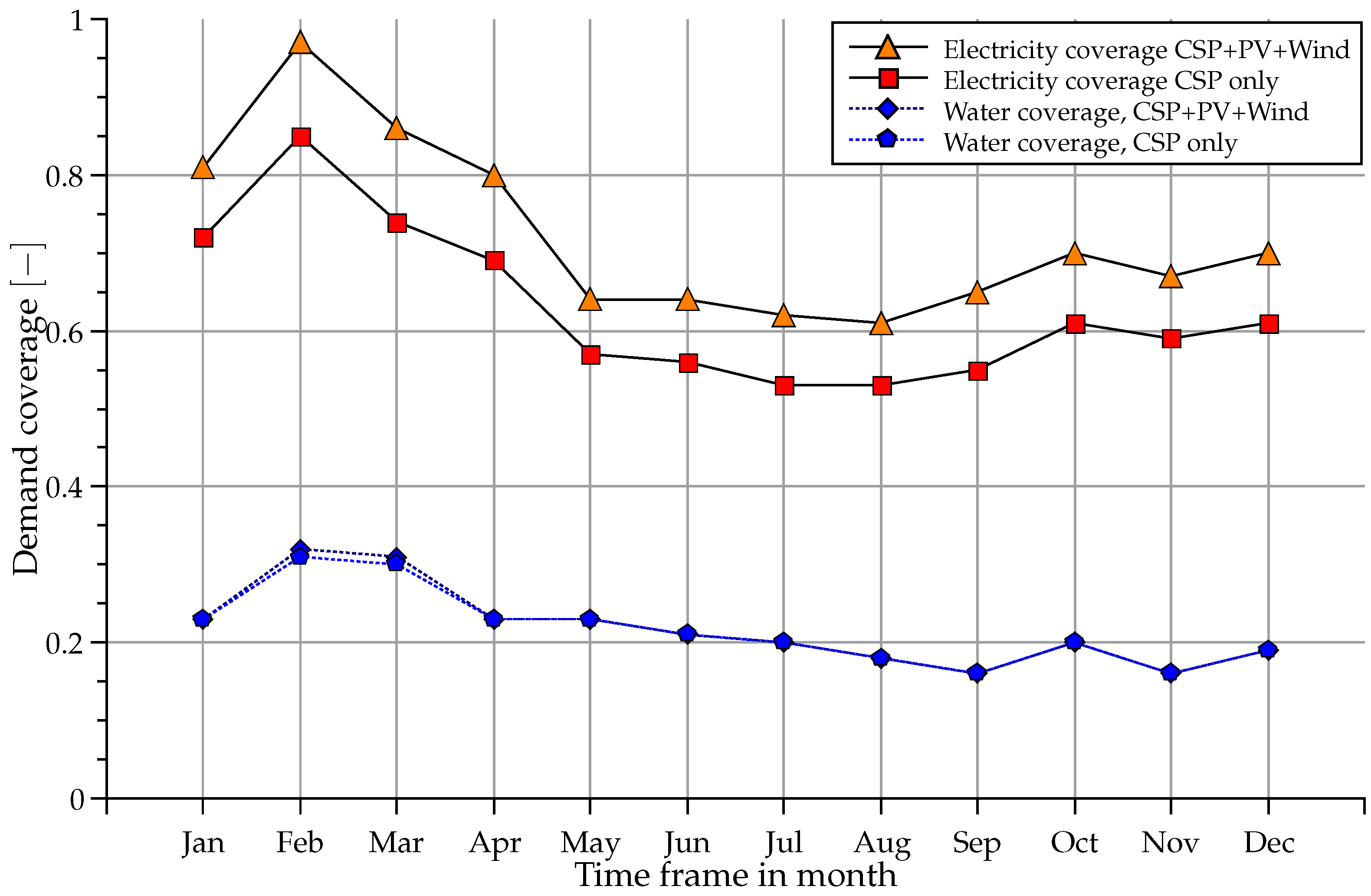
5.4. Total Demand Coverage

The percentages of demand coverage are presented in Figure 9 based on the scaled demand calculated according to Section 3.1. While the total demand coverage of the single CSP system ranges from 53% up to 85%, the integrated system with additional PV and wind power can increase the coverage up to 98%. The yearly coverage sums up to 61% using only the CSP plant while the integrated system increases the coverage up to 10 percentage points for the electricity demand.

The effect of the integrated system to the water demand coverage is limited, because there is no additional desalination unit connected to the PV and wind power plant. The only extension can be seen during the winter months by the extension of the CSP operation time using the generated surplus power. As the effect does not exceed 1%, it can be concluded that the additional storage of heat has a negligible influence on the total water demand coverage over the complete year.

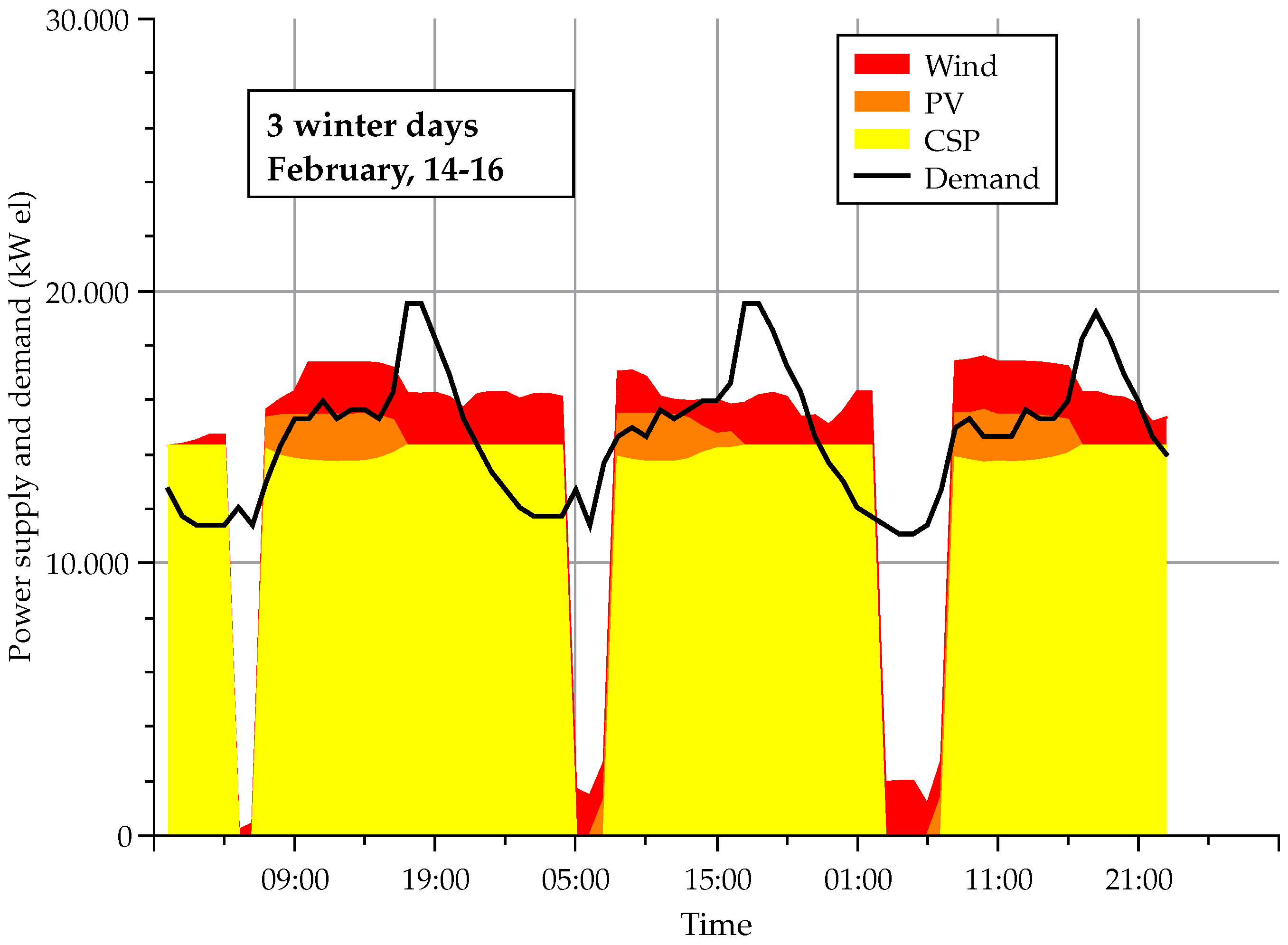
Concerning the electricity demand, the Figure 10 and Figure 11 compare three typical days during the summer and winter seasons. They present the renewable energy mix by the integrated system. Furthermore, the analysis of the winter days in Figure 10 visualize the evolution of surplus power, which is discussed in the following section.

However, Figure 10 and Figure 11 allow a conclusion in terms of residual power demand which needs to be supplied from the national grid. The winter days in Figure 10 show an interrupted operation of the CSP plant during hours with low loads creating gaps of two or three hours down-time. During those hours, the wind power plant decreases the residual power demand depending on the actual wind condition. The strong ascending power demand during the morning hours is supported by the solar energy plants (both PV as well as the CSP). February, 15th, shows a lowered irradiation in the afternoon hours which lowers the PV plant power generation as well as the operation time of the CSP in the following night.

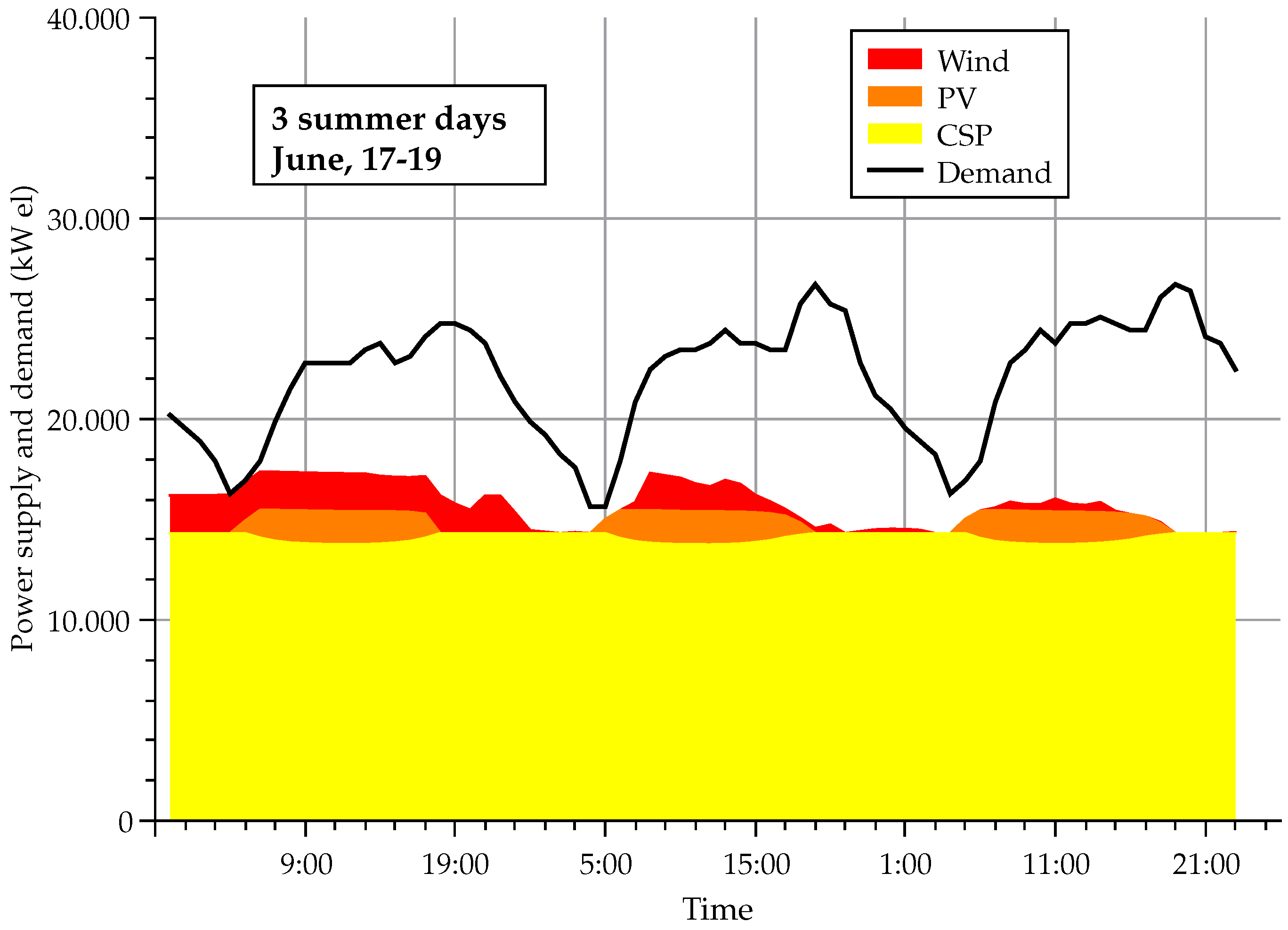
During the summer days (Figure 11), the CSP plant can continuously operate providing firm capacity to the demand. The power generated by the fluctuation resources fit to a certain extend to the needed electricity, but do not cover the peak loads around 7:00 pm. Furthermore, the electricity demand of the molten salt pumps cause a slight decline of the CSP power output of around 600 ${\mathrm{kW}}_{\mathrm{el}}$ during the day. The parasitic energy consumption of the heliostat field and molten salt pumps fit exactly to the generated power of the PV plant. Therefore, the whole integrated system is not influenced by this power decline during day operation. The combination of CSP and PV seems to be beneficial in order to minimize the parasitic losses of the power plant.

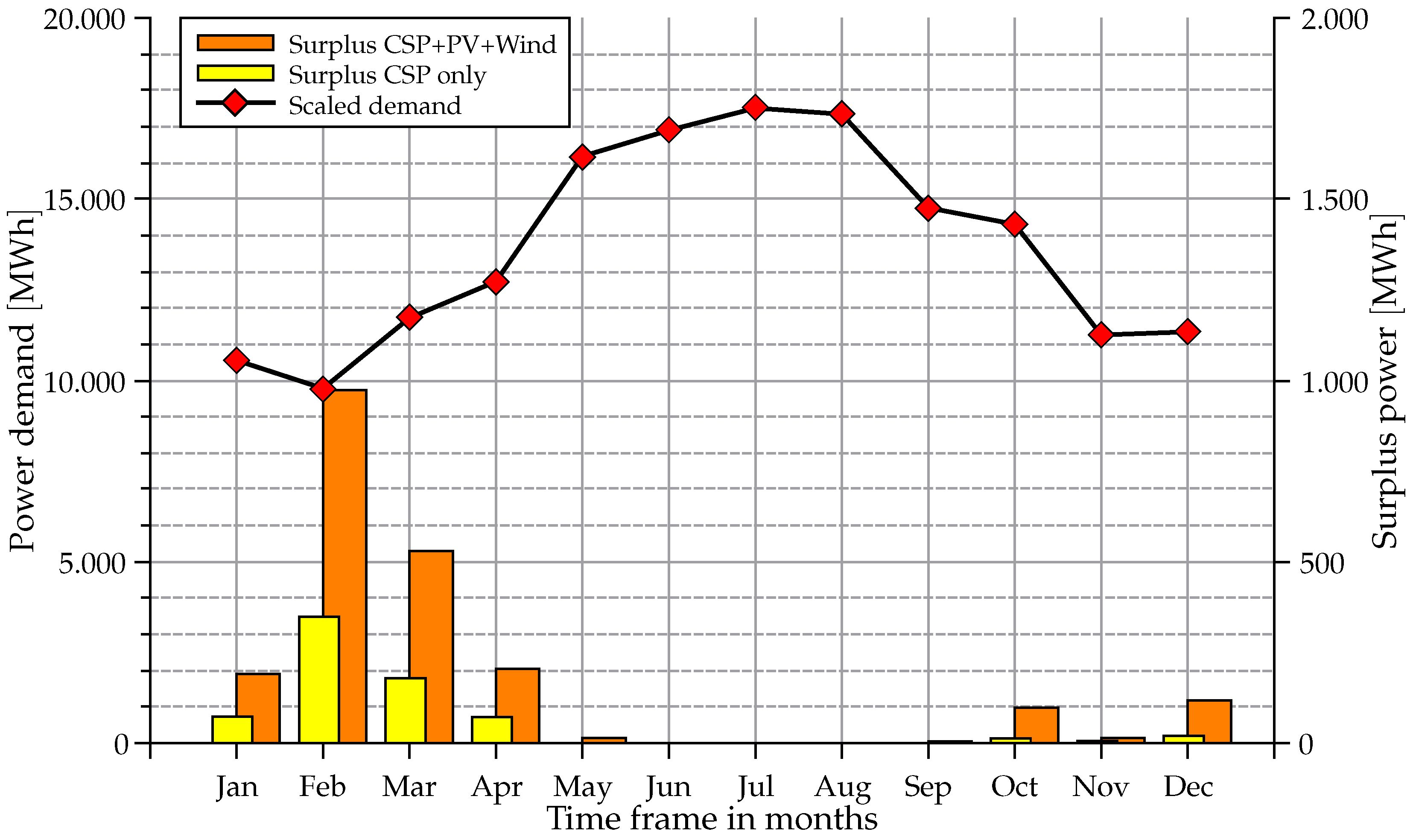
5.5. Generation of Surplus Power

The occurrence of surplus power results when the supply exceeds the actual power demand. Especially when using fluctuating energy sources like PV and wind power it is favored to use the surplus generation, which can be either stored or fed to the grid (compare also to Figure 10).

In the discussed configuration, only the CSP plant allows to deliver power on demand depending on the actual level of the thermal storage system. If the irradiation during the day cannot charge the storage sufficiently, the power generation is reduced because of the empty hot storage tank. The maximized operation of the CSP plant only creates a total cumulative surplus of 711 ${\mathrm{MWh}}_{\mathrm{el}}$ during the year.

Adding the PV and wind power plant with a design capacity of 4 ${\mathrm{MWh}}_{\mathrm{el}}$ doubles the generated surplus power to 1434 ${\mathrm{MWh}}_{\mathrm{el}}$ during the year, generating a total surplus of 2145 ${\mathrm{MWh}}_{\mathrm{el}}$. Figure 12 presents the surplus power by monthly values on the right axis with respect to the scaled power demand. The highest surplus is generated during the months January to April. The peak surplus sums up to 5605 ${\mathrm{kW}}_{\mathrm{el}}$ in February. During the summer term with generally high electricity demand, the generated surplus drops almost to zero. All generated power by the renewable energy system meets the scaled demand and can be used directly.

5.6. Storage of Surplus Power

The whole generated surplus is converted into usable heat for the thermal storage system. As the consequence of that, the process allows the direct utilization of generated power to increase the operation time of the CSP plant. Under the stated assumptions (Section 4), a peak power of 5000 ${\mathrm{kW}}_{\mathrm{el}}$ generates additional 41.8 $\mathrm{t}/\mathrm{h}$ molten salt in the hot storage tank. Comparing the amount to 300 $\mathrm{t}/\mathrm{h}$ mass flow used for steam generation, in the examined case the extension of the additional run-time of the CSP plant is only marginal.

Figure 13 visualizes the increased operation time of the CSP by generated surplus power from the PV and wind power plant. It can be stated that only during the winter is a noticeable extension of the CSP operation time. The CSP power generation is increased by up to 4.5% in February, the other months show a negligible extension of the operation time in the range of 1%–2%. The calculation of the complete year results in a generated power extension of 0.8%.

Table 11. Total power generation, available surplus and additional CSP operation time.

Month	Total Power Generation ${\mathbf{MWh}}_{\mathbf{el}}$	Surplus Generated ${\mathbf{MWh}}_{\mathbf{el}}$	Additional CSP Operation Time $\mathbf{h}$
January	8520	190	6.36
February	9787	978	27.26
March	10037	529	14.75
April	10206	205	5.71
May	10431	13	0.38
June	10866	0	0
July	10866	0	0
August	10568	0	0
September	9544	4	0.12
October	9981	97	2.71
November	7516	14	0.47
December	7956	118	3.95
Total	116,277	2150	61.70

presents the total power generation per month, the generated surplus power and the resulting additional CSP operation time. The highest amounts of surplus power evolves during the winter (Figure 12). The resulting extension of the CSP operation ranges up to 27 h in February and zero during the summer. In total, the yearly extension reaches almost up to 62 h for the complete year.

The reason for the limited effect in this scenario has several causes. First of all, the dimension of the PV and wind power plant is rather small compared to the CSP plant. The design capacity of 4 ${\mathrm{MW}}_{\mathrm{el}}$ for both technologies hold only a minor share compared to the 14 ${\mathrm{MW}}_{\mathrm{el}}$ CSP design capacity. Increasing the amount of PV and wind power installed, would generate higher amounts of surplus energy which can be stored using the thermal storage system of the CSP plant. However, the whole integrated system has been dimensioned in order to generally minimize the generation of surplus power. The goal of this study has been the dimension of a system to cover the demand of the city, not to feed-in power to the national grid. The available land area in coastal regions with seawater access is limited and preferably used for touristic purposes.

5.7. Estimation of Investment Cost

In order to estimate the capital investment for the integrated energy supply system, the results from Section 5.3 are used. All values have been calculated using SAM [21]. The total investment costs (total CAPEX) for the complete integrated system sum up to 154.2 $\mathrm{mil}\$$ at a total power generation of 115.3 ${\mathrm{GWh}}_{\mathrm{el}}$. More than 80% of the total CAPEX can be accounted to the CSP plant with the thermal storage system. The reasons are the high costs of the heliostat field, the receiver and the tower itself, which need to be dimensioned according to the storage system. The desalination unit shares only around 2% due to the replacement of the power plant cooling system.

Basing on the monthly power generation of each technology and the weighed averaged mean share of the electricity supply, the derivation of a common $LCO{E}_{tot}$ value of the integrated system becomes possible.

Table 12. Integrated system, total levelized cost of electricity.

Technology	Total Power Generation ${\mathbf{MWh}}_{\mathbf{el}}$	Levelized Cost ct/$\mathbf{kWh}$	Averaged LCOE ct/$\mathbf{kWh}$
CSP	100,978	18	15.7
PV	5948	21	10.8
Wind	8327	1	0.01

summarizes the calculation for the discussed system configuration. Due to the technology characteristics and the complexity of the integrated system, a more detailed investigation and optimized plant sizing could be subject to further research.

The lower investment cost and economic performance of wind model plant decrease the $LCO{E}_{CSP}$ by 2.3 $\mathrm{ct}/\mathrm{kWh}$ and the $LCO{E}_{PV}$ by 10 $\mathrm{ct}/\mathrm{kWh}$. The effect is caused by the wind power plant which generates a financial benefit due to the excellent wind conditions at the selected site (measurement base on [5]). The total levelized costs of electricity $LCO{E}_{tot}$ calculate to 17 ct$/\mathrm{kWh}$ without any governmental incentives or subsidies. Furthermore, it needs to be noted that the deployment of wind power plants appears to be financially more profitable compared to solar energy systems.

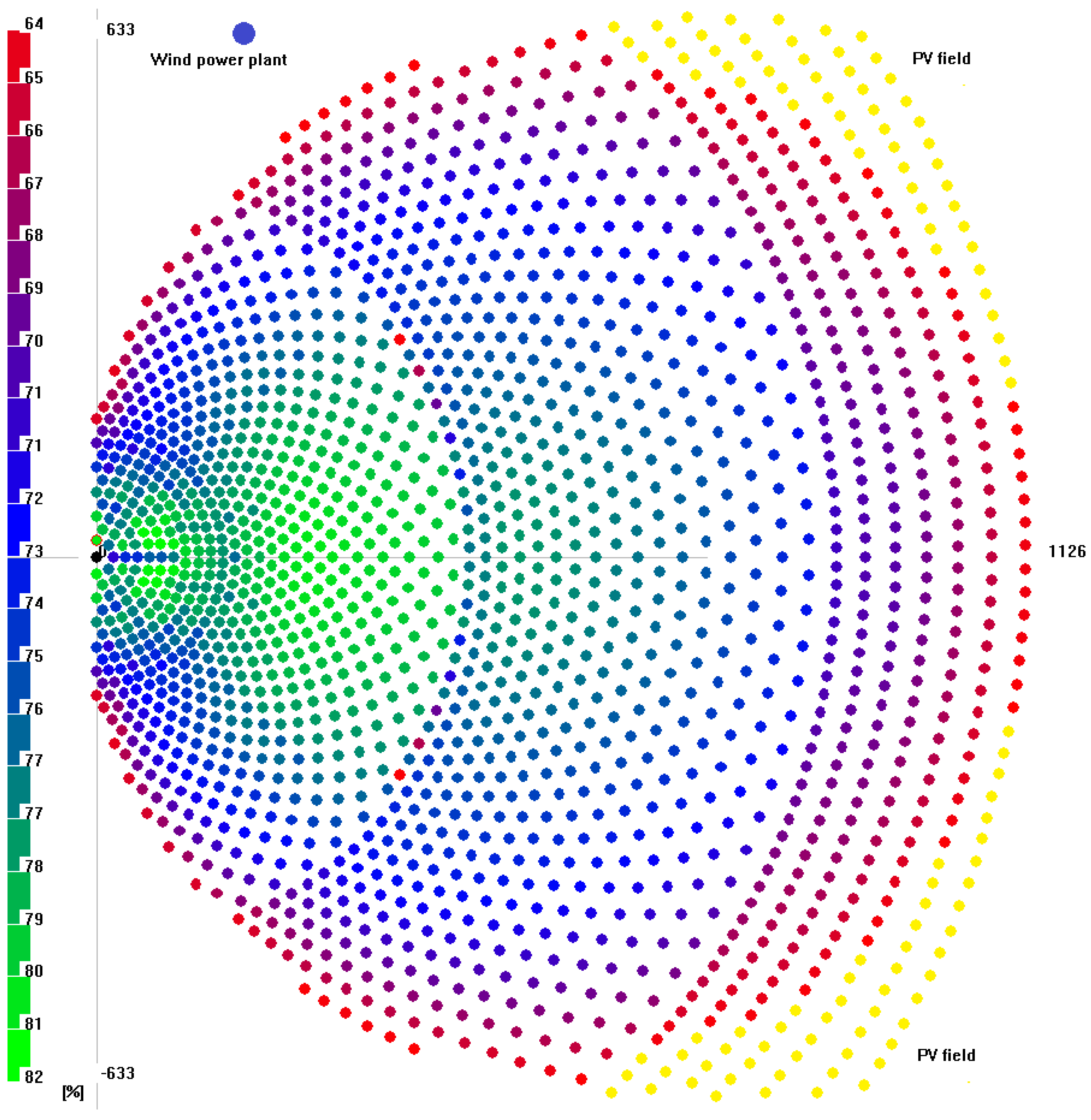
5.8. Integration and Occupied Land Area

Due to the arrangement of the heliostats around the tower (Figure 14), the occupied land principally has a round shape. Based on the assumptions (Section 3.3), the integrated power supply system is integrated in the given layout of the field. The assembly of PV modules on given heliostats replacing the mirrors lead to cost advantages through economies of scale. In addition, the PV modules generate more electricity by orientating them continually in an optimal angle to the solar irradiation.

The wind turbine can be placed optionally on the edges of the field. The analysis of the meteorological data has shown that the most frequent wind direction is North-West. As a result, one possible option to integrate the PV and wind model plant given in Figure 14. The total occupied land area calculates to 1266 × 1126 $\mathrm{m}$, which sums up to an total area of 1.426 ${\mathrm{km}}^2$.

The required land is marked in Figure 15. The locations is chosen close to the road Hurghada—Cairo in order to allow a possible expansion of the city on undeveloped land. The presence of an own substation connected to the national grid as well as a waste-water treatment plant simplifies the media connection for electricity and water.

The position of each heliostat is subject to further optimizations in order to respect the land surface and the field efficiency. It is required to respect possible elevations and ground conditions as well as the distance to the seawater source. As a consequence, Figure 15 presents just one possible solution according to the performed simulation of the solar power plant.

6. Conclusions

The paper presented an energy and water supply system which has been integrated into a real scenario using an energy mix of CSP, PV and wind power plants based on a given demand scenario. The technological approach to combine these processes takes the different power generation characteristics into account. Furthermore, the process integration has also some general advantages like lowering the dependencies on fossil fuels, a consequent reduction of climate gas emissions, and the protection of finite water reserves. However, the economic assessment pointed out that the approach is significantly more costly compared to conventional power solutions with respect to the current subsidization of fossil energy carriers.

The main reason for the high costs can be accounted to the CSP system with the integrated thermal desalination unit, which account for more than 80% to the total installation costs. The impact of the new developed low-temperature desalination is only marginal because the installation costs range around 2% of the total system costs. The main costs drivers are the heliostat field, the tower and the receiver. Those components need to be designed with respect to the large thermal storage system and create additional costs.

The short-term storage of surplus energy by thermal processes need a special investigation on the level of technical solutions and respective plant components. In the specific case, the solution does not seem advantageous due to the minor occurrence of surplus power which should be fed into the electricity grid. The economic benefits may increase with the amount of variable renewable power supply systems, demanding for simple storage solutions with insensitive part-load behavior and short ramp-up times. Other approaches like smart-grids and energy price changes may result in different conclusions who can make the proposed system financially more advantageous than previously described.

Due to the special construction and operation of the CSP plant, there are also other options for the integration of the co-generation products technically feasible which have not been discussed. The avoidance of surplus power generation could be performed basing on flexible condensation pressures in order to increase to the water production when the electricity demand is low. This requires a detailed optimization of the CSP power generation with respect to the fluctuating resources like the modeled PV and wind power plant. The water production can be maximized when the power demand is minimized in order to cover the demand more precisely. The influence of changed boundary conditions and financial assumptions can have a significant effect on the results and will be subject of further research.

References

- Birol, F.; Cozzi, L.; Gül, T.; Dorner, D.; Baroni, M.; Besson, C.; Hood, C.; Wanner, B.; Wilkinson, D. World Energy Outlook: Redrawing the Energy-Climate Map; Technical Report; International Energy Agency (IEA): Paris, France, 2013. [Google Scholar]
- Birol, F.; Cozzi, L.; Gould, T.; Bromhead, A.; Gül, T.; Frank, M. World Energy Outlook; Technical Report; International Energy Agency (IEA): Paris, France, 2012. [Google Scholar]
- Wellmann, J.; Neuhäuser, K.; Behrendt, F.; Lehmann, M. Modeling the cogeneration of power and water with csp and low temperature desalination. In Proceedings of the 3rd Desert Energy Conference, Berlin, Germany, 7–8 November 2012.
- Wellmann, J.; Neuhäuser, K.; Behrendt, F.; Lehmann, M. Modeling an innovative low-temperature desalination system with integrated cogeneration in a concentrating solar power plant. Desalination Water Treat. 2014, 55, 1–9. [Google Scholar] [CrossRef]
- Wellmann, J.; Langer, I. Weather Station el Gouna West, Measurement Data of 2013; Geographic coordinates: Lat. 27.412906 Long. E 33.638252, TU Berlin, Campus El Gouna and FU Berlin, Institut für Meteorologie; TU Berlin, Department Energy Engineering: Berlin, Germany, 2013. [Google Scholar]
- Tzoupanos, N.; Estafanous, S. Drinking Water Consumption of el Gouna, Red Sea, Egypt; TU Berlin, Campus El Gouna 2014; Department Water Engineering and El Gouna Water: El Gouna, Egypt, 2014. [Google Scholar]
- Estafanous, S. El Gouna Power and Water Supply; Orascom Hotels and Development, El Gouna Electrics: El Gouna, Egypt, 2015. [Google Scholar]
- Cole, G. El Gouna Goes Carbon Neutral; Sawiris Foundation for Environmental Development: Cairo, Egypt, 2014. [Google Scholar]
- Remund, J.; Müller, S.; Kunz, S.; Huguenin-Landl, B.; Studer, C.; Klauser, D.; Schilter, C. Meteonorm, Global Meteorological Database; Handbook Part I, Software, 7.1 ed.; Meteotest: Bern, Switzerland, 2014. [Google Scholar]
- Remund, J.; Müller, S.; Kunz, S.; Huguenin-Landl, B.; Studer, C.; Klauser, D.; Schilter, C. Meteonorm, Global Meteorological Database; Handbook Part II, Theory, 7.0.0 ed.; Meteotest: Bern, Switzerland, 2012. [Google Scholar]
- Tzoupanos, N. Water and Wastewater Management in El Gouna, Red Sea, Egypt; TU Berlin Campus El Gouna, Department Water Engineering: Berlin, Germany, 2015. [Google Scholar]
- Azzer, T.; Rizkalla, E.; Naseem, H. Electricity Demand of el Gouna 2013; Time Series of Electricity Demand in hourly values (unpublished); 2014. [Google Scholar]
- Egyptian Electricity Holding Company (EEHC). Annual Report 2012/13; Technical Report; Egyptian Electriciy Holding Company: Cairo, Egypt, 2013. [Google Scholar]
- STEAG Energy Services GmbH. EBSILON Professional Documentation; STEAG Energy Services GmbH: Zwingenberg, Germany, 2012. [Google Scholar]
- Marto, P.J. Condensation. In McGraw-Hill Handbooks, 3rd ed.; McGraw-Hill: New York, NY, USA, 1998. [Google Scholar]
- Lehmann, M.; Exer, G.; Merkli, C. Low Temperature Distillation System by Watersolutions (WS-LTD); General Plant and Process Description; Water Solutions AG: Buchs, Switzerland, 2012. [Google Scholar]
- Lehmann, M. Grundlagen zur Simulation des WS-Ltd Niedertemperatur Entsalzungsmodul für Variable Temperaturspektren und Variable Stufigkeit; Unpublished Internal Paper; Watersolutions AG: Buchs, Switzerland, 2012. [Google Scholar]
- Loveday, T. Is low temperature the next hot prospect? Desalination Water Treat. 2015, 24, 23–25. [Google Scholar]
- Mansfeldt, E.; Lehmann, M.; Exer, G.; Merkli, C. Process Comparison MED/WS-LTD; (unpublished); Watersolutions AG: Buchs, Switzerland, 2013. [Google Scholar]
- Neuhäuser, K. Modellierung Einer Niedertemperatur Entsalzungsanlage mit Integration in ein Solarthermisches Kraftwerk. Master’s Thesis, Institut für Energietechnik, Berlin, Germany, 2013. [Google Scholar]
- Blair, N.; Dobos, A.P.; Freeman, J.; Neises, T.; Wagner, M.; Ferguson, T.; Gilman, P.; Janzou, S. System Advisor Model (SAM) General Description; Technical Report NREL/TP-6A20-61019; National Renewable Energy Laboratory: Golden, CO, USA, 2014.
- Trieb, F. Pv performance model. In Proceedings of the Script for the Lecture Integration of Renewable Energies, Campus El Gouna, Egypt, November 2012. Section 11.
- Normenausschuss Lichttechnik (FNL) (Ed.) DIN 5035: Tageslicht in Innenräumen; Deutsches Institut für Normung e.V. (DIN): Berlin, Germany, 1985.
- Bosch Solar Energy AG. Bosch solar module c-Si M 60 s; M245, 245 wp; BOSCH Solar Energy AG: Erfurt, Germany, 2013. [Google Scholar]
- Trieb, F. Wind performance model. In Proceedings of the Script for the Lecture Integration of Renewable Energies, El Gouna, Egypt, November 2012. Section 12.
- ENERCON. Enercon Produktübersicht; Technical report; ENERCON GmbH: Aurich, Germany, March 2014. [Google Scholar]
- Reddy, R.G. Novel Molten Salts Thermal Energy Storage for Concentrating Solar Power Generation; Presentation, Solar Energy Technologies Program Peer Review; US Department of Energy: Washington, DC, USA, 2010.
- Bauer, T.; Pfleger, N.; Breidenbach, N.; Eck, M.; Laing, D.; Kaesche, S. Material aspects of solar salt for sensible heat storage. Appl. Energy 2013, 111, 1114–1119. [Google Scholar] [CrossRef]
- Mauleón, I. The cost of renewable power: A survey of recent estimates. In Green Energy and Efficiency; Ansuategi, A., Delgado, J., Galarraga, I., Eds.; Green Energy and Technology; Springer International Publishing: Cham, Switzerland, 2015; pp. 235–268. [Google Scholar]
- AT Kerney GmbH. Solar Thermal Electricity 2025–Clean Electricity on Demand: Attractive STE Cost Stabilize Energy Production; Technical Report; European Solar Thermal Electricity Association: Brussels, Belgium, 2010; AT Kearney GmbH. [Google Scholar]
- Moser, M.; Trieb, F.; Fichter, T.; Kern, J.; Hess, D. A flexible techno-economic model for the assessment of desalination plants driven by renewable energies. Desalination Water Treat. 2015, 55, 3091–3105. [Google Scholar] [CrossRef]
- Negewo, B.D. Renewable Energy Desalination: An Emerging Solution to Close the Water Gap in the Middle East and North Africa; The World Bank: Washington, DC, USA, 2012. [Google Scholar]
- Kulichenko, N.; Wirth, J. Concentrating Solar Power in Developing Countries: Regulatory and Financial Incentives for Scaling Up; The World Bank: Washington, DC, USA, 2012. [Google Scholar]
- Turchi, C.; Heath, G. Molten Salt Power Tower Cost Model for the System Advisor Model; Technical Report No. NREL/TP-5500-57625; National Renewable Energy Laboratory: Golden, CO, USA, 2013.
- Valero, A.A.; Serra, L.L.; Uche, J.J. Fundamentals of exergy cost accounting and thermoeconomics. Part I: Theory. J. Energy Resour. Technol. 2005, 128, 1–8. [Google Scholar] [CrossRef]
- Sommariva, C. Desalination and Advanced Water Treatment: Economics and Financing; Balaban Desalination Publications: Rome, Italy, 2010. [Google Scholar]
- Li, K.W. Applied Thermodynamics: Availability Method And Energy Conversion; Taylor & Francis: Philadelphia, PA, USA, 1995. [Google Scholar]
- Wade, N.M. Energy and cost allocation in dual-purpose power and desalination plants. Desalination 1999, 123, 115–125, presented at The {WSTA} Fourth Gulf Water Conference. [Google Scholar] [CrossRef]
- IRENA. Renewable Energy Technologies, Cost Analysis Series: Concentrating Solar Power. Volume 1: Power Sector, Issue 2/5; International Renewable Energy Agency (IRENA): Bonn, Germany, 2012. [Google Scholar]
- International Renewable Energy Agency (IRENA). Renewable Energy Technologies, Cost Analysis Series: Solar Photovoltaics. Volume 1: Power Sector, Issue 4/5; International Renewable Energy Agency (IRENA): Bonn, Germany, 2012. [Google Scholar]
- Kost, C.; Mayer, J.N.; Thomsen, J.; Harmann, N.; Senkpiel, C.; Philipps, S.; Nold, S.; Lude, S.; Schlegl, T. Stromgestehungskosten Erneuerbare Energien; Technical Report; Fraunhofer-Institut für Solare Energiesysteme (ISE): Freiburg, Germany, 2013. [Google Scholar]
- US Energy Information Administration (EIA). Updated Capital Cost Estimates for Utility Scale Electricity Generating Plants; US Energy Information Administration (EIA): Washington, DC, USA, 2013.
- Windpark Maierfeld in den Marktgemeinden Kindingen und Titting. Strom aus Wind—Eine Investition in Unsere Zukunft; Technical Report; Beermann Windkraft GmbH: Maierfeld, Germany, 2011. [Google Scholar]
- International Renewable Energy Agency (IRENA). Renewable Power Generation Costs in 2012: An Overview; Technical Report; International Renewable Energy Agency (IRENA): Bonn, Germany, 2013. [Google Scholar]
- Krohn, S.; Morthorst, P.E.; Awerbuch, S. The Economics of Wind Energy; Report; European Wind Energy Association: Brussels, Belgium, 2009. [Google Scholar]
- Bürgerinitiative für einen verantwortungsvollen Umgang mit Windenergie. Wirtschaftlichkeit der WKA in Gailingen; Technical Report; 2012; Available online: http://gegenwind-husarenhof.de/sonstiges/Wirtschaftlichkeit%2520der%2520WKA%2520in%2520Gailingen_April_2012_sec.pdf (accessed on 29 March 2016).
- Schwarzbözl, P.; Pitz-Paal, R.; Belhomme, B.; Schmitz, M. Visual-hflcal—Eine Software zur Auslegung und Optimierung von Solarturmsystemen; Deutsches Zentrum für Luft- und Raumfahrt (DLR): Cologne, Germany, 2011. [Google Scholar]
- Schwarzbözl, P.; Belhomme, B.; Buck, R.; Uhlig, R.; Amsbeck, L.; Schmitz, M. Simulation Solar Turmsysteme; Deutsches Zentrum für Luft- und Raumfahrt (DLR): Cologne, Germany, 2012. [Google Scholar]
© 2016 by the authors; licensee MDPI, Basel, Switzerland. This article is an open access article distributed under the terms and conditions of the Creative Commons by Attribution (CC-BY) license (http://creativecommons.org/licenses/by/4.0/).