Characterizing and Assessing the Agricultural Land Use Intensity of the Beijing Mountainous Region

Abstract

Recently, land use and land cover change have received increased attention, and an approach is required that can assess agricultural land use intensity on a general basis. This study demonstrated the usefulness of a tool for characterizing and assessing agricultural land use intensity in Beijing mountainous region. An emergy analysis and principal component analysis (PCA) were adopted to obtain agricultural input and output intensity data. Correlation and regression analyses were used to study the relationship among land capability, agricultural input, output intensity, and agricultural system sustainability. Ultimately, the agricultural land use intensity types in the Beijing mountainous region were identified through a cluster analysis. The results produced five indices of agricultural input intensity and five indices of output intensity. Non-renewable energy was the overwhelming input, and grain, meat, eggs, and vegetables were the major outputs of the agricultural system. The results also showed that there was better natural land quality, higher input intensity, greater output intensity, and lower agricultural system sustainability. Eight types of agricultural intensity were classified and assessed, and they may be used to evaluate and monitor sustainable land use and provide baseline measurements of land use intensity for land use analyses and change detection.

1. Introduction

Land use and land cover change has affected the structure and function of ecosystems in different ways [1] and is central to the sustainable development debate [2]. Whilst most previous land use and land cover change research was focused on land cover conversions, such as deforestation and urbanization, more subtle processes leading to a modification of land cover deserves more attention. In the research of land use and land cover change, land cover conversion is defined as the complete replacement of one cover type by another, and land cover modification is referred to as more subtle changes that affect the character of the land cover without changing its overall classification [3]. Land cover modification is frequently caused by changes in the management of agricultural land use including, e.g., changes in levels of inputs and the effect of this on profitability, or the periodicity of complex land use trajectories, e.g., fallow cycles, rotation systems, or secondary forest regrowth [2].

As the population grows and dietary habits change, future demand for agricultural products will increase over the coming decades. The two basic options for this are the expansion of the land area under agricultural production, and increases of output per unit area in agriculture. Most of the related growth in agricultural production will have to rely on increases of output per unit area in agriculture rather than on the limited land expansion. Such increased output on currently used land is commonly described by the broadly accepted, but ambiguously defined, notion of ‘land use intensification’. In addition, land use intensity is the degree of yield amplification, which is related to changes in levels of inputs and outputs. When land use intensity changes, land cover modification occurs. Land use intensification is one of the most significant forms of land cover modification, with dramatic increases in agricultural production being the main feature. With the increased attention to processes of land cover modification, we should especially pay more attention to land use intensification and intensity. Land use intensification and intensity research would be helpful for providing a better understanding of the complex relationships between people and land resources management, and additional sustainable land resource maintenance.

Beginning at least with von Thünen in 1842, agricultural intensity (viewed in terms of production or yield per unit area and time) has long been regarded as a key concept in numerous explanations of agricultural growth and change [3]. Until now, many researchers have defined and quantified the terms ‘land-use intensification’ and ‘land use intensity’. The concept of intensification in land use often, although not exclusively, refers to agriculture. Brookfield [4] describes intensification as being ‘in relation to constant land, the substitution of labor, capital or technology for land, in any combination, so as to obtain higher long-term production from the same area’. Kates et al. [5] and Netting [6] use the formulation that intensification is ‘a process of increasing the utilization or productivity of land currently under production, and it contrasts with expansion, that is, the extension of land under cultivation’. Shriar [7] uses the formulation that ‘agricultural intensification is a process of raising land productivity over time through increases in inputs of one form or another on a per unit area basis’ and measures agricultural intensity based on agrotechnologies, practices, and their degrees of use by farmers by assigning a weight to each input activity with some subjectivity. Kerr and Cihlar [8] used a principal components analysis (PCA) to integrate the major material inputs and by-product outputs for measuring land use intensity to assess the potential for pollution in agricultural areas. Herzog et al. [9] proposed intensity indicators of fertilizer input, livestock density, and pesticide input that affect the environment in terms of biodiversity and water quality, and developed an overall intensity index by normalizing the selected intensity indicators to explain land use intensity at the landscape level. Research over the last decade has used material flow and input-output to assess the environmental impacts of systems, products, and services, as well as land use systems [10,11]; for example, human appropriation of net primary production (HANPP) was used as the indicator of land use intensity to measure the pressure of human use of land in a defined territory by Wrbka et al. [12]. In China, the study of land use intensity has been relatively simple and has primarily expressed regional land use intensity based on the characteristics of various land use types, without considering input or output [13,14].

Currently, the description of land use intensification/intensity is diverse, and is associated with a lack of measurable criteria. Comparing all of these definitions and measures, we find that intensification/intensity is mostly measured by purchased economic inputs, such as labor, fertilizers, pesticides, mechanical equipment, and some other industrial products. Changes in productivity due to environmental inputs, such as sunlight, rain, and soil, are generally excluded. Agriculture operates at the interface between nature and human economy and combines natural resources and economic inputs to produce food [15]. Intensive agricultural methods reply more on resources purchased from the economy, while less intensive and indigenous methods typically reply more on natural inputs. Hence, considering natural and economic inputs and agricultural outputs together as intensity indices can provide a holistic measure of agricultural land use intensity. Such an approach is also helpful in understanding the relationship between the inputs and outputs regarding the sustainability of an agricultural system.

Since most types of agriculture depend on a combination of natural and economic inputs, it is necessary to account for both in equivalent terms when comparing the agricultural resource use and further characterizing agricultural land use intensity. Emergy analysis, which evaluates system components on a common basis, is a promising tool to evaluate agricultural resource use and production. The emergy, which was proposed by Odum for system analysis, accounting, and diagnosis, was defined as the available energy of one kind previously used up directly and indirectly to make a service or product, usually quantified in solar energy equivalents and expressed as solar emJoules (sej) [16]. The ratio of emergy required to make a product or service is defined as the tansformity, and the corresponding solar emjoules emergy of a product or service is calculated by multiplying units of energy by transformity. Using this technique, natural and economic contributions required to produce agricultural yields can be quantified and compared on a common basis of solar emergy-joules. Emergy analysis has been used to evaluate the sustainability of agricultural methods in Australia, Sweden, Italy, Thailand, and China, etc.

Additionally, more work is needed to assess the agricultural land use intensity effect on the sustainability of an agricultural system. From a sustainability point of view, the agricultural land use intensity should match land quality with there being a high ratio of output to input, minimal imports, and minimal environmental load. A land capability classification system was established by the Soil Conservation Service of the United States of America that is general, simple, and easy to understand. It has, thus, been widely used throughout the world for land quality evaluations. There are eight classes designated by roman numerals, from I–VIII. Increasing class number indicates a lower capability, and the classes indicate the location, amount, and general suitability of soils for agricultural use and the risk of land degradation. In relation to an agro-ecosystem, an emergy sustainability index (ESI), as one of emergy indices, was developed by Ulgiati et al. [17], Brown and Ulgiati [18], and Ulgiati and Brown [19], and the ESI considers both ecological and economic compatibility [20]. As pointed out by Ulgiati and Brown [19], a higher index means that an economy is more reliant on renewable energy sources and minimizes imports and environmental load.

The agricultural system in Beijing has played an increasingly important role in areas such as services, the economy, ecology, and tourism, because of the population increase and urban sprawl of Beijing. However, environmental damage caused by agriculture, especially high-intensity industrialized agriculture, has greatly increased. Moreover, land use changes in the Beijing mountainous region have caused many land-related problems, such as water pollution, soil contamination, and air pollution [21], and reduced the productivity and sustainability of agricultural systems. It is important to derive suitable land use intensity “thresholds” as guidelines for planners and managers to reconcile agricultural and environmental economic objectives. Hence, an improved understanding of land use intensity characteristics and their relationship with socio-economic conditions in the Beijing mountainous region is vital for Beijing’s sustainable development. However, few studies have quantitatively evaluated the land use intensity of the Beijing mountainous region. This paper seeks to develop a statistical index of land use intensity for the Beijing mountainous region and improve the understanding of the area’s structures for land use monitoring and classification.

The objective of this study is to measure agricultural land use intensity in the Beijing mountainous region while considering the input and output of an agricultural system, and to assess the relationship of agricultural land use intensity, land capability, and an emergy sustainability index indicating the effect on the sustainability of an agriculture system.

2. Materials and Methods

2.1. Study Areas

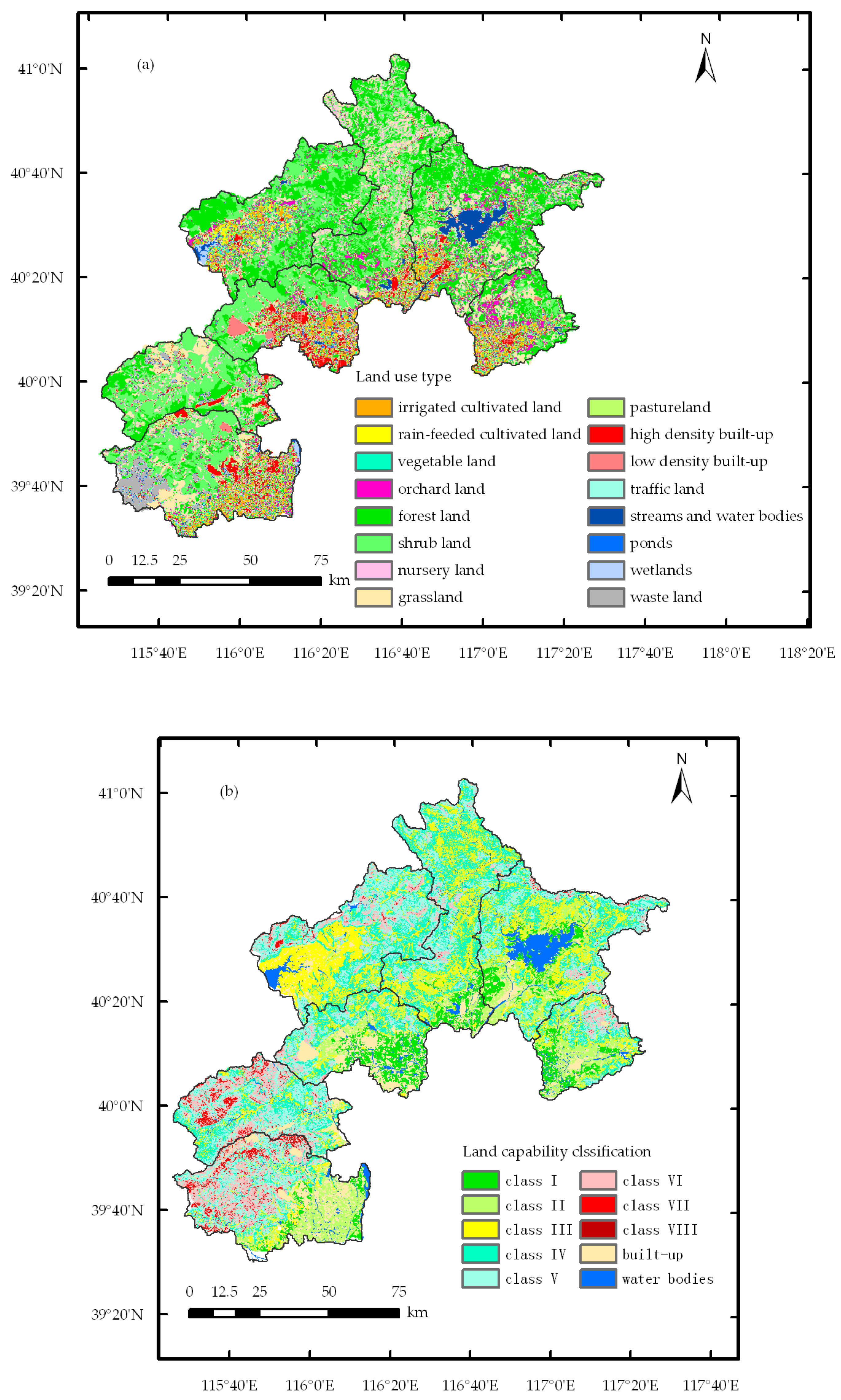
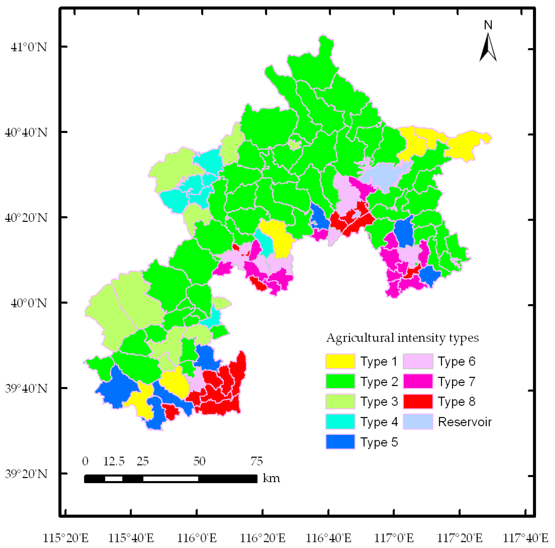
The Beijing mountains region is between 115°24′ and 117°30′E longitude and 39°38′ and 41°05′N latitude and located in the west, north, and northeast of Beijing. There are five suburban districts and two counties, which contain 112 towns, and they account for 62% of the municipal total area (Figure 1). The elevation within the mountain zone ranges from 80–2303 m above mean sea level, and nearly half the area has slopes greater than 15°. The area has a temperate continental monsoonal climate with an annual average temperature of 11.8 °C (average maximum 26 °C in July and average minimum −5 °C in January). The annual average temperature difference is 30.4 °C, and the daily average temperature difference is 11.4 °C. Temperatures change significantly with elevation in the region, decreasing on an average by 0.6 °C per 100 m rise in elevation. The mean annual precipitation in the area is approximately 566 mm, approximately 60% of which is in July and August. The annual average evaporation is approximately 1761 mm. The area is the source of five large rivers, the Yongding, Chaobai, Beiyun, Jiyun, and Daqing. The annual average runoff is approximately 1.8 × 10⁹ m³ but this has decreased to 1.3 × 10⁹ m³ at the end of the last century as a result of climate and land use/cover changes [22].

2.2. Emergy Analysis

Each kind of available energy has its emergy with different units expressed, for example, solar emjoule, coal emjoule, electrical emjoule. Actually, the biosphere is usually considered driven by solar energy and most kinds of available energy are derived from solar energy directly or indirectly. Therefore, solar insolation emergy is used as a common measure in most applications. The solar emergy of products and services is calculated by multiplying units of energy by emergy per energy ratios (transformities), units of mass (i.e., grams of corn) by emergy per mass ratios (specific emergy), and dollars by emergy per unit money. During the past four decades, Odum and his collaborators have calculated transformities for various products and services. There are detailed references for emergy algebra and evaluation [16,17,18,19].

In emergy analysis, inputs to the agro-ecosystem might be categorized into four types: free renewable local resources (RR), such as sunlight, rain, and wind; free non-renewable local resources (NR), soil erosion, for instance; non-renewable purchased industrial subsidiary inputs (NP), such as purchased chemical fertilizers and electricity; and renewable purchased organic inputs (RP), such as labor and oganic manure. Yields of agriculture productions (Y) mainly include the outputs of farming, husbandry, fishery, and forestry, such as crops, vegetables, fruits, meats, forest logging, etc. As most of the agriculture productions are harvested annually, one year is reasonably taken as the time cycle for the agricultural system emergy analysis.

According to the view of emergy analysis, we selected fourteen and twelve variables to characterize agricultural input and output in the Beijing mountainous area (

Table 1. Major agricultural emergy inputs and outputs in the study area.

Number	Item	Transformity (Sej/Unit)	Number	Item	Transformity (Sej/Unit)
Free renewable resources (RR)			Outputs (Y)
1	Sunlight (J)	1.00 × 100	15	Grain crops
2	Rain chemical energy (J)	1.76 × 104	15(1)	Wheat (J)	6.80 × 104
Free non-renewable resources (NR)			15(2)	Corn (J)	2.70 × 104
3	Soil loss (J)	1.92 × 105	15(3)	Millet (J)	3.59 × 104
Non-renewable purchases (NP)			15(4)	Sorghum (J)	8.30 × 104
4	Nitrogen fertilizer (g)	2.41 × 1010	15(5)	Rice (J)	3.59 × 104
5	Phosphorus fertilizer (g)	2.20 × 1010	15(6)	Sweet potato (J)	2.70 × 103
6	Potash fertilizer (g)	1.74 × 109	16	Oil crops (J)	8.60 × 104
7	Compound fertilizer(g)	2.80 × 109	17	Vegetables (J)	2.70 × 104
8	Pesticides (g)	1.48 × 1010	18	Fruits (J)	5.30 × 104
9	Plastic mulch (g)	3.20 × 109	19	Pork (J)	1.70 × 106
10	Mechanized power (J)	5.33 × 104	20	Beef (J)	4.00 × 106
11	Electricity use (J)	2.69 × 105	21	Mutton (J)	2.00 × 106
Renewable purchases (RP)			22	Fowl (J)	1.70 × 106
12	Human labor (J)	3.80 × 105	23	Milks (J)	2.00 × 106
13	Organic manure (J)	9.25 × 104	24	Eggs (J)	4.40 × 106
14	Seed (J)	7.86 × 104	25	Fish (J)	2.00 × 106
			26	Forest logging (J)	4.40 × 104

Transformity references for respective row number: 1. [24]; 2. [24]; 3. [25]; 4. [26]; 5. [26]; 6. [26]; 7. [26]; 8. [26]; 9. [27]; 10. [26]; 11. [24]; 12. [26]; 13. [24]; 14. [24]; 15–26. [26].

), respectively. The analysis was performed on the town scale because the agricultural input and output information derived from census data are aggregated and officially reported at this scale, and the town is also the smallest administrative unit for planning and management purpose in China. Based on the town scale, the analysis results would better link with policies and their assessment. The agricultural input and output data for 112 towns in the year of 2013 were derived from the Statistical Yearbook of five districts and two counties [23]. After quantifying annual inputs and outputs for every town in raw units (joules, grams), these values were multiplied by their respective transformities to calculate the quantity of solar emergy required for each agricultural input and output. The used transformities and their reference sources are listed in Table 1. To make these towns easily comparable, the solar emergy of each agricultural input and output were normalized for agricultural land area, and these values were quantified in solar emjoules per hectare (sej·ha⁻¹).

2.3. Agriculture Input and Output Intensity Indices (In and Out)

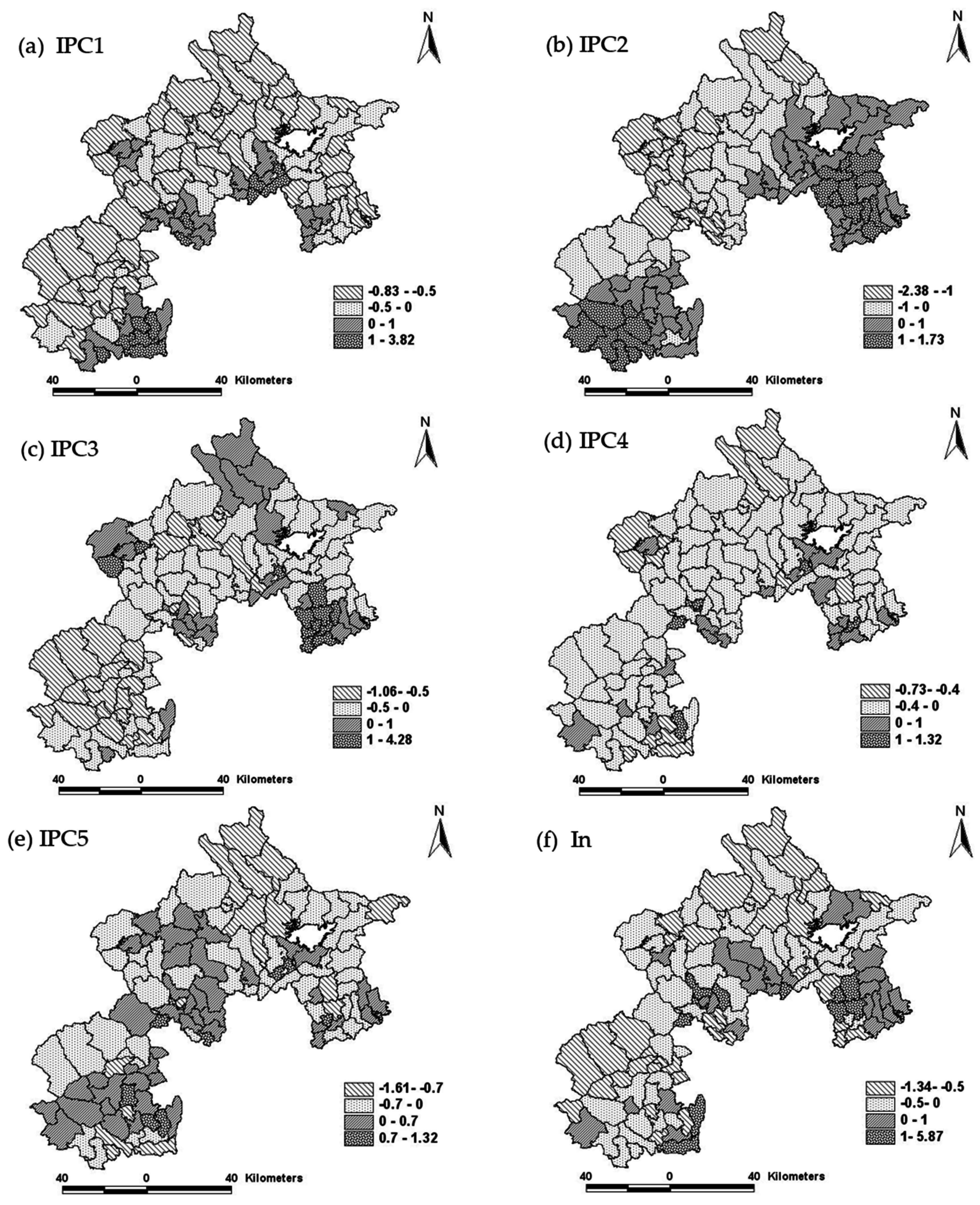
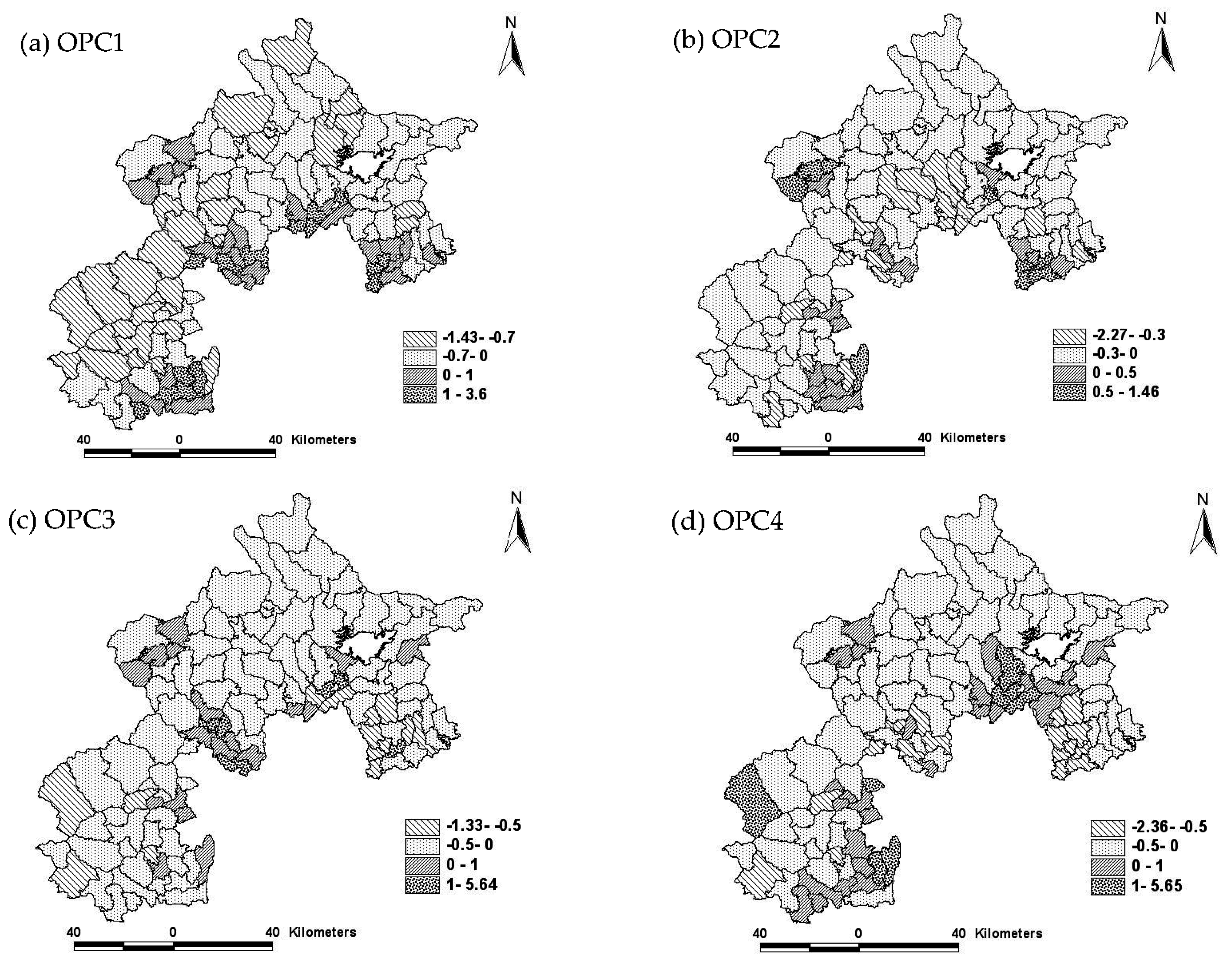
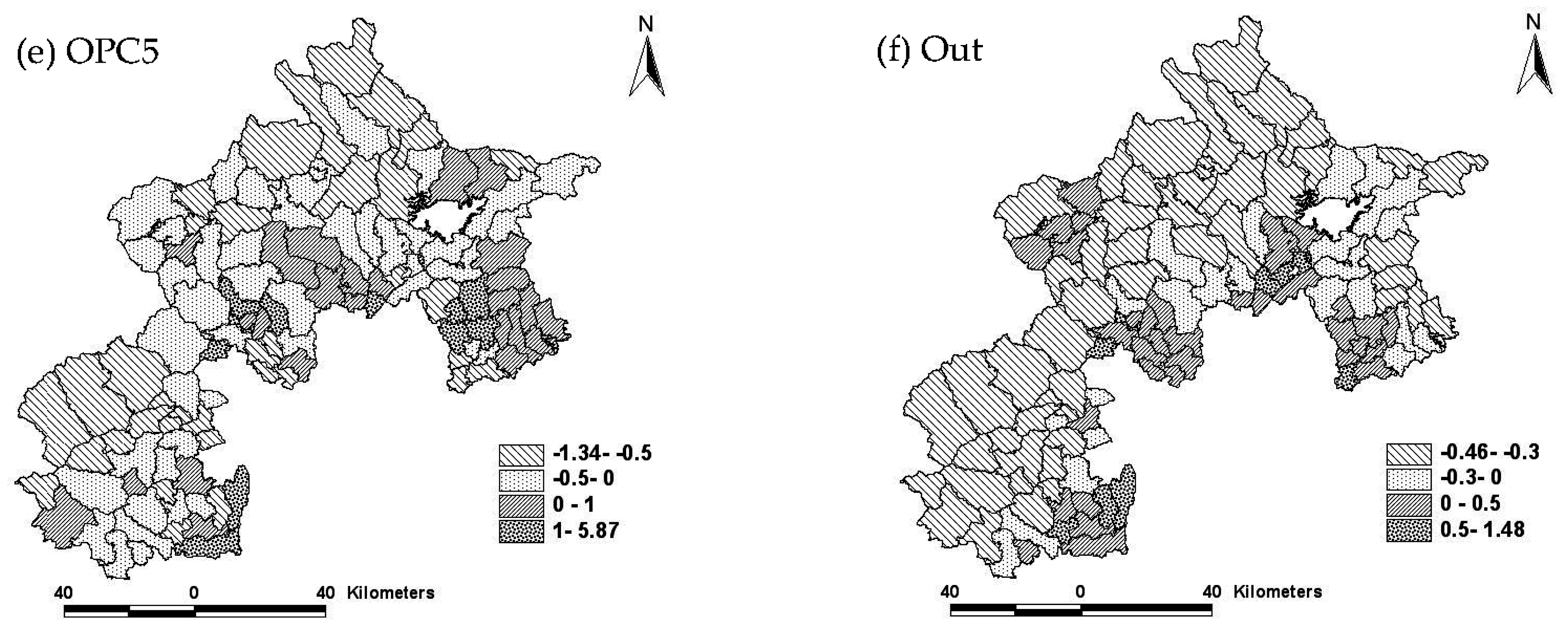
Land use intensity can be defined in a number of ways. In this study, we define it to be a combination of major agricultural inputs and outputs that are directly measured in emergy analysis, i.e., agriculture input intensity and agriculture output intensity. We used the solar emergy data of agricultural input and output, respectively, as inputs for a principal components analysis (PCA), from which we saved the components with eigenvalues exceeding 1. PCA reduces variables to a smaller number of factors that maximize the variation in common to all variables but that are completely uncorrelated with one another (i.e., are orthogonal in n-space). While PCA creates severe difficulties when used to describe the relationship between independent and dependent variables, it remains very effective for reducing the dimensionality of independent datasets. The reasons for using this statistical method were to reduce the number of input and output variables into an “index” of input intensity and output intensity. The Anderson-Rubin method [28], which ensures the orthogonality of the factors, was used to calculate the component scores in PCA. The scores have a mean of 0, a standard deviation of 1, and are uncorrelated. To further combine different input and output intensities, the selected components were integrated as one index (In or Out) using the following equation with their eigenvalues as weights:

$$T\mathrm{int}={\displaystyle \sum _{i=1}^n{\lambda }_i\times p{c}_i}/{\displaystyle \sum _{i=1}^n{\lambda }_i}$$

(1)

where $T\mathrm{int}$ is the integrated index In or Out, and ${\lambda }_i$ is the eigenvalue of an extracted principal component $p{c}_i$.

Before PCA, the Kolmogorov-Smirnov (K-S) statistics were used to test the goodness-of-fit of the data to a log-normal distribution. According to the K-S test, all of the variables are log-normally distributed with 95% or higher confidence. To examine the suitability of the data for PCA, Kaiser-Meyer-Olkin (KMO) and Bartlett’s test were performed. KMO is a measure of sampling adequacy that indicates the proportion of variance which is common variance, i.e., which might be caused by underlying factors. A high value (close to 1) generally indicates that PCA may be useful, which is the case in this study: KMO = 0.76. Bartlett’s test of sphericity indicates whether correlation matrix is an identity matrix, which would indicate that variables are unrelated. The significance level which is 0 in this study (less than 0.05) indicates that there are significant relationships among variables.

2.4. Land Capability Overall Index (LCI) and Emergy Sustainability Index (ESI)

A land capability classification map of the study areas was created using a land use map derived from image processing and interpretation of Landsat-8, based on the effects of combinations of climate and permanent soil characteristics on the productive capacity, limitations of use, and risks of land degradation, particularly water erosion and fertilization degradation (Figure 2). The land capability classification map contained grid data with 30m resolution. The relative coverage area for each land capability class in the study areas is presented in

Table 2. Area percentage of study area for each land capacity class and its Land Capability Overall Index (LCI) weight.

Land Capacity	Class I	Class II	Class III	Class IV	Class V	Class VI	Class VII	Class VIII	Others
Area percent (%)	5.84	10.63	17.68	19.63	21.72	9.42	2.14	0.17	12.77
Weight	0.98	0.90	0.75	0.60	0.50	0.40	0.20	0.10	0

. The highest land quality (class I–class II) was found on the plains close to urban areas and accounted for only 16.47% of the whole study area, a moderate land quality (class III–class V) was mainly found in the foothills and basin of the Beijing mountainous region and accounted for 59.03% of the study area, and the poorest land quality was found for the moderate mountain terrain and accounted for 11.56% of the study area.

In this study, the data analyses were performed at the town level. Thus, the LCI for each town, which reflects the regional land resources quality, were calculated through the following equation:

$$LCI={\displaystyle \sum \%L{C}_i}\cdot W_i$$

(2)

where $\%L{C}_i$ is the percentage of the total area occupied by the land capability class $i$ at the town level and $W_i$ is the weight for land capability class $i$, which is obtained using its potential productivity and local expert knowledge (Table 2). As such, the LCI is an area-weighted average to reflect the overall status of land quality, and the higher the LCI, the higher the land potential.

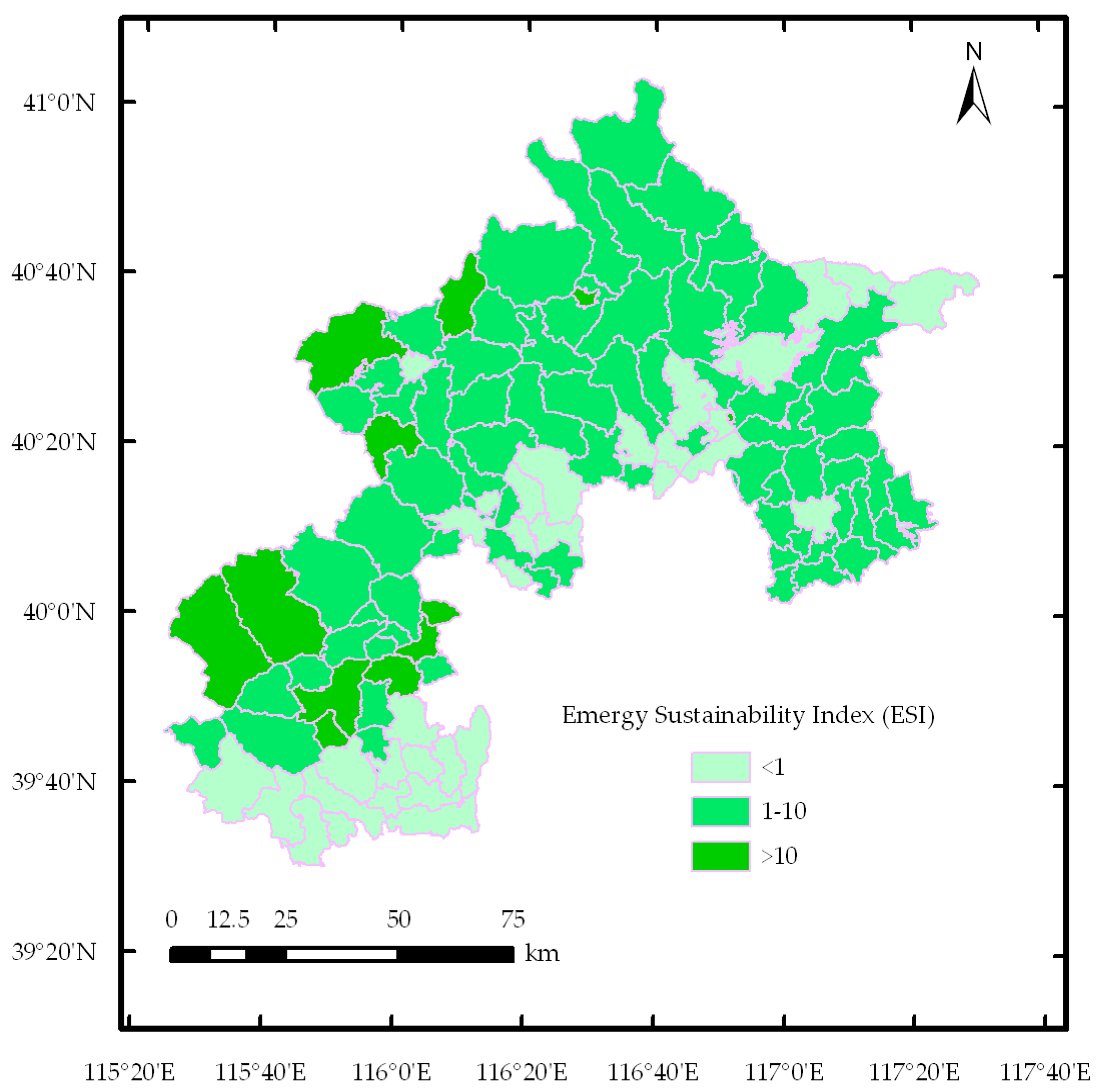
The emergy sustainability index (ESI), that is one of basic emergy indices, was calculated as [19]:

ESI = EYR/ELR
EYR = Y/(NP + RP)
ELR = (NP + NR)/(RR + RP)

(3)

where EYR is the emergy yield ratio, and ELR is the environmental load ratio which expresses the use of environment services by a system, indicating a load on the environment. Y, NP, RP, NR, RR are explained in Table 1. The larger the ESI, the higher the sustainability of a system.

2.5. Data Analyses

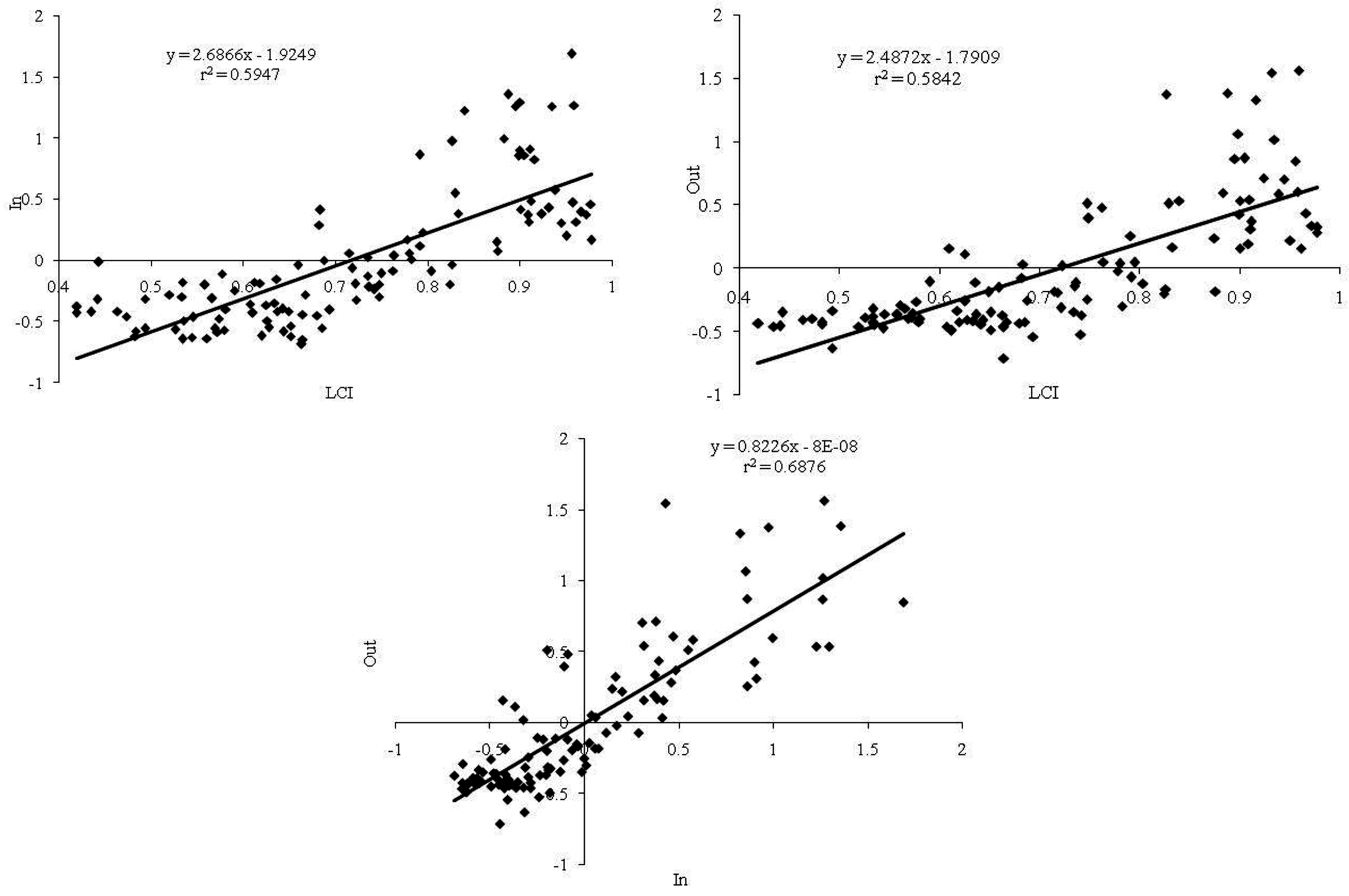
The correlation analysis and regression analysis have been widely used in land use research. In this study, correlation analysis was conducted for the indices LCI, In, Out, and ESI to verify whether they were reasonably dependent on one another. A regression analysis was applied to examine the relationships between the LCI, In, Out, and ESI.

Cluster analysis is a group of multivariate techniques whose primary purpose is to assemble objects based on the characteristics they possess. Cluster analysis classifies objects, so that each object is similar to the others in the cluster with respect to a predetermined selection criterion. The resulting cluster of objects should then exhibit high internal (within-cluster) homogeneity and high external (between clusters) heterogeneity. K-means clustering is the most common and fastest approach, which aims to partition n observations into k clusters in which each observation belongs to the cluster with the nearest mean. When the number of clusters is fixed to k, k-means clustering gives a formal definition as an optimization problem: finding the k cluster centers and assigning the objects to the nearest cluster center, such that the squared distances from the cluster are minimized. In this study, the LCI, In, Out, and ESI were used as independent variables in a cluster analysis (k-means algorithm) in order to aggregate towns into zones of similar agricultural land use intensity. The k value minimizing the sum of squares due to error (SSE) was identified as the number of agricultural land use intensity types through trying different k values. The purpose of using the k-means algorithm was to collapse the number of towns into fewer groups, which could then be analyzed in more detail.

The above statistical analyses were performed with the SPSS 13.0 software (International Business Machines Corporation, Armonk, NY, USA).

3. Results and Discussion

3.1. Input and Output Intensity Indices

Five components were extracted from the input factors and five components were extracted from the output factors for 112 towns. Their eigenvalues and eigenvectors are given in

Table 3. Eigenvalues of the extracted input and output components.

	Components	Eigenvalue	Proportion %	Cumulative %
Input intensity	1	4.92	35.16	35.16
	2	1.83	13.07	48.24
	3	1.58	11.31	59.55
	4	1.48	10.59	70.14
	5	1.43	10.22	80.36
Output intensity	1	2.62	21.84	21.84
	2	2.02	16.86	38.70
	3	1.37	11.41	50.11
	4	1.29	10.74	60.85
	5	1.14	9.53	70.37

,

Table 4. Weights reflect which are the main important variables of each input principal components in the study area.

Components	1	2	3	4	5
Sunlight	−0.19	−0.82	0.10	−0.15	−0.01
Rain, chemical energy	0.19	0.86	0.12	0.05	0.03
Soil loss	0.09	0.55	0.30	−0.52	−0.17
Nitrogen fertilizer	0.94	0.10	0.09	0.06	0.10
Phosphorus fertilizer	0.93	0.03	−0.05	−0.08	−0.01
Potash fertilizer	0.92	−0.01	0.00	−0.06	0.00
Compound fertilizer	0.91	0.11	0.11	0.07	0.07
Pesticides	0.37	0.14	0.58	−0.05	−0.03
Agricultural plastic mulch	0.13	−0.06	0.82	0.07	0.14
Mechanized power	0.19	0.16	0.13	0.87	0.04
Electricity use	0.13	0.00	0.09	0.81	0.11
Human labor	0.49	0.19	0.59	0.50	0.17
Organic manure	0.50	−0.03	0.20	0.36	0.65
Seed	0.86	0.12	0.18	0.15	0.04

and

Table 5. Weights reflect which are the main important variables of each output principal components in the study area.

Components	1	2	3	4	5
Grain crops	0.83	0.16	0.11	0.09	0.03
Oil crops	0.16	−0.06	−0.03	0.82	−0.02
Vegetables	0.29	0.89	0.13	−0.09	−0.06
Fruits	0.01	−0.11	−0.08	−0.14	0.81
Pork	0.68	0.44	0.24	0.13	0.08
Beef	0.74	0.01	0.06	0.27	−0.15
Mutton	0.50	−0.23	0.05	−0.05	0.32
Fowl	0.19	0.04	0.90	−0.12	0.06
Milks	0.36	0.09	0.63	0.44	−0.06
Eggs	0.07	0.94	−0.05	0.00	0.02
Forest logging	0.00	0.21	0.20	0.35	0.57
Fish	0.43	0.14	−0.06	−0.40	−0.09

. The five extracted input components explained 80.36% of the variation in the input intensity (Table 3) and they were combined to express the input intensity index (In) (Figure 3). The five extracted output components explained 70.37% of the variation in output intensity (Table 3), and they were likewise combined as one output intensity index (Out) (Figure 4).

The first principal component of the input intensity (IPC1) accounted for 35.16% of the total variation in the data (Table 3), with chemical fertilizer and seed being the largest inputs in the Beijing mountainous agricultural system (Table 4). The higher IPC1 mainly focused on the flood and alluvial plain of Beijing (Figure 3a), where the central regions for a large amount crop production, radiation zone of urban construction and human inhabitation are located. The second principal component of the input intensity (IPC2), which accounted for 13.07% of the total variation, had high positive weights for rain chemical energy, soil loss, and high negative weights for sunlight. Thus, the IPC2 expressed the effects of natural resources on agricultural production, with soil loss due to erosion and a shortage of sunlight considered the major natural limitations in the Beijing mountainous agricultural system. The third principal component of the input intensity (IPC3) had high positive weights for agricultural plastic mulch, human labor, and pesticides, which showed tied ridges, with plastic mulch technology widely adopted to maintain soil temperature and moisture along with high pesticide use and labor input for agricultural production. The fourth principal component of the input intensity (IPC4) had high positive weights for mechanized power, electricity use, human labor, and a high negative weight for soil loss, indicating that there is a lower risk of soil loss, higher level of mechanization, and more industrialized agricultural production. The fifth principal component of the input intensity (IPC5) had a high positive weight for organic manure, indicating that organic manure as an environmentally friendly source of nutrients was still a source of nutrient input. However, artificial chemical fertilizer was widely used as the principal agricultural input in the study areas. The structure of input intensity indicates that non-renewable energy was the overwhelming input for the agriculture systems.

Table 5 shows the first principal component of the output intensity (OPC1), which accounts for 21.84% of the total variation in the output data, had high positive coefficients for grain crops, beef, pork, and fish, and reflected that grain and meat were the main product outputs in the study areas, which were mainly produced from urban fringe of Beijing, i.e., mountainous areas near the Beijing plain (Figure 4a). Eggs and vegetables were the secondary product outputs and associated with the second principal component of output (OPC2), which accounted for 16.86% of the total variation. The third principal component of output intensity (OPC3) was fowl, milk, and oil crops (OPC4), and fruits (OPC5) were the important product outputs of the agricultural system. With the enforcement of ecological protection, forest logging decreased in the study areas (Table 5).

Table 6. Bivariate correlation coefficients of input and output principal components.

	IPC1	IPC2	IPC3	IPC4	IPC5	OPC1	OPC2	OPC3	OPC4	OPC5
IPC1	1	0.00	0.00	0.00	0.00	0.65 a	−0.01	0.22 b	0.38 a	0.10
IPC2	0.00	1	0.00	0.00	0.00	0.23 b	0.18 b	−0.01	0.22 b	0.20 b
IPC3	0.00	0.00	1	0.00	0.00	0.23 b	0.57 a	0.11	−0.02	0.24 b
IPC4	0.00	0.00	0.00	1	0.00	0.19 b	0.06	0.07	0.01	−0.02
IPC5	0.00	0.00	0.00	0.00	1	0.22 b	−0.03	0.65 a	−0.16	−0.01
OPC1	0.65 a	0.23 b	0.23 b	0.19 b	0.22 b	1	0.00	0.00	0.00	0.00
OPC2	−0.01	0.18 b	0.57 a	0.06	−0.03	0.00	1	0.00	0.00	0.00
OPC3	0.22 b	−0.01	0.11	0.07	0.65 a	0.00	0.00	1	0.00	0.00
OPC4	0.38 a	0.22 b	−0.02	0.01	−0.16	0.00	0.00	0.00	1	0.00
OPC5	0.10	0.20 b	0.24 b	−0.02	−0.01	0.00	0.00	0.00	0.00	1

^a Significant at the 0.01 significance level (two-tailed); ^b Significant at the 0.05 significance level (two-tailed), and the number of towns (n) is 112.

shows the correlation coefficients of the principal components of input and output. OPC1 had a significant positive correlation with IPC1 at the 0.01 significance level and significant positive correlations with the other input indices at the 0.05 significance level. These correlations indicate that grain production in the study areas was mainly dependent on the artificial fertilizer input and the major limitations for grain production were soil loss and a shortage of sunlight. Since meat husbandry relied on grain crops, it was significantly correlated with the input indices. OPC2 had a significant positive correlation with IPC3 and a positive correlation with IPC2, which indicated that vegetable production and egg husbandry required high inputs of labor and pesticides and ridges and/or greenhouses with plastic mulch were widely adopted in vegetable production to compensate for natural resource limitations, particularly sunlight. OPC3 had high significant positive correlations with IPC5 and IPC1, indicating that fowl husbandry and milk husbandry depended on grain crop production and their by-products were returned to grain crop production as organic manure. Oil crop production also depended on artificial fertilizer input and was limited by sunlight with the risk of soil loss, which was reflected in its significant correlations with IPC1 and IPC2. OPC5 had significant positive correlations with IPC3 and IPC2, which indicated that fruit production also needed high amounts of labor and pesticides and faced the risk of soil loss and limited sunlight.

Figure 5 shows that the gross value of agricultural output in the study area increased quickly, due to arable land resources in the Beijing plain region converting to non-agricultural land because of city sprawl, particularly in the high-development periods of the previous ten years. However, the increase in agricultural output was dependent on a large amount of non-renewable resources to yield staple crops, meat, and vegetables according to the above analyses of agricultural inputs and outputs.

3.2. ESI

Figure 6 shows the ESI of each town in the study areas. An ESI of less than one indicates a fragile agro-ecological environment, and such environments are mainly on the plains surrounding urban areas and the northeast upstream of the Miyun Reservoir. An ESI of between one and ten indicates that agricultural system has vitality and potential, and An ESI of larger than ten indicates a higher sustainability of agricultural system.

3.3. Relationships of the LCI, In, Out, and ESI

There was a highly significant positive correlation among the In, Out, and LCI indices, whereas the ESI index had a significant negative correlation with each of them (

Table 7. Bivariate correlation coefficients of indices.

	LCI	In	Out	ESI
LCI	1	0.75 a	0.76 a	−0.21 b
In	0.75 a	1	0.84 a	−0.45 a
Out	0.76 a	0.84 a	1	−0.30 a
ESI	−0.21 b	−0.45 a	−0.30 a	1

^a Significant at the 0.01 significance level (two-tailed); ^b Significant at the 0.05 significance level (two-tailed).

), thus there was a better natural land quality, a higher agricultural input intensity, and a greater agricultural output. However, the sustainability of the agricultural system was low. The better land, which needs fewer purchased resources, such as fertilizer and labor, than low quality land, can reduce the farmers input cost and make higher marginal returns. Therefore, most farmers prefer to put the higher inputs on the best land, rather than use them to remediate the poor land in the study area.

To further examine the relationships of the indices, regression analyses were performed for the three pairs: In versus LCI, Out versus LCI, and Out versus In. The regression lines were separately obtained (Figure 7). There was a good fitting linear relationship between the In and LCI (r² = 0.59, p < 0.001), Out and LCI (r² = 0.58, p < 0.001), and Out and In (r² = 0.68, p < 0.001). Figure 7 shows that in the study areas, the agricultural output intensity varied even for the same land quality and input intensity. Furthermore, the same land quality had diverse input intensity.

Multiple regression models of the ESI obtained from multiple regression analyses between the ESI and LCI, In and Out are listed in

Table 8. Multiple regression models of the ESI.

	Variable in Equation	Adjusted R2	Standardized Beta	Number of Samples
1 (normal)	In	0.403	−0.893	82
	Out		0.339
2 (outliers) *	In	0.296	−1.728	30
	Out		1.603

* Outliers: outside the range of ±2 standard deviations.

. The two variables In and Out were entered in the regression model, while variable LCI were not entered in the regression model. This shows that agricultural input intensity and agricultural output intensity had greater effects on the sustainability of the agricultural system. Higher agricultural output and lower agricultural input could bring higher efficiency of the agricultural system. Therefore, a high rate of transformation from agricultural input to output will promote the sustainability of an agricultural system. However, in the study areas, most of the towns (82) had a low transformation rate (Table 8).

3.4. AgriculturalIntensity Types and Their Assessment

Whether agricultural land use intensity would be suitable to land capability is vital for regulating agricultural resources. For the same land quality and input intensity, higher output intensity and ESI are desired. To explore the spatial distribution of the relationship among agricultural land use intensity, land capability and agricultural sustainability, the k-means cluster analysis delineated eight types of agricultural intensity, which had robust similarities in the LCI, In, Out, and ESI (Figure 8 and

Table 9. Agricultural intensity indices and economic factors for the eight types of intensities.

	Type 1	Type 2	Type 3	Type 4	Type 5	Type 6	Type 7	Type 8
LCI	0.63	0.62	0.54	0.71	0.70	0.91	0.89	0.90
In	−0.17	−0.37	−0.47	−0.19	0.20	0.35	0.30	1.02
Out	−0.31	−0.32	−0.35	0.19	−0.10	0.19	0.41	0.84
ESI	0.45	4.19	16.92	3.29	0.82	0.68	2.02	0.60
Gross value of agricultural output (million CNY *)	30.97	29.26	18.76	73.50	46.73	67.28	77.28	85.60
GDP per capita (CNY *)	7464	7964	7653	10,014	8378	13,502	11,178	12,198
Number of towns	6	46	9	7	7	8	14	15

* CNY: Chinese Yuan Renminbi.

).

Types 1, 2, and 3 were the lowest agricultural land use intensities and land capabilities of the study areas. The three types were mainly located in the mountainous areas and the low land capability limited the land use intensity. However, areas of type 1 intensity had smaller ESI values, indicating that they relied more on purchased energy and non-renewable resource inputs. Therefore, the structure of agriculture and input intensity should be adjusted in such areas to increase the ESI, particularly in towns in the northeast upstream of the Miyun Reservoir, which supplies domestic water to Beijing City (Figure 8). It should adjust artificial chemical material input intensity to avoid the surpluses. Since 2003, the government of Beijing has reduced livestock and fisheries in the Beijing mountainous region, but the artificial chemical material input did not draw attention. Moreover, the development of more ecologically-designed agricultural systems that reintegrate features of traditional agricultural knowledge and add new ecological knowledge into the intensification process based on the mountainous land resources can contribute to meeting this challenge. Areas with type 2 intensity were relatively well managed with a balance in the LCI, land use intensity, and ESI. Type 3 intensity was seen in the highest mountainous areas with the lowest land quality, so high agricultural land intensity was not suitable in these areas. The agricultural structure has been changed so that an ecological output has been achieved in recent years, which means that the areas having the lowest gross value of agricultural output had a relatively high GDP per capita (Table 9), so the low land intensity with a high ESI should be maintained.

Type 4 intensity was seen in the Yanqing Basin and represented a low input and moderate output intensity with an LCI of 0.71. Thus, there was a high change rate pattern and the ESI was between 1 and 10, which indicated a high level of sustainability. Therefore, this pattern should be maintained for the Yanqing Basin, which has a good environmental condition, is surrounded by mountains, and has a good economy with a high gross value of agricultural output and GDP per capita. Currently, the basin provides increasing amounts of vegetables and grain, with Beijing City sprawl resulting in a resource loss in the plains. Areas of type 5 intensity had land resources similar to the resources of areas of type 4, but they had low output with moderate input intensity. The total output value of agriculture for areas of type 5 intensity was low. For the land with moderate LCI (0.70), bad management and extensive land use maybe cause low agricultural outputs. Moreover, the low level of input resources utilization is another reason for the moderate input and low output. The excessive inputs to agricultural ecosystem could certainly result in energy accumulation and surplus; consequently leading to an increasing load on the environment. Thus, poor management of land use intensity also increased the load on the environment, which produced an ESI value of 0.82, and areas of type 5 intensity should follow the type 4 pattern for sustainability.

Areas with type 6, 7, and 8 intensities had the best land quality in the study areas and were located on the plains close to urban areas. Among them, areas of type 8 intensity had the highest agricultural input and output intensities of the study areas. Although this high agricultural land use intensity was relatively reasonable in terms of the high land capability, the ESI was less than one with heavy stress to the regional environment. Thus, there should be a greater input of renewable energy (such as organic manure) in place of non-renewable energy (such as chemical fertilizer). Areas with type 6 and 7 intensities had moderate agricultural input and output intensities that did not match the land quality. There was less output and a smaller ESI for areas with type 6 intensity than areas with type 7 intensity. The type 6 and 7 intensity areas were in the main expansion region of the city. Since reform and opening to the outside world in 1978, Beijing has experienced high-speed urbanization and economic growth, and the rapid urbanization process in these thirty years has brought an unparalleled scale and rate of urban sprawl, which has caused that large amount of agricultural land in the Beijing alluvial plain lost. As a result, farmers in the main expansion region reduced inputs to their land and were less concerned with agricultural outputs. The gross agricultural output for areas with type 6 intensity was relatively low, whereas the GDP per capita was relatively high.

4. Conclusions

Land use intensity has become a hot topic in land use and land cover change research, and it often, although not exclusively, refers to agriculture. Using the Beijing mountainous region as a case study, the spatial distributions of agricultural land use intensity were determined using an emergy analysis through PCA and k-means clustering methods. The extracted principal components could help determine the agricultural input and output structure of Beijing mountainous region. The study indicated that the emergy methodology could integrate analytical data into a common unit basis, making the results more usable. Therefore, characterizing agricultural land use intensity based on an ecological assessment method provides an overall assessment of regional land use intensity.

Correlation and regression analyses were used to determine the relationship between land capability, agricultural input intensity, and agricultural output intensity. The correlation patterns and regression modeling obtained from this study can help to understand land use intensity. In the future, research efforts will be on going to discover the further relationship among agricultural input intensity, agricultural output intensity, land capability, and agricultural system sustainability. In the assessment of the eight agricultural land use intensities, the agricultural land use intensity should be suitable to the land capability, and the agricultural output intensity should be high with low agricultural input intensity to maintain the sustainability of an agricultural system.

The results of this study demonstrate the usefulness of a tool for characterizing and assessing agricultural land use intensity in the Beijing mountainous region. It can be used to help urban planners, managers, and decision-makers monitor, adjust, and control the sustainable development of agricultural land use in the Beijing mountainous region.

References

1. Galicia, L.; Romero, A.G. Land use and land over change in highland temperate forests in the Izta-Popo national park, central Mexico. Mt. Res. Dev. 2007, 27, 48–57. [Google Scholar] [CrossRef]
2. Lambin, E.F.; Rounsevell, M.D.A.; Geist, H.J. Are agricultural land-use models able to predict changes in land-use intensity? Agric. Ecosyst. Environ. 2000, 127, 321–331. [Google Scholar] [CrossRef]
3. Turner, B.L.; Doolittle, W.E. The concept and measure of agricultural intensity. Prof. Geogr. 1978, 30, 297–301. [Google Scholar] [CrossRef]
4. Brookfield, H.C. Notes on the theory of land management. PLEC News Views 1993, 1, 28–32. [Google Scholar]
5. Kates, R.W.; Hyden, G.; Turner, B.L. Population Growth and Agricultural Change in Africa; University Press of Florida: Gainesville, FL, USA, 1993. [Google Scholar]
6. Netting, R.M. Smallholders, Householders: Farm Families and the Ecology of Intensive, Sustainable Agriculture; Stanford University Press: Palo Alto, CA, USA, 1993. [Google Scholar]
7. Shriar, A.J. Agricultural intensity and its measurement in frontier regions. Agrofor. Syst. 2000, 49, 301–318. [Google Scholar] [CrossRef]
8. Kerr, J.T.; Cihlar, J. Land use and cover with intensity of agriculture for Canada from satellite and census data. Glob. Ecol. Biogeogr. 2003, 12, 161–172. [Google Scholar] [CrossRef]
9. Herzog, F.; Steiner, B.; Bailey, D.; Baudey, J.; Billeter, R.; Bukacek, R.; De Blust, G.; De Cock, R.; Dirksen, J.; Dormann, C.F.; et al. Assessing the intensity of temperate European agriculture at the landscape scale. Eur. J. Agron. 2006, 24, 165–181. [Google Scholar] [CrossRef]
10. Tilman, D. Global environmental impacts of agricultural expansion: the need for sustainable and efficient practices. Proc. Natl. Acad. Sci. USA 1999, 96, 5995–6000. [Google Scholar] [CrossRef] [PubMed]
11. Krausmann, F.; Haberl, H.; Erb, K.-H.; Wackernagel, M. Resource flows and land use in Austria 1950–2000: Using the MEFA framework to monitor society-nature interaction for sustainability. Land Use Policy 2004, 21, 215–230. [Google Scholar] [CrossRef]
12. Wrbka, T.; Erb, K.-H.; Schulz, N.B.; Peterseil, J.; Hahn, C.O.; Haberl, H. Linking pattern and process in cultural landscapes. An empirical study based on spatially explicit indicators. Land Use Policy 2004, 21, 289–306. [Google Scholar] [CrossRef]
13. Zhuang, D.F.; Liu, J.Y. Study on the model of regional differentiation of land use degree in China. J. Nat. Resour. 1997, 12, 105–111. [Google Scholar]
14. Wang, G.J.; Liao, S.G. Spatial heterogeneity of land use intensity. Chin. J. Appl. Ecol. 2006, 17, 611–614. [Google Scholar]
15. Martin, J.F.; Diemont, S.A.W.; Powell, E.; Stanton, M.; Tacher, S.L. Emergy evaluation of the performance and sustainability of three agricultural systems with different scales and management. Agric. Ecosyst. Environ. 2006, 115, 128–140. [Google Scholar] [CrossRef]
16. Odum, H.T. Environmental Accounting: Emergy and Environmental Decision Making; Wiley: New York, NY, USA, 1996. [Google Scholar]
17. Ulgiati, S.; Brown, M.T.; Bastianoni, S.; Marchettini, N. Emergy based indices and ratios to evaluate the sustainable use of resources. Ecol. Eng. 1995, 5, 519–531. [Google Scholar] [CrossRef]
18. Brown, M.T.; Ulgiati, S. Emergy-based indices and ratios to evaluate sustainability: Monitoring economies and technology toward environmentally sound innovation. Ecol. Eng. 1997, 9, 51–69. [Google Scholar] [CrossRef]
19. Ulgiati, S.; Brown, M.T. Monitoring patterns of sustainability in natural and man-made ecosystems. Ecol. Model. 1998, 108, 23–36. [Google Scholar] [CrossRef]
20. Chen, G.Q.; Jiang, M.M.; Chen, B.; Yang, Z.F.; Lin, C. Emergy analysis of Chinese agriculture. Agric. Ecosyst. Environ. 2006, 115, 161–173. [Google Scholar] [CrossRef]
21. Wu, Q.; Li, H.Q.; Wang, R.S.; Paulussen, J.; He, Y.; Wang, M.; Wang, B.H.; Wang, Z. Monitoring and predicting land use changes in Beijing using remote sensing and GIS. Landsc. Urban Plan. 2006, 78, 322–333. [Google Scholar] [CrossRef]
22. Sun, D.F.; Zhou, L.D.; Li, H. Agricultural Resources Sustainable Use and Digital Beijing Mountainous Areas; Research Report; Beijing Academy of Agriculture and Forestry Sciences: Beijing, China, 2004. [Google Scholar]
23. Beijing Municipal Bureau of Statistics. District and County of Beijing Statistical Yearbook 2014; China Statistics Press: Beijing, China, 2014.
24. Odum, H.T.; Brown, M.T.; Brandt-Williams, S. Folio 1: Introduction and Global Budget. Handbook of Emergy Evaluation; Center for Environmental Policy, University of Florida: Gainesville, FL, USA, 2000. [Google Scholar]
25. Cohen, M.J.; Brown, M.T.; Shepherd, K.D. Estimating the environmental costs of soil erosion at multiple scales in Kenya using emergy synthesis. Agric. Ecosyst. Environ. 2006, 114, 249–269. [Google Scholar] [CrossRef]
26. Lan, S.F.; Qin, P.; Lu, H.F. Emergy Analysis of Ecoeconomic System; Chemical Industry Press: Beijing, China, 2002. [Google Scholar]
27. Brown, M.T.; Bardi, E. Folio 3, Emergy of Ecosystems. Handbook of Emergy Evaluation: A Compendium of Data for Emergy Computation Issued in a Series of Folios; Center for Environmental Policy, Environmental Engineering Sciences University of Florida: Gainesville, FL, USA, 2001. [Google Scholar]
28. Anderson, T. An Introduction to Multivariate Statistical Analysis; John Wiley & Sons: New York, NY, USA, 1984. [Google Scholar]
Figure 1. Location of the Beijing mountainous region.
Sustainability 08 01180 g001
Figure 2. Land use map (a) and land capability classification map (b) of the study areas. For map (b), highest land quality (class I–class II); moderate land quality (class III–class V), and low land quality (class VI–class VIII).
Sustainability 08 01180 g002
Figure 3. Map of the input intensity and its five principal components. (a) The first principal component of the input intensity (IPC1); (b) The second principal component of the input intensity (IPC2); (c) The third principal component of the input intensity (IPC3); (d) The fourth principal component of the input intensity (IPC4); (e) The fifth principal component of the input intensity (IPC5); (f) The input intensity index (In).
Sustainability 08 01180 g003
Figure 4. Map of the output intensity and its five principal components. (a) The first principal component of the output intensity (OPC1); (b) The second principal component of the output intensity (OPC2); (c) The third principal component of the output intensity (OPC3); (d) The fourth principal component of the output intensity (OPC4); (e) The fifth principal component of the output intensity (OPC5); (f) The output intensity index (Out).
Sustainability 08 01180 g004aSustainability 08 01180 g004b
Figure 5. Gross agricultural output for the Beijing mountains region. * CNY: Chinese Yuan Renminbi. Date source: Beijing statistical yearbook [23].
Sustainability 08 01180 g005
Figure 6. Emergy sustainability index (ESI) of the study areas.
Sustainability 08 01180 g006
Figure 7. Relationships between the input intensity index (In) and Land Capability Overall Index (LCI), output intensity index (Out) and Land Capability Overall Index (LCI), and output intensity index (Out) and input intensity index (In).
Sustainability 08 01180 g007
Figure 8. Agricultural land use intensity classification in the study areas.
Sustainability 08 01180 g008