
The Optimal Dispatch of a Power System Containing Virtual Power Plants under Fog and Haze Weather

Abstract
: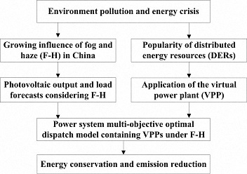
1. Introduction
2. F-H Impacts on Photovoltaic Output and Load Forecasts

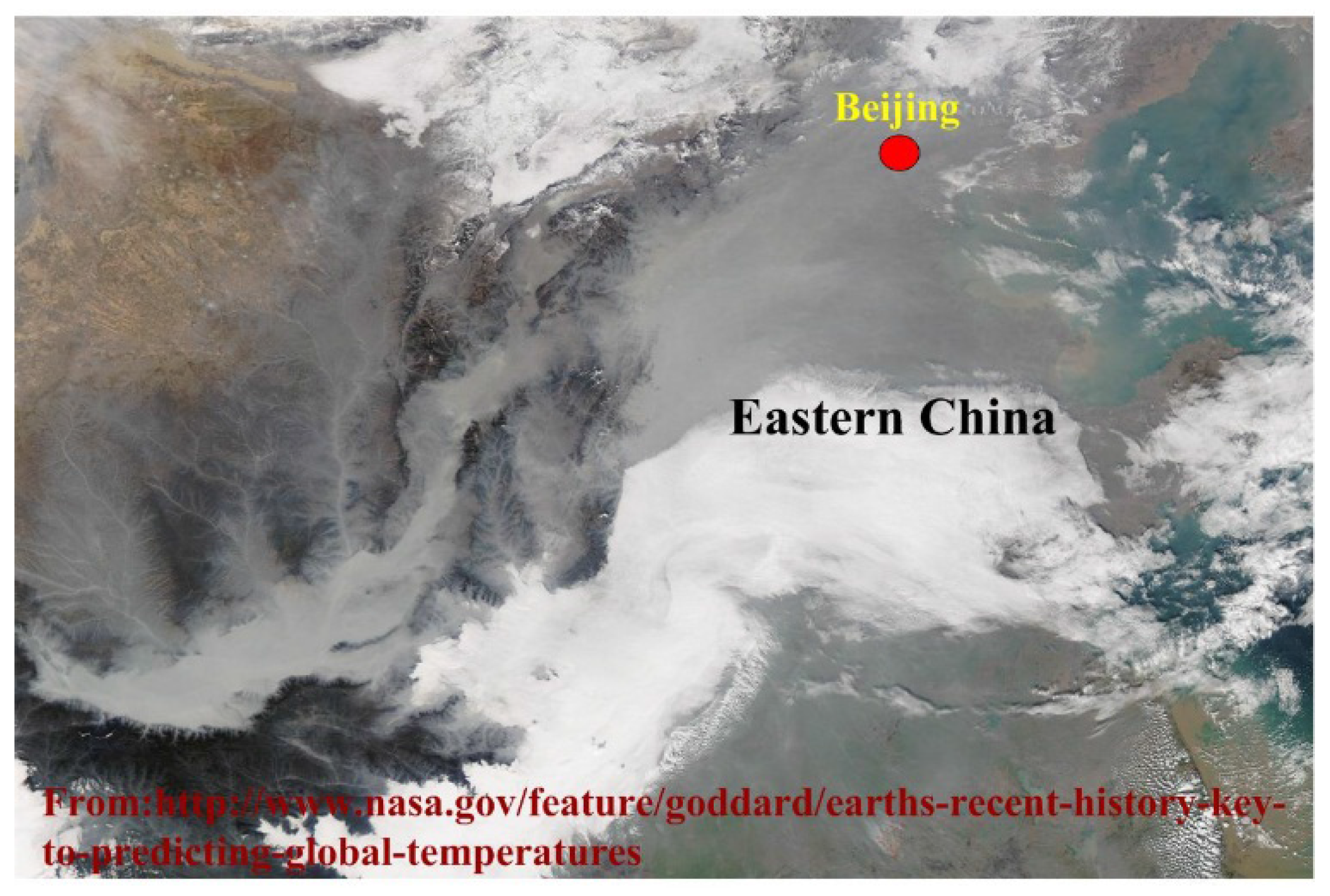
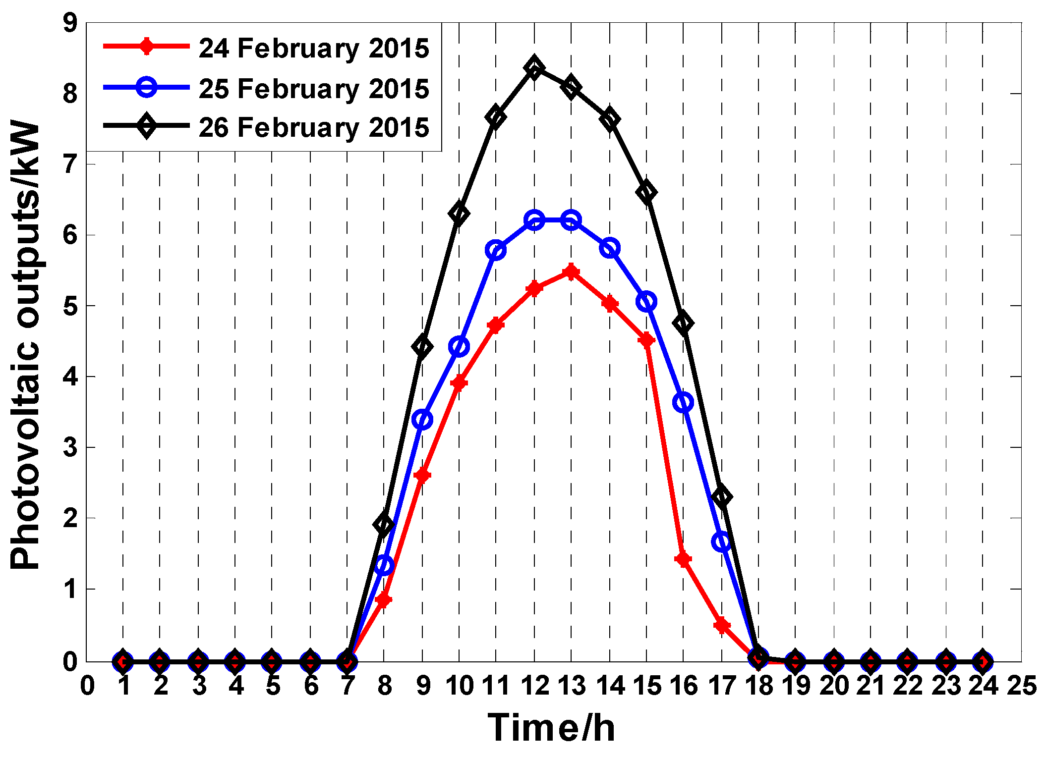
2.1. The Influence of F-H on Photovoltaic Output

| Date | AQI | AQI Level | PM2.5 | PM10 | CO | NO2 | SO2 |
|---|---|---|---|---|---|---|---|
| 24 February 2015 | 337 | Serious/6 | 265 | 442 | 4.13 | 58 | 111 |
| 25 February 2015 | 180 | Moderate/4 | 136 | 247 | 2.2 | 36 | 68 |
| 26 February 2015 | 98 | Good/2 | 68 | 108 | 1.89 | 38 | 92 |

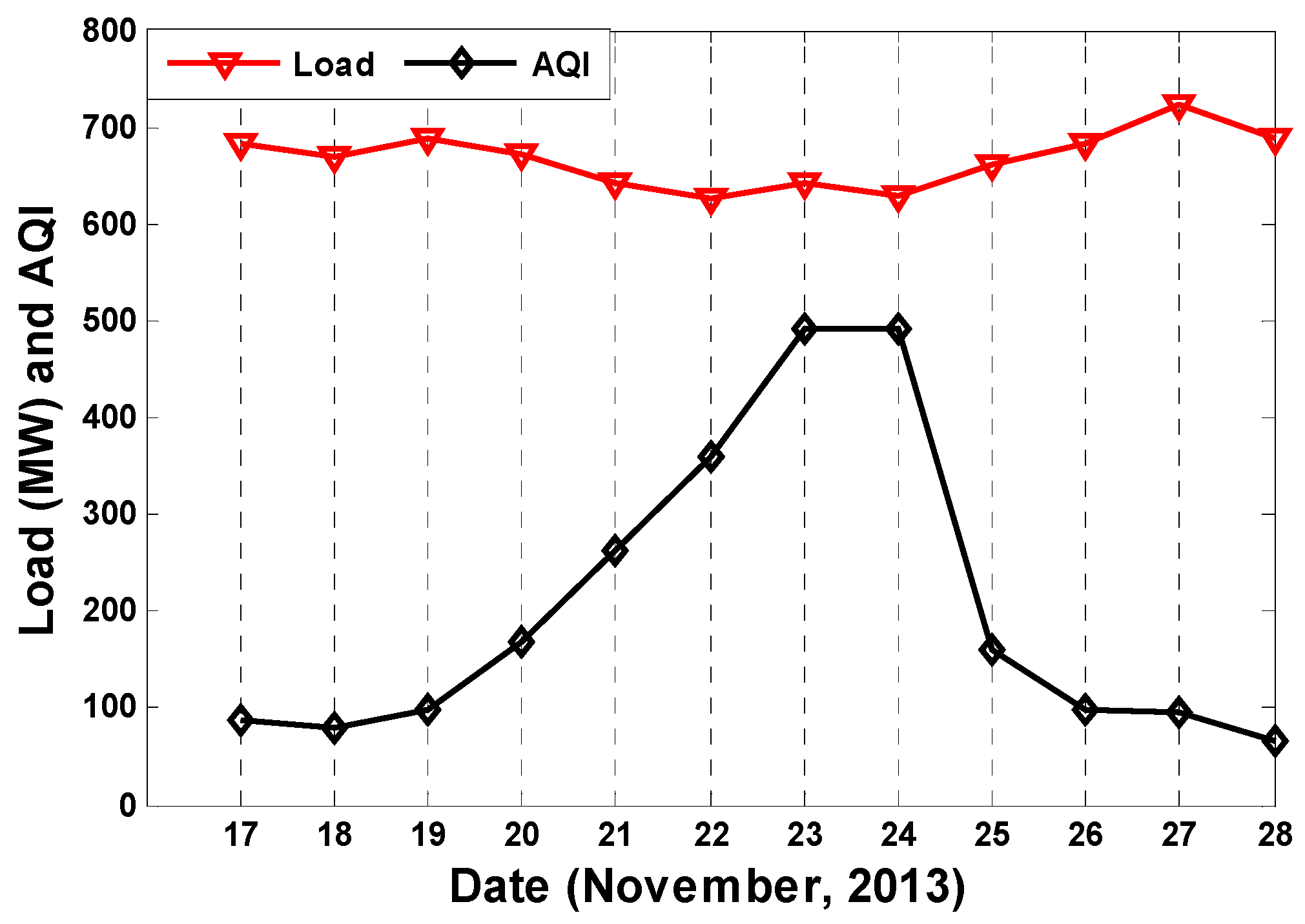
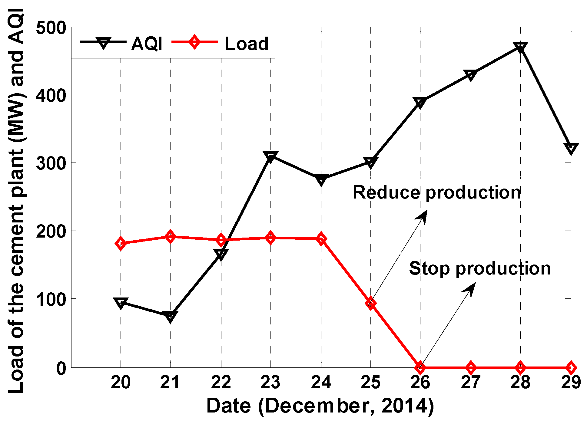
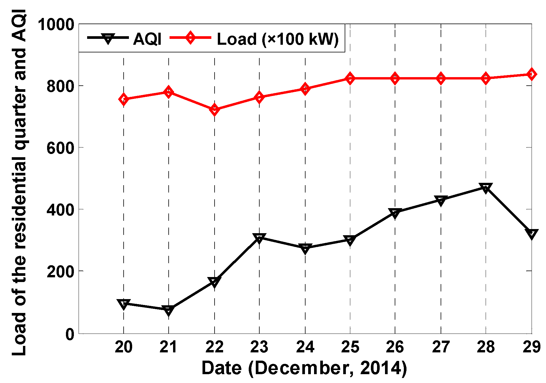
2.2. The Influence of F-H on Load

2.3. Selection of “Similar Days of F-H”
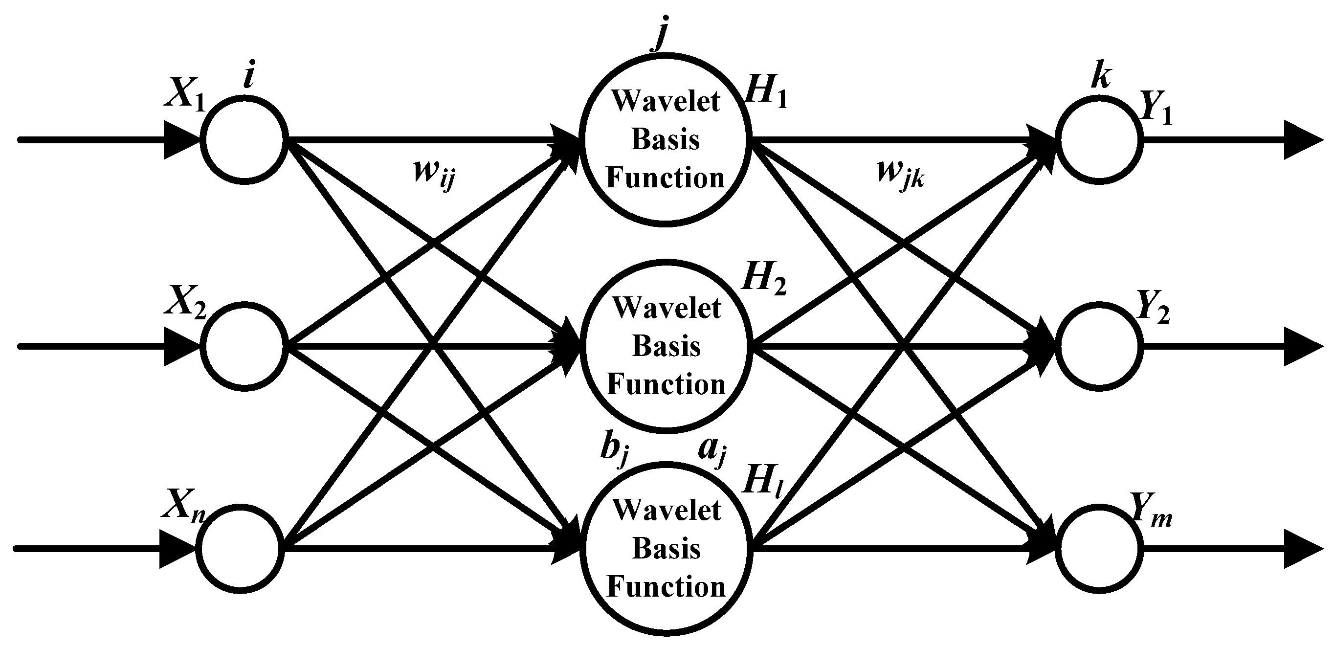
2.4. Prediction Model of the Wavelet Neural Network
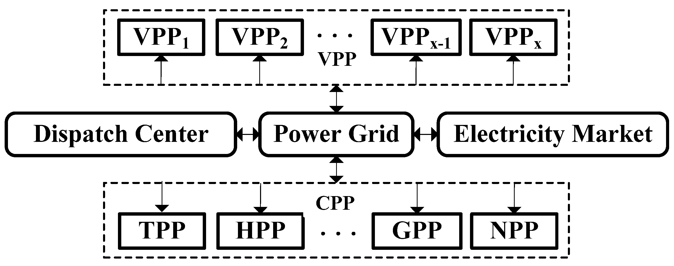
3. The Dispatch of Power Systems Containing VPPs
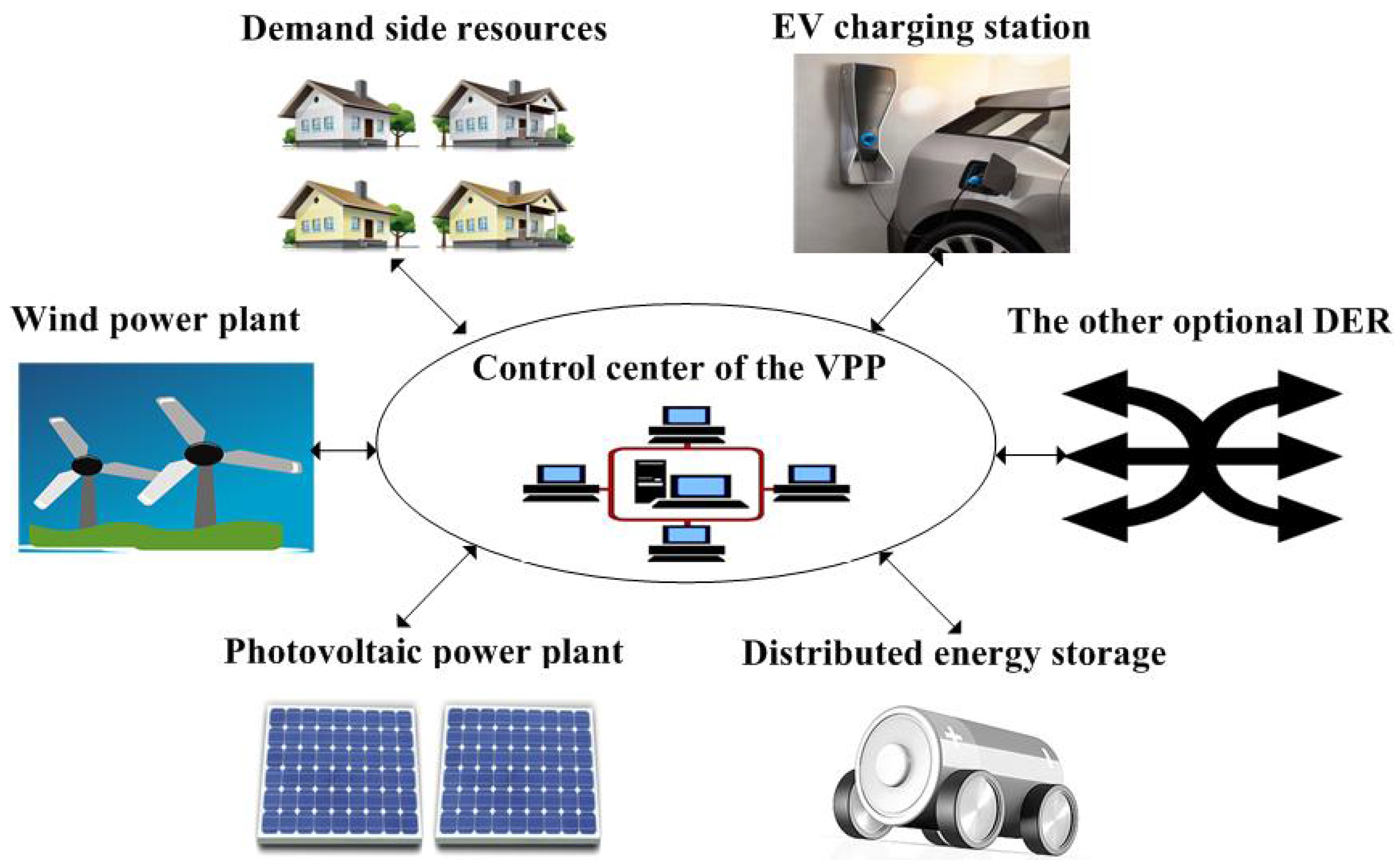
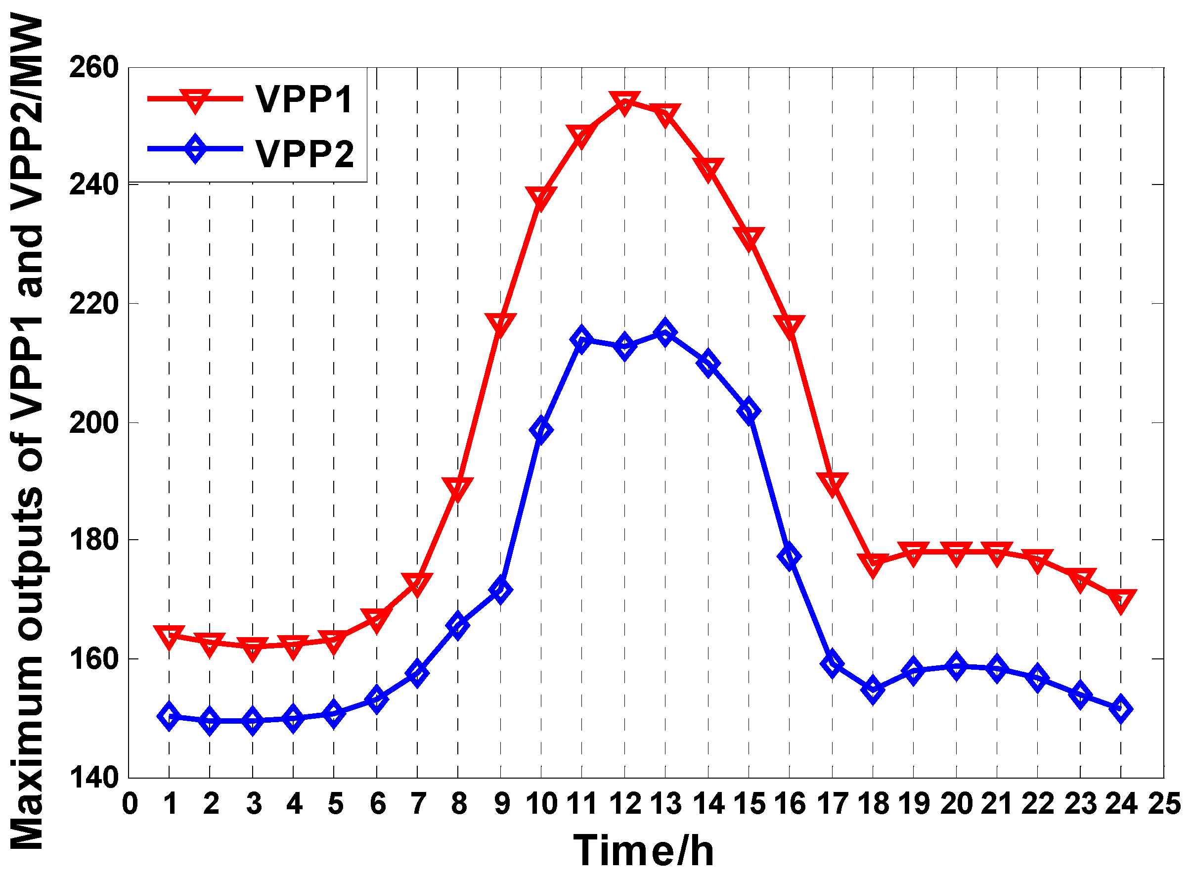
3.1. The Construction of the VPP
3.2. The Dispatch Model Containing VPPs

4. The Mathematical Model of Dispatch under F-H Weather
4.1. Objective Functions
4.2. Constraints
5. Solving the Optimal Dispatch Model Based on MILP
5.1. Model Simplification
5.2. Linearization of Objective Functions
5.3. Model Solving
6. Case Study
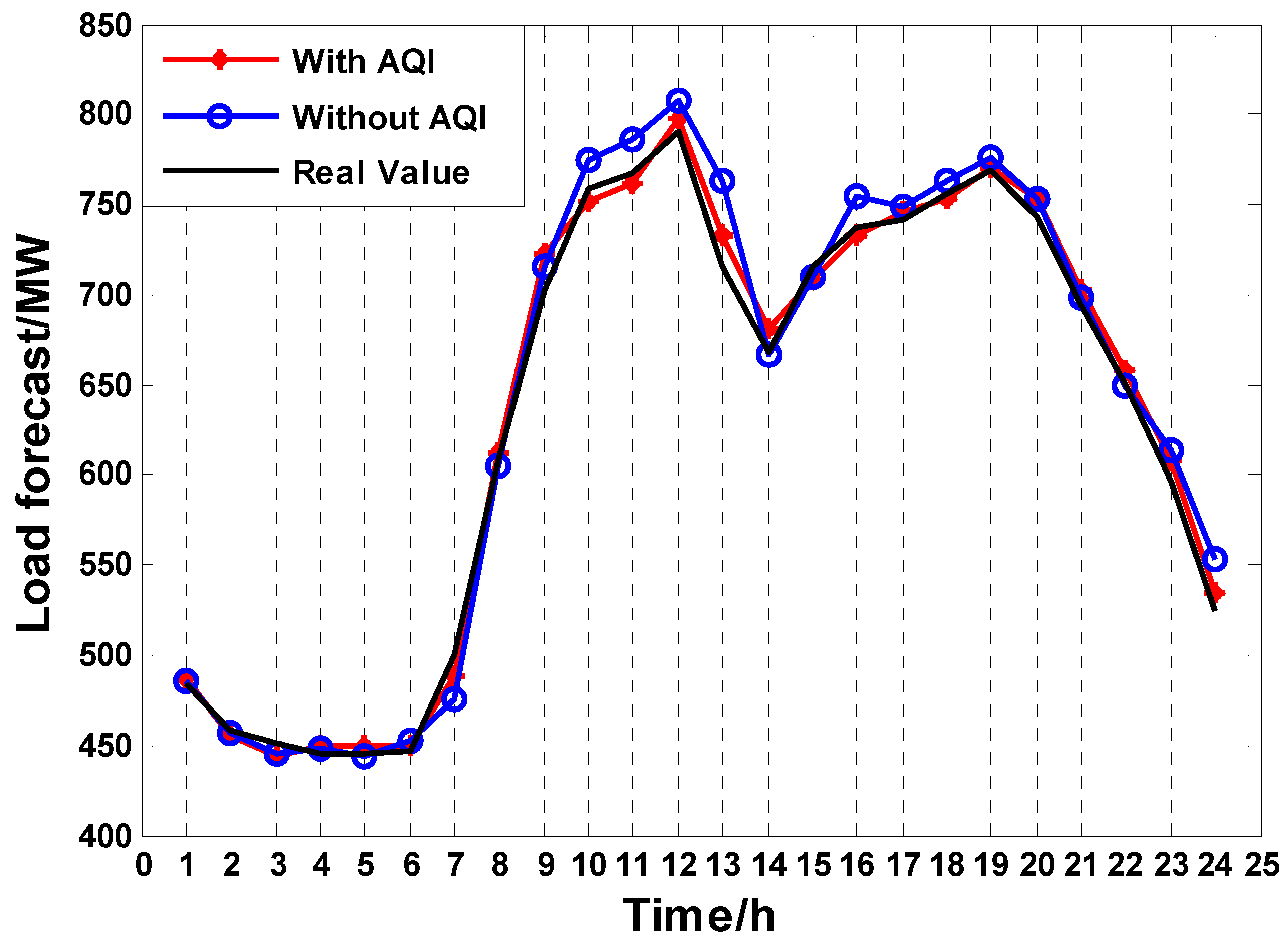
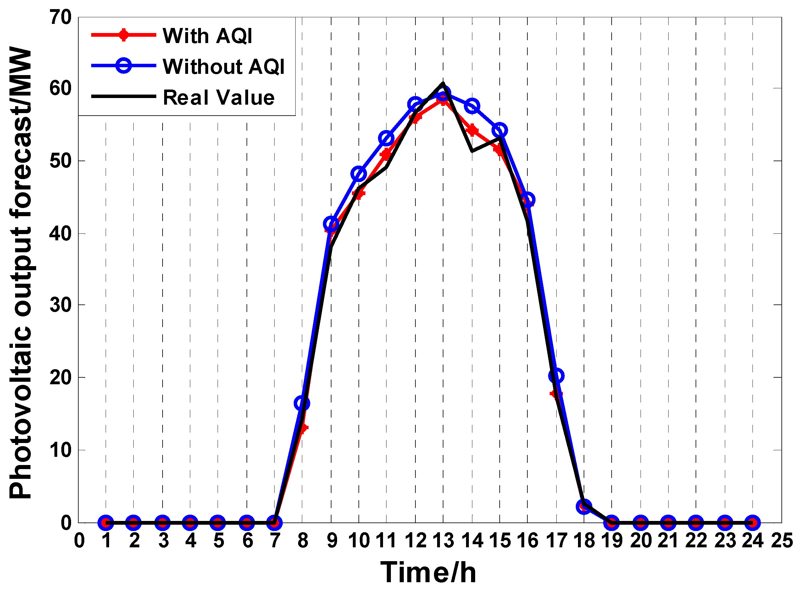
6.1. Photovoltaic Output and Load Forecasts under F-H
| Case | MAPE (%) | MSE |
|---|---|---|
| With AQI | 4.4181 | 2.9696 |
| Without AQI | 8.4941 | 8.5712 |

| Case | MAPE (%) | MSE |
|---|---|---|
| With AQI | 2.6662 | 167.0492 |
| Without AQI | 3.7528 | 523.0842 |
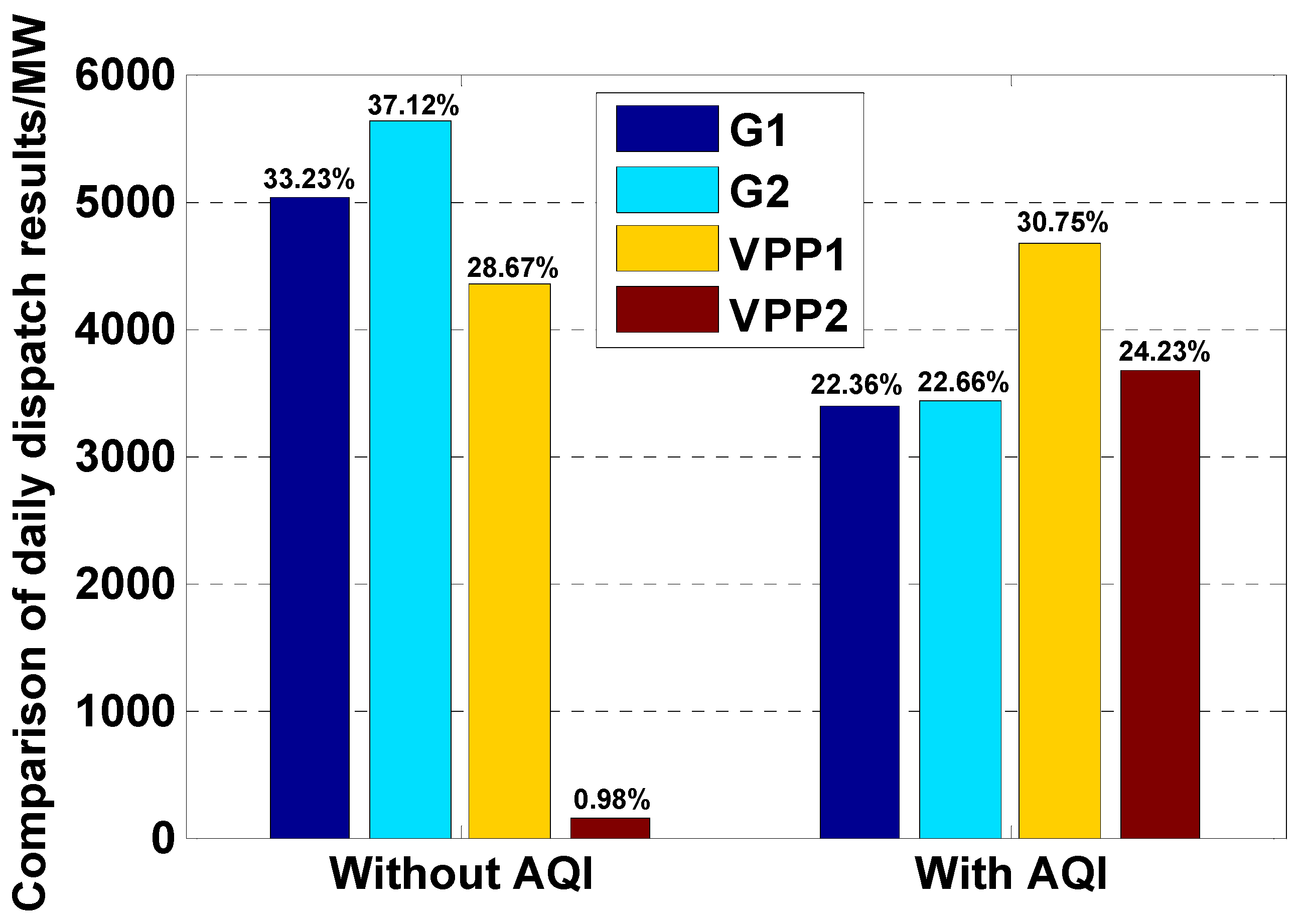
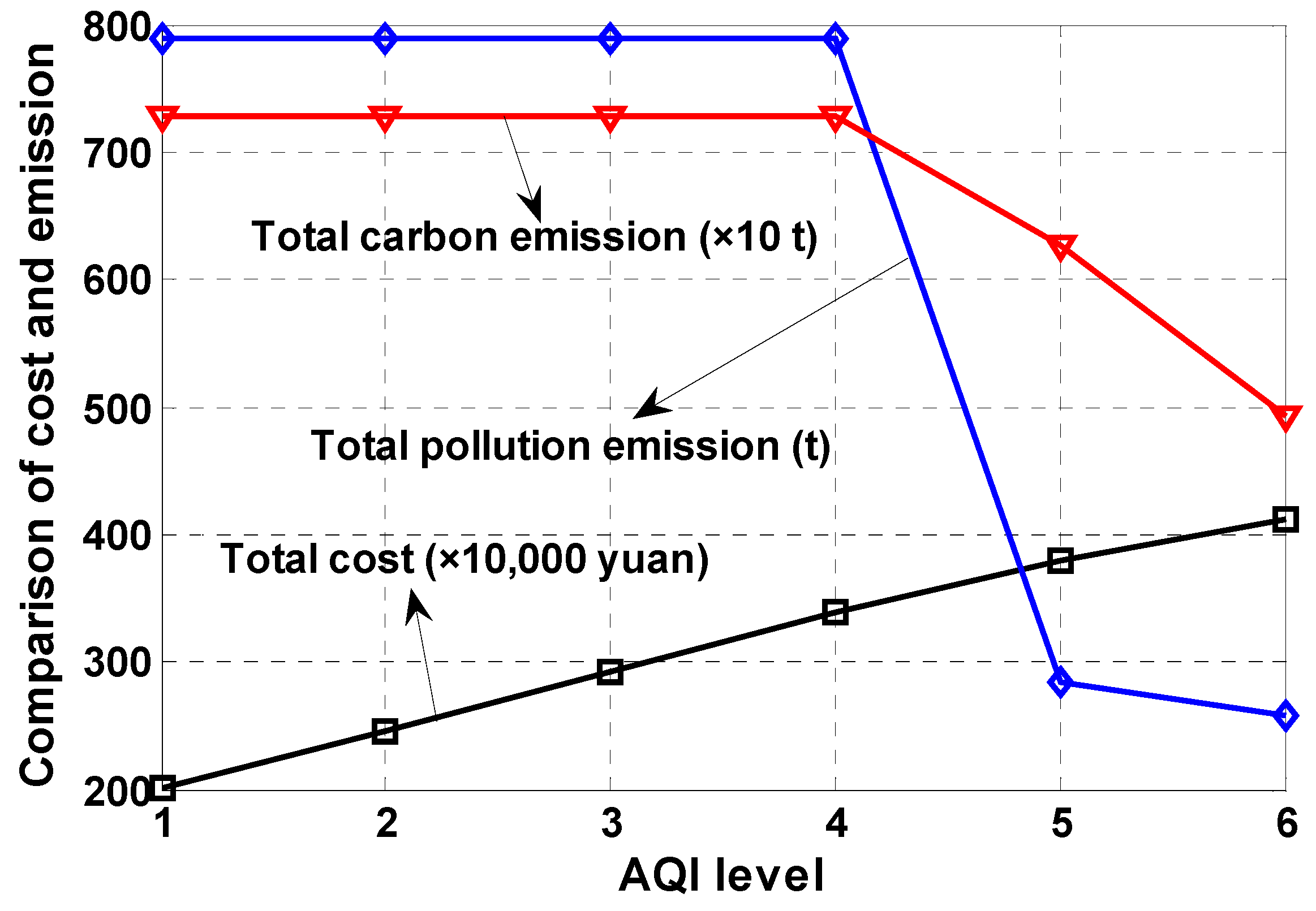
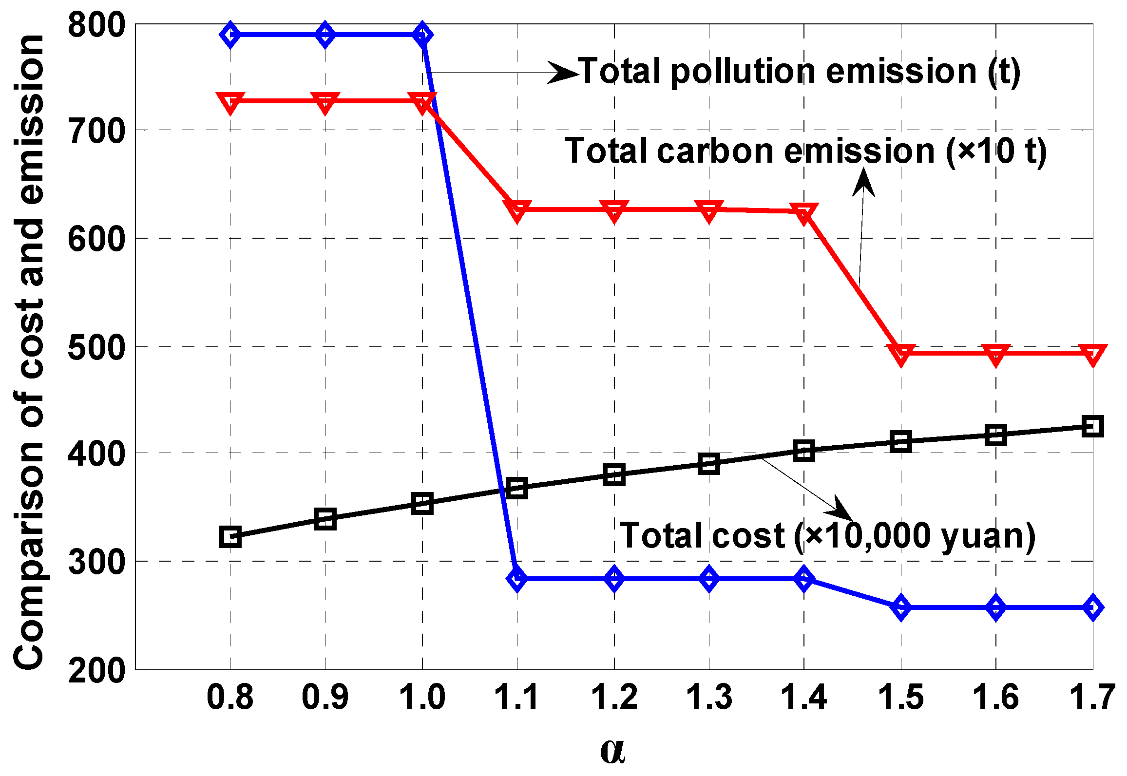
6.2. The Dispatch under F-H Weather
| Unit | aQi yuan/MW2 | bQi yuan/MW | cQi yuan | aWi kg/MW2 | bWi kg/MW | cWi kg |
|---|---|---|---|---|---|---|
| G1 | 0.018 | 38.306 | 1243.531 | 3.380 | −3.550 | 5.426 |
| G2 | 0.011 | 36.328 | 1658.570 | 6.490 | −5.554 | 5.090 |
| Unit | Pmin-Gi MW | Pmax-Gi MW | eGi t/MW | cei t/t | CBi yuan/t | CXi yuan/t | CSUi yuan | CSDi yuan | Jmax-i |
|---|---|---|---|---|---|---|---|---|---|
| G1 | 35 | 210 | 0.350 | 1.6 | 21 | 13 | 330 | 110 | 5 |
| G2 | 130 | 325 | 0.340 | 1.8 | 16 | 14 | 430 | 140 | 4 |

7. Conclusions
Acknowledgments
Author Contributions
Conflicts of Interest
References
- Zhang, X.D.; Liang, J. From London to Beijing: A comparison and reflexion on smog controls in China and Britain. Frontiers 2014, 2, 52–63. [Google Scholar]
- Cheng, W.L.; Kuo, Y.C.; Lin, P.L.; Chang, K.-H.; Chen, Y.-S.; Lin, T.-M.; Huang, R. Revised air quality index derived from an entropy function. Atmos. Environ. 2004, 38, 383–391. [Google Scholar] [CrossRef]
- Walling, R.A.; Saint, R.; Dugan, R.C.; Burke, J.; Kojovic, L.A. Summary of distributed resources impact on power delivery systems. IEEE Trans. Power Deliv. 2008, 23, 1636–1644. [Google Scholar] [CrossRef]
- Chaouachi, A.; Kamel, R.M.; Andoulsi, R.; Nagasaka, K. Multi objective intelligent energy management for a microgrid. IEEE Trans. Ind. Electron. 2013, 60, 1688–1699. [Google Scholar] [CrossRef]
- Chen, L.J.; Mei, S.W. An integrated control and protection system for photovoltaic microgrids. CSEE J. Power Energy Syst. 2015, 1, 36–42. [Google Scholar] [CrossRef]
- Mashhour, E.; Moghaddas, T.S. Bidding strategy of virtual power plant for participating in energy and spinning reserve markets-Part I: Problem formulation. IEEE Trans. Power Syst. 2011, 26, 949–956. [Google Scholar] [CrossRef]
- Giuntoli, M.; Poli, D. Optimized thermal and electrical scheduling of a large scale virtual power plant in the presence of energy storages. IEEE Trans. Smart Grid 2013, 22, 765–771. [Google Scholar] [CrossRef]
- Lu, Z.X.; Ye, X.; Qiao, Y.; Min, Y. Initial exploration of wind farm cluster hierarchical coordinated dispatch based on virtual power generator concept. CSEE J. Power Energy Syst. 2015, 1, 62–67. [Google Scholar] [CrossRef]
- Arslan, O.; Karasan, O.E. Cost and emission impacts of virtual power plant formation in plug-in hybrid electric vehicle penetrated networks. Energy 2013, 60, 116–124. [Google Scholar] [CrossRef]
- Vasirani, M.; Kota, R.; Cavalcante, R.L.G.; Ossowski, S.; Jennings, N.R. An agent-based approach to virtual power plants of wind power generators and electric vehicles. IEEE Trans. Smart Grid 2013, 4, 1314–1322. [Google Scholar] [CrossRef]
- Wille, H.B.; Erge, T.; Wittwer, C. Decentralized optimization of a cogeneration in virtual power plants. Sol. Energy 2010, 84, 604–601. [Google Scholar] [CrossRef]
- Wan, C.; Zhao, J.; Song, Y.H.; Xu, Z.; Lin, J.; Hu, Z.C. Photovoltaic and Solar Power Forecasting for Smart Grid Energy Management. CSEE J. Power Energy Syst. 2015, 1, 38–46. [Google Scholar] [CrossRef]
- Kang, C.Q.; Zhou, A.S.; Wang, P.; Zheng, G.; Liu, Y. Impact analysis of hourly weather factors in short-term load forecasting and its processing strategy. Power Syst. Technol. 2006, 30, 5–10. [Google Scholar]
- Nobre, A.M.; Karthik, S.; Liu, H.; Yang, D.; Martins, F.R.; Pereira, E.B.; Rüther, R.; Reindl, T.; Peters, I.M. On the impact of haze on the yield of photovoltaic systems in Singapore. Renew. Energy 2016, 89, 389–400. [Google Scholar] [CrossRef]
- Li, J.; Gao, Y.J.; Liu, J.P.; Ji, W.; Wang, N. The research of grid short-term load forecasting considering with air quality index. In Proceedings of the 2014 International Conference on Power System Technology (POWERCON 2014), Chengdu, China, 22–24 October 2014; pp. 852–857.
- Stock, J.H.; Watson, M.W. Forecasting using principal components from a large number of predictors. J. Am. Stat. Assoc. 2002, 97, 1167–1179. [Google Scholar] [CrossRef]
- Jin, M.; Zhou, X.; Zhang, Z.M.; Tentzeris, M.M. Short-term power load forecasting using grey correlation contest modeling. Expert Syst. Appl. 2012, 39, 773–779. [Google Scholar] [CrossRef]
- Beccali, M.; Cellura, M.; Brano, V.L.; Marvuglia, A. Forecasting daily urban electric load profiles using artificial neural networks. Energy Convers. Manag. 2004, 45, 2879–2900. [Google Scholar] [CrossRef]
- Hippert, H.S.; Pedreira, C.E.; Souza, R.C. Neural networks for short-term load forecasting: A review and evaluation. IEEE Trans. Power Syst. 2001, 16, 44–55. [Google Scholar] [CrossRef]
- Mandal, P.; Madhira, S.T.S.; Meng, J.; Pineda, R.L. Forecasting power output of solar photovoltaic system using wavelet transform and artificial intelligence techniques. Procedia Comput. Sci. 2012, 12, 332–337. [Google Scholar] [CrossRef]
- Chen, Y.; Luh, P.B.; Guan, C.; Zhao, Y.; Michel, L.D.; Coolbeth, M.A.; Friedland, P.B.; Rourke, S.J. Short-term load forecasting: Similar day-based wavelet neural networks. IEEE Trans. Power Syst. 2010, 25, 322–330. [Google Scholar] [CrossRef]
- Gao, Y.J.; Liu, D.; Cheng, H.X.; Tian, L.; Peng, L. State Key Laboratory of Alternate Electrical Power System With Renewable Energy Sources. Predictor-Corrector Model of Wind Power Forecast Based on Data-driven. Proc. CSEE 2015, 35, 2645–2653. [Google Scholar]
- Cheng, H.X.; Gao, Y.J.; Zhang, J.; Li, R.; Liang, H. The power system multi-objective optimization dispatching containing virtual power plant. In Proceedings of the 2014 International Conference on Power System Technology (POWERCON 2014), Chengdu, China, 22–24 October 2014; pp. 3316–3321.
- Viana, A.; Pedroso, J.P. A new MILP-based approach for unit commitment in power production planning. Int. J. Electr. Power Energy Syst. 2013, 44, 997–1005. [Google Scholar] [CrossRef]
- Carrión, M.; Arroyo, J.M. A computationally efficient mixed-integer linear formulation for the thermal unit commitment problem. IEEE Trans. Power Syst. 2006, 21, 1371–1378. [Google Scholar] [CrossRef]
- Xing, H.J.; Cheng, H.Z.; Zhang, L.B. Demand Response Based and Wind Farm Integrated Economic Dispatch. CSEE J. Power Energy Syst. 2015, 1, 47–51. [Google Scholar] [CrossRef]
- Gao, Y.J.; Liu, J.P.; Yang, J.; Liang, H.; Zhang, J. Multi-Objective Planning of Multi-Type Distributed Generation Considering Timing Characteristics and Environmental Benefits. Energies 2014, 7, 6242–6257. [Google Scholar] [CrossRef]
- Marler, R.T.; Arora, J.S. The weighted sum method for multi-objective optimization: New insights. Struct. Multidiscip. Optim. 2010, 41, 853–862. [Google Scholar] [CrossRef]
- Li, H.Z.; Wang, B.; Guo, S. Analytic Model and Benefits Measurement of Efficiency Power Plant Participating in Market Bidding Transaction in Smart Grid Environment. Power Syst. Technol. 2012, 36, 111–116. [Google Scholar]
- Liu, Z.P.; Wen, F.S.; Ledwich, G. Optimal planning of electric-vehicle charging stations in distribution systems. IEEE Trans. Power Deliv. 2013, 28, 102–110. [Google Scholar] [CrossRef]
- Yin, X.; Chen, W.Y. Cost of Carbon capture and storage and renewable energy generation based on the learning curve method. J. Tsinghua Univ. (Sci. Technol.) 2012, 52, 243–248. [Google Scholar]
© 2016 by the authors; licensee MDPI, Basel, Switzerland. This article is an open access article distributed under the terms and conditions of the Creative Commons by Attribution (CC-BY) license (http://creativecommons.org/licenses/by/4.0/).
Share and Cite
Gao, Y.; Cheng, H.; Zhu, J.; Liang, H.; Li, P. The Optimal Dispatch of a Power System Containing Virtual Power Plants under Fog and Haze Weather. Sustainability 2016, 8, 71. https://doi.org/10.3390/su8010071
Gao Y, Cheng H, Zhu J, Liang H, Li P. The Optimal Dispatch of a Power System Containing Virtual Power Plants under Fog and Haze Weather. Sustainability. 2016; 8(1):71. https://doi.org/10.3390/su8010071
Chicago/Turabian StyleGao, Yajing, Huaxin Cheng, Jing Zhu, Haifeng Liang, and Peng Li. 2016. "The Optimal Dispatch of a Power System Containing Virtual Power Plants under Fog and Haze Weather" Sustainability 8, no. 1: 71. https://doi.org/10.3390/su8010071
APA StyleGao, Y., Cheng, H., Zhu, J., Liang, H., & Li, P. (2016). The Optimal Dispatch of a Power System Containing Virtual Power Plants under Fog and Haze Weather. Sustainability, 8(1), 71. https://doi.org/10.3390/su8010071