Stochastic Pricing and Order Model with Transportation Mode Selection for Low-Carbon Retailers

Abstract

More and more enterprises have begun to pay attention to their carbon footprint in the supply chain, of which transportation has become the second major source of carbon emissions. This paper aims to study both optimum pricing and order quantities, considering consumer demand and the selection of transportation modes by retailers, in terms of carbon emissions sensitivity and price sensitivity under the conditions of a cap-and-trade policy and uncertain market demand. Firstly, we analyze the effects of transportation mode (including transportation costs and transportation-induced carbon emissions), initial emissions allowances, carbon emissions trading price and consumer sensitivity to carbon emissions on the optimum decisions and profits of retailers. The results demonstrate that when consumers are less sensitive to price, the optimum retail price and the optimum order quantity of products are proportional to the transportation cost and transportation-induced carbon emissions of retailers per unit product, the carbon emissions trading price as well as consumer sensitivity to carbon emissions. However, when consumers are highly sensitive to price, the optimum order quantity of products is inversely proportional to the transportation costs and transportation-induced carbon emissions of retailers per unit product, the carbon emissions trading price and consumer sensitivity to carbon emissions. In addition, the optimum retail price of products is inversely proportional to consumer sensitivity to carbon emissions. We also find that retailers prefer a low-carbon transportation mode when the carbon emissions trading price is high. Meanwhile, the carbon emissions trading price influences the carbon emissions trading volume of retailers. These theoretical findings are further validated by some numerical analysis.

1. Introduction

With the rapid development of the modern economy, the frequency of transport of production materials and finished goods has grown tremendously, which opens up great opportunities for the development of global logistics. However, continual climate change has attracted increasing concern from scientists, entrepreneurs and the public [1]. Promoting a green, low-carbon economy has become an important task in the current readjustment of the world economic structure. Transportation, an important carrier and tool of economic and social development, is the lifeline of economic development of a country. Cristea et al. suggested freight transport growth and energy consumption growth will lead to a similar increase in transport carbon emissions [2]. Transportation has the highest energy consumption and the quickest energy consumption growth, and is viewed as an important source of greenhouse gas. Therefore, the increase in transport frequency, carbon emissions and energy consumption will put huge pressure on the environment [3,4]. Transportation will cause serious environmental pollution, global warming and frequent natural disasters. Moreover, the emission of tremendous tail gas will further intensify haze phenomena around the whole world and threaten human health. As it was reported by the International Energy Agency (IEA) in 2009, about 25% of carbon dioxide emissions in the world come from transportation, while 50% of atmospheric pollution in the United States and 20% of carbon emissions in Japan are caused by transportation. The Asian Development Bank predicted that global carbon dioxide emissions caused by transportation will increase by 57% over a period of 25 years, and the energy consumption by global transportation will be doubled in 2050 [5]. In such cases, selecting a high-efficiency and low-emission transportation mode becomes extremely important.

In recent times, due to increasing environmental concern and change in consumers’ habits, consumers have been willing to pay more for green, low-carbon products [6]. According to a survey of the European Commission, 83% of Europeans pay great attention to the environmental impact of products when making purchases. Additionally, the environmental protection awareness of consumers drives enterprises in the supply chain to adopt low-carbon practices to win more customers [7]. The low-carbon preference of consumers and the low-carbon policies of government will surely significantly influence the business and production modes of enterprises as well as the competition and cooperation between enterprises [8]. The Congressional Budget Office (CBO) of the Congress of the United States [9] provided a comprehensive study on the policy options for reducing CO₂ emissions and furnished four major carbon emissions policies as follows: (i) a mandatory capacity for the amount of carbon emitted by each firm; (ii) a tax imposed to each firm for the amount of carbon emissions; (iii) a cap-and-trade system implemented to allow emissions trading; and (iv) an investment made by each firm in carbon offsets to meet its carbon capacity requirement. The carbon cap-and-trade policy could play an important role in both administrative control and the market. It has been regarded as the most effective emissions reduction method and is the first choice of national governments [10].

In decision-making regarding transportation problems, the transportation mode is the first consideration of enterprises. Nevertheless, common transportation modes, such as railway transportation, highway transportation, shipment and air transportation, have unique advantages in terms of transportation costs, mean transport time, transportation capacity, accessibility and security. They are difficult to measure using a uniform index. Taking into consideration government policy regarding carbon emissions and consumers’ sensitivity to carbon emissions, this paper evaluates transportation modes in terms of transportation costs and transportation-induced carbon emissions per unit product with uncertain market demand. On this basis, we can obtain an optimal combined strategy that incorporates transportation mode, retail price and order quantity. This paper mainly focuses on the following two problems:

(1)

Under the carbon cap-and-trade policy and high consumer sensitivity to carbon emission, how retailers choose their transportation mode, pricing strategy and order strategy while promising the maximum profit.

(2)

Effect of transportation mode (transportation cost per unit product and transportation-induced carbon emission per unit product), carbon emissions policy (initial emission allowances and carbon emission trading price) and consumers’ sensitivity to carbon emissions on the optimum pricing, optimum order quantity and the maximum expected profit of the retailer.

To solve these problems, we firstly discussed how a monopoly retailer who wants to achieve the maximum profit makes decisions about the optimum transportation mode, the optimum pricing and the optimum order quantity under the influence of consumer sensitivity to carbon emissions and price. Next, the effect of transportation mode, carbon emissions policy and consumer sensitivity on the optimum decision-making and maximum profit of retailers is analyzed. Finally, the model conclusions are validated through numerical analysis. This paper uses the transportation cost and cost for transportation-induced carbon emissions as the general cost to select the transportation mode. It extends the decision-making model of retailer transportation selection and expands carbon emission policy as well as consumer sensitivity demands into the research scope of retailers. The results of this paper can provide references for governments to make policy on carbon emissions and provide retailers support in decision making for energy saving and emissions reduction, low-carbon transportation selection and low-carbon operation management.

Based on these objectives, the remainder of this paper is set out as follows: Section 2 is a literature review. Section 3 is a problem description and related assumptions. Section 4 introduces decision-making on the optimal pricing, optimum order and optimum transportation mode of retailers. Section 5 analyzes sensitivity of related parameters to the optimum decision-making of retailers. Section 6 is a numerical analysis based on specific cases to verify model results. Section 7 is the conclusion and future research directions.

2. Literature Review

Many achievements in low-carbon operation management have been reported in recent years. Benjaafar et al. [11] introduced the idea of carbon emissions constraints in the supply chain system. They studied purchase, production, inventory and green technology investment strategies under the carbon cap-and-trade policy, and analyzed the effect of cooperation of enterprises in the supply chain on operating costs and carbon emissions reduction. Song and Leng [12] explored the typical single-period problem under different carbon emissions policies and determined the optimum production of enterprises under each policy as well as corresponding expected profits. Zhao et al. [13] studied carbon reduction decisions of enterprises in the supply chain in response to low-carbon policy, and established a Stackeberg game model dominated by manufacturers, to obtain the optimum emissions reduction scenario and determine the optimum production of enterprises. Diabat et al. [14] examined the carbon emissions in production, inventory and delivery, and analyzed the effect of different carbon emissions policies on the economic performance of the supply chain. Based on a supply chain composed of one supplier with carbon emissions license and one enterprise with carbon emissions dependence, Du et al. [15] studied the effect of a carbon cap-and-trade mechanism on decision-making of different supply chain members under the framework of a Newsvendor model and obtained the sole Nash equilibrium solution. Wahab et al. [16] constructed a supply chain composed of one supplier and one retailer. They established an economic order quantity (EOQ) model to find the minimum cost under the carbon cap-and-trade policy, and determined the optimum order strategy for the retailer. Yang et al. [17] studied an equilibrium model of supply chain for the power sector, getting the optimum burning energy and the optimum carbon emissions of fuels. These studies take carbon emissions polices into account, but neglect consumers’ carbon-sensitive demands. Purohit and Shankar et al. [18,19] develop an integer linear programming model to discuss the inventory lot-sizing problem under non-stationary stochastic demand conditions with emissions and cycle service level constraints, considering a carbon cap-and-trade policy.

Conrad [20] established an oligopoly model within the consumer context, which was used to decide price, product features and market competition of enterprises. Liu et al. [21] discussed horizontal competition between manufacturers and retailers in three different supply chain structures under the influence of consumer carbon-sensitive demand. They found that the increasing environmental consciousness of consumers could improve the optimum decision-making in the operations of both retailers and manufacturers. Nouira et al. [22] studied the optimum production system of manufacturing enterprises with consideration given to consumer carbon-sensitive demand. They believed that attention must be paid to the effect of carbon emissions during work flow design and raw material input on the environment. Additionally, they discussed the impact of consumer carbon-sensitive demand on profit and decision-making of manufacturing enterprises.

The retailer is an important component of the supply chain. The transportation mode selected by retailers plays an extremely important role in the low-carbon footprint of the whole supply chain. For transportation route selection, Chang [23] established a multi-objective optimization model considering multiple commodity flows for the multimodal transport path route selection. Time constraints, transportation mode selection and transportation costs were considered in this model. Liao [24,25] calculated carbon dioxide emissions of inland container transportation from 1998 to 2008 in Taiwan, and predicted the variation trend of carbon emissions. On this basis, he also discussed carbon dioxide emissions of highway transportation and multimodal transport. Goel [26] proved that the general cargo dead weight, routing selection and on-travel visibility in the multimodal transport network model could be used to adjust transportation planning and traffic operation systems. The experimental research confirmed that these conditions could increase delivery punctuality. This model is applicable in building green standards, such as carbon emission standards, energy consumption standards, food spoilage and loss standards, etc. To evaluate the effect on society and the environment, Janic [27] transformed a large airport into a real multimodal transport node. This means integrating the airport into a surrounding high-speed railway network and regarding some short-distance air passenger transportation modes as equal to high-speed railway transportation services. With respect to transportation mode, Mckinnon [28] concluded through an empirical study that structure, business, operation, function and external factors are the most important connected factors that influence carbon dioxide emissions in highway transportation. Only few researches viewed transportation mode as a decision variable. With consideration given to economic value and the social environment, Leal and D’Agosto [29] obtained an alternative transportation mode for ethyl alcohol through modeling. They found that the combination of local highway transportation and direct delivery to the end port of ethyl alcohol by injecting it into a long-distance pipeline is the best transportation mode. Cholatte and Venkat [30] studied wine transportation in California according to the distance between consumers. They considered varied network planning and design approaches in the wine supply chain, examining carbon emissions during travel, and developed an inventory of every transportation node, finding that the transportation mode could significantly affect the carbon emissions in the whole supply chain. These two researchers studied decision-making regarding transportation modes based on specific cases, but did not establish a universal supply chain model for discussion. Hoen [31,32] was the first one who studied universal transportation mode selection. He pointed out that the carbon emission of retailers could be reduced by adjusting different transportation modes. Firstly, the actual carbon emission data of different transportation modes selected by retailers were measured. The empirical analysis revealed that adjusting transportation mode could reduce carbon emissions by 10% with only a logistics cost increase of 0.7%. Retailers could form strategies according to practical situations. All of these researches did not involve retailers’ decision-making for transportation mode selection from the perspective of consumers’ carbon-sensitive demands when enterprises were restricted by carbon emissions policies. To solve these problems, based on an uncertain market, in the following, we shall study decision-making regarding optimum transportation mode, pricing and order quantity of retailers with consideration given to consumers’ carbon-sensitive demands and the carbon cap-and-trade policy.

3. Problem Description and Assumptions

To facilitate the discussion, in this section, we describe the research problem as well as some assumptions.

Suppose a monopoly retailer of a seasonal product is taken as the object in this paper. Faced with uncertain market demand, this retailer purchases a product at the wholesale price of $\omega$ and sells it to consumers who are sensitive to both price and carbon emissions per unit. Consumers could observe carbon emissions per product during transportation directly in some way (e.g., carbon footprint and green product certification). Consumer demand is negatively correlated with carbon emissions in transportation per unit product $e$ and the unit retail price $p$. The demand function is as follows:

$$D\left(p,e,\epsilon \right)=\alpha -\beta p-\gamma e+\epsilon ,\epsilon \in \left[A,B\right]$$

(1)

where $\mathsf{\alpha }$, $\mathsf{\beta }$ and $\mathsf{\gamma }$ represent market attributes of consumers: $\mathsf{\alpha }$ is market size; $\mathsf{\beta }$ is market sensitivity to retail price of the product; $\mathsf{\gamma }$ is market sensitivity to carbon emission per unit product; $\epsilon$ is a random variable and expresses random fluctuation of product demand, whose value is from A to B; $f(·)$ is probability density function of random demand; $F(·)$ is the distribution function of random demand.

Under a carbon cap-and-trade policy, the initial emission allowances to the retailer within a single-period is $E_0$. If the carbon emission of the retailer within a single-period $E_q$ is smaller than $E_0$, he could sell residual carbon emissions permit at a price of $C_e$ in the carbon emissions trading market. On the contrary, he needs to buy extra carbon emissions permit from the carbon emissions trading market at the same price $C_e$. Due to the uncertain market demand, in a situation of oversupply, surplus products could be sold at a discount $v$, but under supply shortage, the retailer has to pay for shortage costs $s$ as a penalty. The Parameters and variables in this paper are shown in Table 1.

Table 1. Parameters and variables.

Notation	Descriptions
$q$	Ordering quantity or customer demands of retailer.
$p$	Unit retail price of retailer.
$E_0$	Initial carbon emission allowances from government.
$e_1$, $e_2$	Unit carbon emissions of transport mode 1 and 2, respectively, $e_1<e_2$
$c_1$, $c_2$	Unit transportation cost of transport mode 1 and 2, respectively, $c_1>c_2$
$e$	Unit carbon emission quantity of products.
$C_e$	Unit price of carbon emission trading.
$\lambda$	Transportation proportion part of transportation mode 1 $0\le \lambda \le 1$.
$\epsilon$	Random variable
$w$	Unit procurement cost of product.
$s$	Unit Shortage cost of product.
$v$	Unit Salvage value of product.
$\alpha$	Initial market potential.
$\beta$	Coefficient of retail price impact on demand.
$\gamma$	Coefficient of carbon emission impact on demand.
$\pi$	Profit of retailer.

Table 1. Parameters and variables.

Notation	Descriptions
$q$	Ordering quantity or customer demands of retailer.
$p$	Unit retail price of retailer.
$E_0$	Initial carbon emission allowances from government.
$e_1$, $e_2$	Unit carbon emissions of transport mode 1 and 2, respectively, $e_1<e_2$
$c_1$, $c_2$	Unit transportation cost of transport mode 1 and 2, respectively, $c_1>c_2$
$e$	Unit carbon emission quantity of products.
$C_e$	Unit price of carbon emission trading.
$\lambda$	Transportation proportion part of transportation mode 1 $0\le \lambda \le 1$.
$\epsilon$	Random variable
$w$	Unit procurement cost of product.
$s$	Unit Shortage cost of product.
$v$	Unit Salvage value of product.
$\alpha$	Initial market potential.
$\beta$	Coefficient of retail price impact on demand.
$\gamma$	Coefficient of carbon emission impact on demand.
$\pi$	Profit of retailer.

To ensure the established model has practical significance, this paper has some assumptions:

• $p>\omega >s>v$. This implies that the retailer could achieve profit growth by selling the product.
• Carbon emissions of product not only exist in transportation to the retailer, but also exist in production. We assume that manufacturer’s technological level should remain unchanged, then carbon emissions in production will remain the same, so α in Equation (1) denotes the effect of carbon emissions in production on consumer demand. Different transportation modes have different transportation costs and carbon emissions per unit product. Taking railway transportation and shipment for example: shipment has a lower transportation cost per unit product but higher carbon emissions per unit product, while railway transportation shows the opposite.
• There are two alternative transportation modes (named as Mode 1 and Mode 2) for the retailer: $c_1$ and $c_2$ represent transportation costs of Mode 1 and Mode 2, respectively; $e_1$ and $e_2$ represent carbon emissions of Mode 1 and Mode 2, respectively. If $c_1>c_2$ and ${\mathrm{e}}_1<{\mathrm{e}}_2$, this condition means that Mode 1 has higher unit transportation cost and higher unit transportation carbon emissions than that of Mode 2, so Mode 2 is the better transportation mode obviously. Likewise, if $c_1<c_2$ and $e_1<e_2$, Mode 1 is the better transportation mode obviously. So, in the following context, we assume that $c_1>c_2$ and $e_1<e_2$ to study the potential rules governing retailers’ strategies. This assumption also holds in reality. For example, considering the two different transport modes—railway transportation and shipping transportation—the train transportation cost is higher than the cost of shipping transportation $c_1>c_2$, but the shipping transportation carbon emissions is higher than the transportation carbon emissions of railway transportation, i.e., $e_1<e_2$. Such an assumption also can be found in [33,34]. We assume that the quantity of the retailer’s products for transportation is enough to meet the economies of scale.

Let $\lambda \left(\lambda \in [0, 1]\right)$ represent the selection proportion for transport Mode 1 of the transport quantities, Then, $1-\lambda$ is the selection proportion of transport Mode 2 of the transport quantities. On this basis, the general transportation cost $c(\lambda )$ and the general transportation-induced carbon emissions $e(\lambda )$ per unit product of the retailer could be calculated:

$$c(\lambda )=\lambda c_1+\left(1-\lambda \right)c_2$$

(2)

$$e(\lambda )=\lambda e_1+\left(1-\lambda \right)e_2$$

(3)

The retailer’s decision regarding transportation mode could be converted into a decision about $\lambda$. When $\lambda =1$, the retailer will apply Mode 1 to all products. When $\lambda =0$, the retailer will apply Mode 2 to all products. When $0<\lambda <1$, the retailer will apply both Mode 1 and Mode 2.

Based on the above hypotheses and analysis, this paper establishes a classical Newsvendor model, and the profit function of the retailer is as follows:

$$\pi \left(q,p,\lambda \right)=p\times min\left\{D\left(p,\lambda ,\epsilon \right),q\right\}-c\left(\lambda \right)q-\omega q+v{\left[q-D\left(p,\lambda ,\epsilon \right)\right]}^{+}-s{\left[D\left(p,\lambda ,\epsilon \right)-q\right]}^{+}-C_e\left[e\left(\lambda \right)q-E_0\right]$$

where $p\times min\left\{D\left(p,\lambda ,\epsilon \right),q\right\}$ is the sales revenue of the retailer; $c\left(\lambda \right)q$, $\omega q$, $s{\left[D\left(p,\lambda ,\epsilon \right)-q\right]}^{+}$ are the transportation cost, the ordering cost and the shortage cost, respectively; $v{\left[q-D\left(p,\lambda ,\epsilon \right)\right]}^{+}$ is the revenue of slow seller at the end of the marketing season; $e\left(\lambda \right)q-E_0=E_q$ is the carbon emissions during production transportation to the retailer under the carbon cap-and-trade policy. If $E_q<0$, the retailer has a surplus carbon emissions permit which could be sold in the carbon emissions trading market; otherwise, the retailer has to buy an extra carbon emissions permit from the carbon emissions trading market.

Let $C_{\lambda }=C_{e}e\left(\lambda \right)+c\left(\lambda \right)+\omega$ represent the general selling cost per unit product. Then,

$$\pi \left(q,p,\lambda \right)=p\times min\left\{D\left(p,\lambda ,\epsilon \right),q\right\}-C_{\lambda }q+v{\left[q-D\left(p,\lambda ,\epsilon \right)\right]}^{+}-s{\left[D\left(p,\lambda ,\epsilon \right)-q\right]}^{+}+C_e{E}_0$$

(4)

Motivated by the operation idea in the reference of Petruzi and Dada [35], let $g\left(p,\lambda \right)=\alpha -\beta p-\gamma e\left(\lambda \right)$ represent the consumer demand of the product. We define $z=q-g\left(p,\lambda \right)$, $z\in \left[A,B\right]$ to express the inventory factor of the retailer: when $z>0$, the retailer owns surplus products, known as surplus inventory; when $z<0$, the retailer does not have adequate products to meet consumer demand. Hence, the decision problem with respect to $q,p,\lambda$ is equivalent to the decision problem with respect to $z,p,\lambda$. This conversion will not affect the retailer’s optimal decision, just for the sake of more convenient calculation. Let $F(·)$ be the distribution function of $\epsilon$, f($·$) be the probability density function of $\epsilon$, and $F\left(A\right)=0, F\left(B\right)=1$. Then, the expected profit of the retailer is:

$$E\left[\pi \left(z,p,\lambda \right)\right]=p{{\displaystyle \int }}_A^z\left(u-z\right)f\left(u\right)du+v{{\displaystyle \int }}_A^z\left(z-u\right)f\left(u\right)du-s{{\displaystyle \int }}_z^B\left(u-z\right)f\left(u\right)du+\left(p-C_{\lambda }\right)\left[z+g\left(p,\lambda \right)\right]+C_e{E}_0$$

4. The Optimal Decision Making Models for the Retailer

To make an optimal decision, the retailer should firstly calculate the optimum retail price $p^{*}$ and the optimum order quantity $q^{*}$ (or $z^{*}$) after the transportation mode is determined. Both of them are response functions about the transportation mode, shown as, $p^{*}=p\left(\mathsf{\lambda }\right)$, $q^{*}=q\left(\mathsf{\lambda }\right)$, $z^{*}=z\left(\mathsf{\lambda }\right)$. Next, substitute the optimal decision under the determined transportation mode into the expected profit of the retailer. The optimum transportation mode for achieving the maximum expected profit of the retailer is ${\lambda }^{*}$:

$$E\left[\pi \left(p,z\right)\right]=p{{\displaystyle \int }}_A^z\left(u-z\right)f\left(u\right)du+v{{\displaystyle \int }}_A^z\left(z-u\right)f\left(u\right)du-s{{\displaystyle \int }}_z^B\left(u-z\right)f\left(u\right)du+\left(p-C_{\lambda }\right)\left[z+g\left(p,\lambda \right)\right]+C_e{E}_0$$

(5)

Lemma 1. 

After the transportation mode is selected, for a given $z$, the optimum retail price is $p^{*}=p\left(z\right)=p_0-\frac{{{\displaystyle \int }}_z^B\left(u-z\right)f\left(u\right)du}{2\beta }$.

Lemma 2. 

Under the determined transportation mode, $q^{*}=z^{*}+g\left( p^{*},\lambda \right)$, $p^{*}=p\left(z^{*}\right)$, where $z^{*}$ is determined by the following conditions:

(1) 

For an arbitrary distribution function $F\left(z\right)$, the retailer could find the optimal value$z^{*}$ within the interval $z\in \left[A,B\right]$.

(2) 

For the distribution function$F\left(z\right)$, if $z^{*}$ meets $f^2\left(z\right)+f^{\text{'}}\left(z\right)\left[1-F\left(z\right)\right]>0$ within the interval $A\le z\le B$, $z^{*}$ is the maximum one satisfying $\frac{\partial E\left[\pi \left(p,z\right)\right]}{\partial z}=0$.

(3) 

When (2) and$A>\beta \left(C_{\lambda }-2s\right)-\alpha +\gamma e\left(\lambda \right)$ are met, $z^{*}$ is the sole solution meeting $\frac{\partial E\left[\pi \left(p,z\right)\right]}{\partial z}=0$ in the interval$A\le z\le B$.

The Proofs of Lemma 1 and Lemma 2 are provided in the Appendix.

Lemma 1 and Lemma 2 indicate that we can calculate the optimum retail price $p^{*}$ and the optimum order quantity $q^{*}$ of the product, which are both related to the transportation mode $\lambda$. Then, with Equation (5), we can obtain the optimum transportation mode ${\mathsf{\lambda }}^{*}$ of the retailer:

$$E\left[\pi \left(\lambda \right)\right]=p^{*}{{\displaystyle \int }}_A^{z^{*}}\left(u-z^{*}\right)f\left(u\right)du+v{{\displaystyle \int }}_A^{z^{*}}\left(z^{*}-u\right)f\left(u\right)du-s{{\displaystyle \int }}_{z^{*}}^B\left(u-z^{*}\right)f\left(u\right)du+\left(p^{*}-C_{\lambda }\right)\left[z^{*}+g\left(p^{*},\lambda \right)\right]+C_e{E}_0$$

(6)

This, together with Lemma 1, allows us to obtain the following theorem. The Proof of Theorem 1 is provided in the Appendix.

Theorem 1. 

The optimal transportation mode for the retailer (${\lambda }^{*}$) is decided by the carbon trade price $C_e$:

(1) 

If$C_e\ge \frac{c_1-c_2}{e_2-e_1}$, $E\left[\pi \left(\lambda \right)\right]$ is a strictly increasing convex function of$\lambda$, then${\lambda }^{*}=1$.

(2) 

If$C_e<\frac{c_1-c_2}{e_2-e_1}$, $E\left[\pi \left(\lambda \right)\right]$ is a concave function of$\lambda$, that is,${\lambda }^{*}$ is decided by the place of$\frac{dE\left[\pi \left(\lambda \right)\right]}{d\lambda }$=0; We set the place of$\frac{dE\left[\pi \left(\lambda \right)\right]}{d\lambda }$=0 is a, if$a\in \left(0,1\right)$, then$\frac{dE\left[\pi \left[p^{*}\left(z^{*}\left(\lambda \right),\lambda \right),z^{*}\left(\lambda \right),\lambda \right]\right]}{d\lambda }=0{|}_{\lambda ={\lambda }^{*}}$. If$a>1$, then${\lambda }^{*}=1$. If$a<0$, then${\lambda }^{*}=0$.

Theorem 1 reveals that the optimum transportation mode is determined by the carbon emissions trading price. When the carbon emissions trading price is $C_e\ge \frac{c_1-c_2}{e_2-e_1}$, the effect of carbon emissions cost during transportation on profit of the retailer is always larger than the effect of transportation cost. At this moment, the retailer will choose a transportation mode with low carbon emissions. When the carbon emissions trading price is $C_e<\frac{c_1-c_2}{e_2-e_1}$, the optimum transportation mode may not be the one with the minimum carbon emissions. Hence, to give full credence to the carbon cap-and-trade policy, the government shall adjust the carbon emissions trading price within $C_e\ge \frac{c_1-c_2}{e_2-e_1}$, so that it can drive retailers to pay attention to energy saving and emissions reduction and facilitate the development of low-carbon transportation.

5. Sensitivity Analysis

This section conducts a sensitivity analysis toward the optimal decision of the retailer. We analyze the effects of different parameter values of carbon cap-and-trade policy and transportation mode on the optimal decision and the maximum expected profit of the retailer. Firstly, the following theorem is yielded.

Theorem 2. 

When the transportation mode is determined (e.g., ${\lambda }^{*}=1，e\left({\lambda }^{*}\right)=e_1，c\left({\lambda }^{*}\right)=c_1$), let ${\beta }_0=\frac{{\left[1-F\left(z\right)\right]}^3}{2\left(c_1-v\right)f\left(z\right)}$:

(1) 

If$\beta <{\beta }_0, then \frac{d{p}^{*}}{d{c}_1}>0$, $\frac{d{q}^{*}}{d{c}_1}>0$； If$\beta >{\beta }_0,then \frac{d{q}^{*}}{d{c}_1}<0$.

(2) 

If$\beta <{\beta }_0$, $then \frac{d{p}^{*}}{d{e}_1}>0$, $\frac{d{q}^{*}}{d{e}_1}>0$； If$\beta >{\beta }_0$, then$\frac{d{q}^{*}}{d{e}_1}<0$.

The Proof of Theorem 2 is provided in the Appendix.

Theorem 2 demonstrates that when transportation costs or carbon emissions caused by transportation of the retailer change, the optimum order quantity and the sale price of the product will change accordingly. Such a variation trend is determined by consumer sensitivity to product price. When consumer sensitivity to product price is lower than the critical value, increasing transportation costs or carbon emissions will increase the retail price of a product and the order quantity. When consumer sensitivity to product price is higher than the critical value, increasing transportation costs or carbon emissions will decrease the order quantity of a retailer.

Under the carbon cap-and-trade policy, the government restricts retail transportation through the carbon emissions trading price and carbon caps. The following theorem reveals that the carbon emissions trading price could influence the order and pricing strategies of a retailer.

Theorem 3. 

If $\beta <{\beta }_0,then \frac{d{p}^{*}}{d{C}_e}>0,\frac{d{q}^{*}}{d{C}_e}>0$; if $\beta >{\beta }_0,then \frac{d{q}^{*}}{d{C}_e}<0$.

The Proof of Theorem 3 is provided in the Appendix.

Theorem 3 reflects that the change of the carbon emissions trading price will influence the optimum order quantity and the retail price of a product. Such degree of influence is also determined by consumer sensitivity to price. When consumer sensitivity to product price is higher than the critical value, increasing the carbon emissions trading price will reduce the order quantity of a retailer. However, when consumer sensitivity to product price is lower than the critical value, increasing the carbon emissions trading price will increase the order quantity and the retail price of a product.

Corollary 1. 

Under the conditions of a carbon cap-and-trade policy, if $\mathsf{\beta }<{\mathsf{\beta }}_0$, the retail price and order quantity of the product are higher than those under no restrictions of carbon emissions policy; If $\mathsf{\beta }>{\mathsf{\beta }}_0$, the order quantity of a product is less than that under no restrictions of carbon emissions policy.

The Proof of Corollary 1 is provided in the Appendix.

Theorem 4. 

$\frac{d{p}^{*}}{d{E}_0}=0$, $\frac{d{q}^{*}}{d{E}_0}=0, \frac{\partial E\left[\pi \left(p^{*},z^{*}\right)\right]}{\partial E_0}=C_e>0$.

The Proof of Theorem 4 is provided in the Appendix.

According to Theorem 4, the initial emission allowances do not influence the optimum order quantity and the optimum retail price of the retailer, but affect the expected profit of the retailer. The higher the initial emissions allowances, the higher the expected profit of the retailer. Moreover, the growth rate of profit is equal to the carbon emissions trading price.

The carbon cap-and-trade policy could adjust transportation mode selection, pricing and order behaviors of the retailer to a certain extent. Theorem 6 reveals the effect of consumer sensitivity to carbon emission on decision-making of the retailer.

Theorem 5. 

(1) If $\beta <{\beta }_0$, then $\frac{d{p}^{*}}{d\gamma }>0$, $\frac{d{q}^{*}}{d\gamma }>0$. If $\beta >{\beta }_0$, then$\frac{d{p}^{*}}{d\gamma }<0$, $\frac{d{q}^{*}}{d\gamma }<0$; (2) $\frac{dE\left[\pi \left(\gamma \right)\right]}{d\gamma }<0$.

The Proof of Theorem 5 is provided in the Appendix.

Theorem 5 indicates that consumers’ sensitivity to carbon emissions will influence the optimum order quantity and the optimum retail price. When consumer sensitivity to carbon emissions is smaller than the critical value, that is, consumers are less sensitive to price but are highly sensitive to carbon emissions, the retailer will raise retail price and increase the order quantity of the product. On the contrary, when consumers’ sensitivity to carbon emissions is higher than the critical value, that is, consumers are very sensitive to price, consumer sensitivity to carbon emissions is inversely proportional to retail price and order quantity of the product. The retailer has to lower the retail price in order to gain market share.

It can be deduced from Theorem 5 that when $\gamma >0$, consumers are sensitive to the carbon emissions of a product; when $\gamma =0$, consumers are insensitive to the carbon emissions of a product. Therefore, it can be inferred from Theorem 5 that when consumers are sensitive to carbon emissions of the product, retailer profit is lower than that when consumers are insensitive to carbon emissions. If $\beta <{\beta }_0$, the retail price and order quantity when consumers are sensitive to carbon emissions are higher than that when consumers are insensitive to carbon emissions. If $\beta >{\beta }_0$, the retail price and order quantity when consumers are sensitive to carbon emissions are lower.

6. Numerical Analysis

Based on above analysis, both carbon cap-and-trade policy and consumers’ carbon-sensitive demand will influence the optimal decision of the retailer. In this section, a typical case study is conducted to verify the theoretical findings of this paper.

Suppose there is a market demand$D\left(p,e\right)=200-2p-10e+\epsilon \left(\beta >{\beta }_0\right)$, where $\epsilon$ is a random variable which conforms to the uniform distributions [−50, 50], $F\left(-50\right)=0,F\left(50\right)=1$, $C_e=1$, $E_0=80$. For transportation mode 1, $c_1=2$, $e_1=1$. For transportation mode 2, $c_2=1.4$, $e_2=2$. $\omega =5$, $v=1$ and $s=2$. As it was introduced above, when $C_e\left(e_1-e_2\right)+\left(c_1-c_2\right)<0$, ${\lambda }^{*}=1$, the retailer prefers transportation mode 1 and thus $C_{\lambda }=C_1=C_{e}e\left(\lambda \right)+c\left(\lambda \right)+\omega =8$. The optimum retail price under no demand fluctuation is $p_0=51.5$ and the inventory parameter $z_1^{*}=36.6$, ${p_1}^{*}=51.3$, $q_1^{*}=z_1^{*}+\alpha -\beta {p_{\lambda }}^{*}-\gamma e\left(\lambda \right)=124$. At the same time, the effect of these parameters on the optimal decision-making and profit of the retailer is analyzed through the changes of $C_e$, $\beta$ and $\gamma$.

Figure 1 shows the variation law of the optimum retail price and the optimum order quantity with the carbon emissions trading price when $\beta =2\left(\beta >{\beta }_0\right)$ and $\beta =0.1\left(\beta <{\beta }_0\right)$. When $\beta =2$, with the increase of the carbon emissions trading price, the optimum retail price remains basically the same, but the optimum order quantity drops significantly. This indicates that consumers are highly sensitive to price and are unwilling to buy low-carbon products at a high price. When $\beta =0.1$, with the increase of the carbon emissions trading price, the optimum retail price changes slightly, but the optimum order quantity increases significantly, which indicates that consumers are more concerned with carbon emissions, and are less sensitive to retail price. They are willing to buy low-carbon products at a high price.

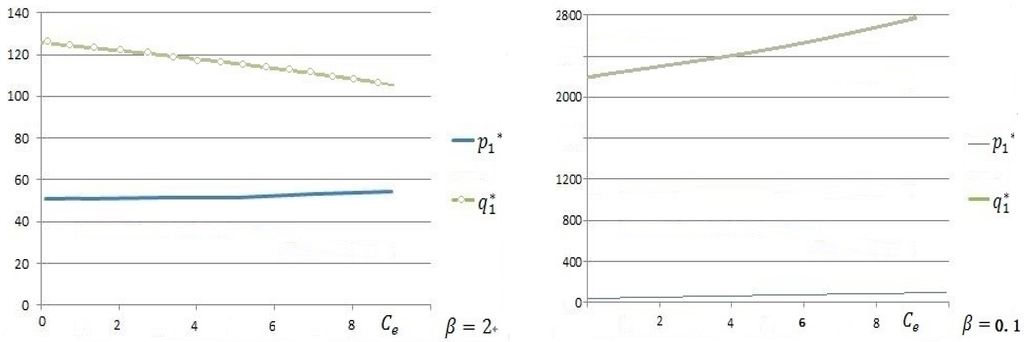
Figure 1. The effect of $C_e$ on ${p_1}^{*}/q_1^{*}$.

Figure 1. The effect of $C_e$ on ${p_1}^{*}/q_1^{*}$.

Figure 2 reveals that ${\lambda }^{*}$ changes with the carbon emissions trading price $C_e$. Such change is related to consumers’ sensitivity to carbon emissions. If $\gamma =0$, when $C_e\le 0.6$, ${\lambda }^{*}=0$ and mode 2 is the optimum transportation. When $C_e\ge 0.6$, ${\lambda }^{*}=1$, mode 1 is the optimum. If $\gamma =10$, ${\lambda }^{*}=1$, mode 1 is the first choice of the retailer at all times. This demonstrates that if consumers show high preference for low-carbon products, retailers will choose low-carbon transportation modes even though the government has not implemented a carbon cap-and-trade policy. Low-carbon awareness of consumers could drive the retailer to choose a low-carbon transportation mode. However, if consumers are less sensitive to carbon emissions, the government must control the carbon emissions trading price within an appropriate range through related policies and macroeconomic regulation. It is only in this way that retailers will choose low-carbon transportation modes. Additionally, viewed from the perspective of the retailer, transportation mode selection shall adapt to fluctuations in the carbon emissions trading price in order to gain the maximum profit.

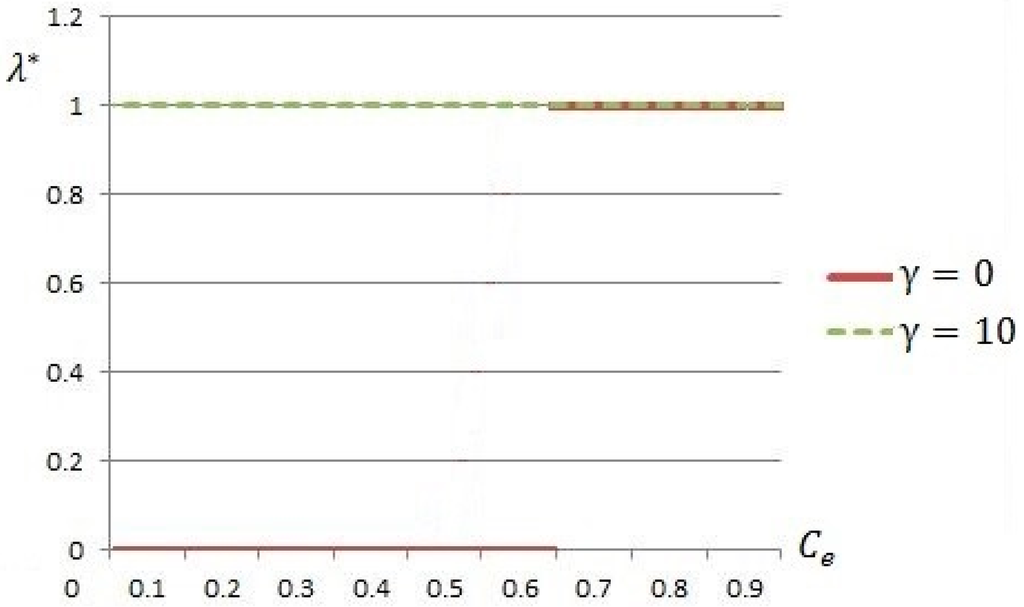
Figure 2. The effect of $C_e$ on ${\lambda }^{*}$.

Figure 2. The effect of $C_e$ on ${\lambda }^{*}$.

According to Figure 3 and Figure 4, the carbon emissions of the retailer will change with $C_e$. Different consumer sensitivity to carbon emissions will lead to different effects of carbon emissions trading prices on carbon emissions. Within the range of $0\le C_e\le 0.6$, the total carbon emissions of the retailer are low when consumers are highly sensitive to carbon emissions. This is because consumers’ sensitivity to carbon emissions forces the retailer to choose low-carbon transportation. Meanwhile, different consumer sensitivity to price will affect carbon emissions to a certain extent. It can be observed that within $0\le C_e\le 0.6$ and $C_e>0.6$ in Figure 3 as well as Figure 4, the higher carbon emissions trading price results in lower ($\beta =2$)/higher ($\beta =0.1$) carbon emissions.

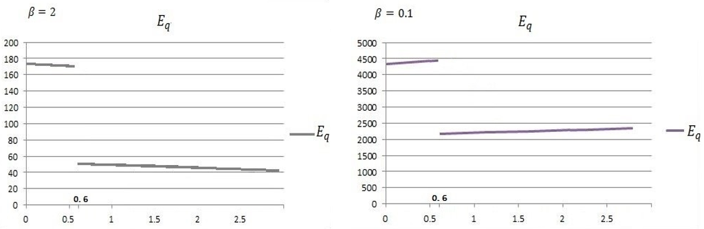
Figure 3. The effect of $C_e$ on $E_q$ $\left(\gamma =0\right)$.

Figure 3. The effect of $C_e$ on $E_q$ $\left(\gamma =0\right)$.

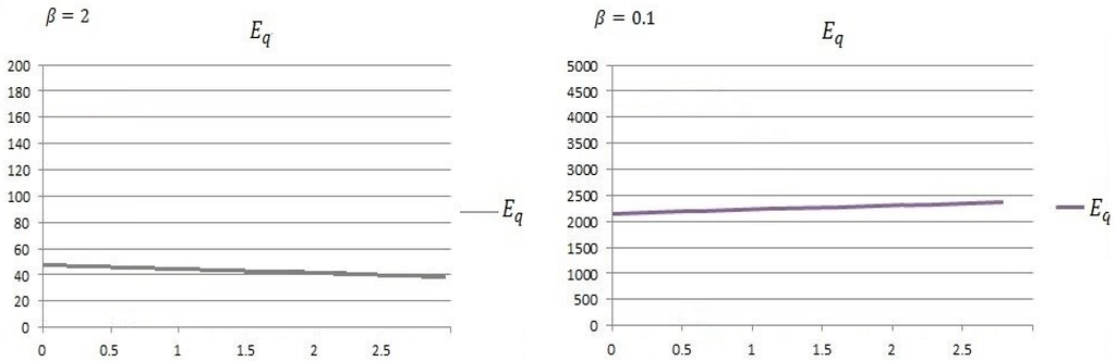
Figure 4. The effect of $C_e$ on $E_q$ $\left(\gamma =10\right)$.

Figure 4. The effect of $C_e$ on $E_q$ $\left(\gamma =10\right)$.

If other parameters are fixed, the decision-making of the retailer will vary in accordance with the change of transportation costs and transportation-induced carbon emissions:

It can be seen from Figure 5 that the optimum order quantity of the retailer will be influenced by both transportation costs and transportation-induced carbon emissions. When $\beta =2$, that is, consumers are greatly sensitive to price, the optimum order quantity is inversely proportional to transportation costs and transportation-induced carbon emissions. This means that the general transportation cost increases slightly, while market demand and order quantity reduce. When $\beta =0.1$, that is, consumers are insensitive to price but prefer low-carbon products, the order quantity is proportional to transportation costs and transportation-induced carbon emissions.

Figure 5. Variation of the optimum order quantity with transportation costs and transportation-induced carbon emissions.

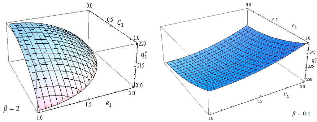
Figure 5. Variation of the optimum order quantity with transportation costs and transportation-induced carbon emissions.

Figure 6 illustrates that the retail price of a product is proportional to transportation costs and transportation-induced carbon emissions. When $\beta =2$, that is, the optimum retail price is far smaller than $\beta =0.1$, there will be certain capacity of the market as long as the price is controlled within a certain range, because consumers are very sensitive to price. When $\beta$ is small, the consumers are less sensitive to price, but highly sensitive to carbon emissions. Price is not the main priority of consumers. This is why there is great difference in the optimum retail price when $\beta$ is different.

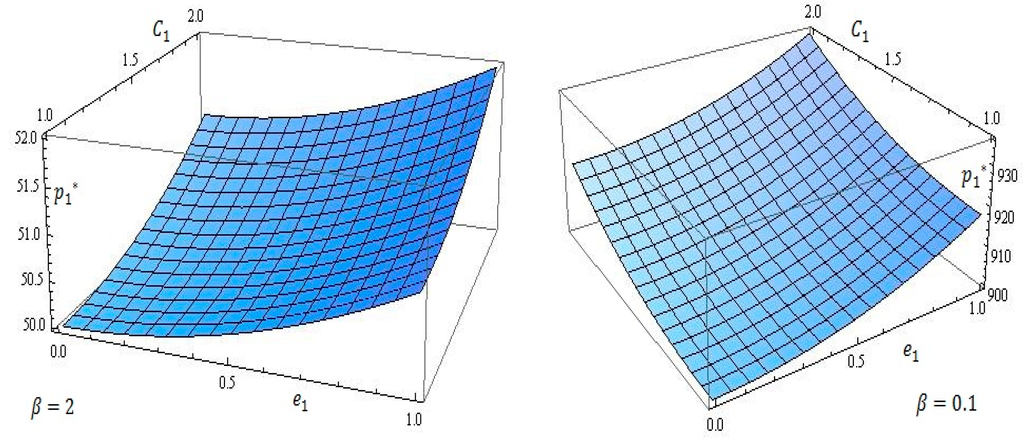
Figure 6. Variation of the optimal retail price with transportation costs and transportation-induced carbon emissions.

Figure 6. Variation of the optimal retail price with transportation costs and transportation-induced carbon emissions.

If other parameters are fixed, the decision-making of the retailer will change upon the fluctuation in consumer sensitivity to carbon emissions, which is shown in Figure 7 and Figure 8:

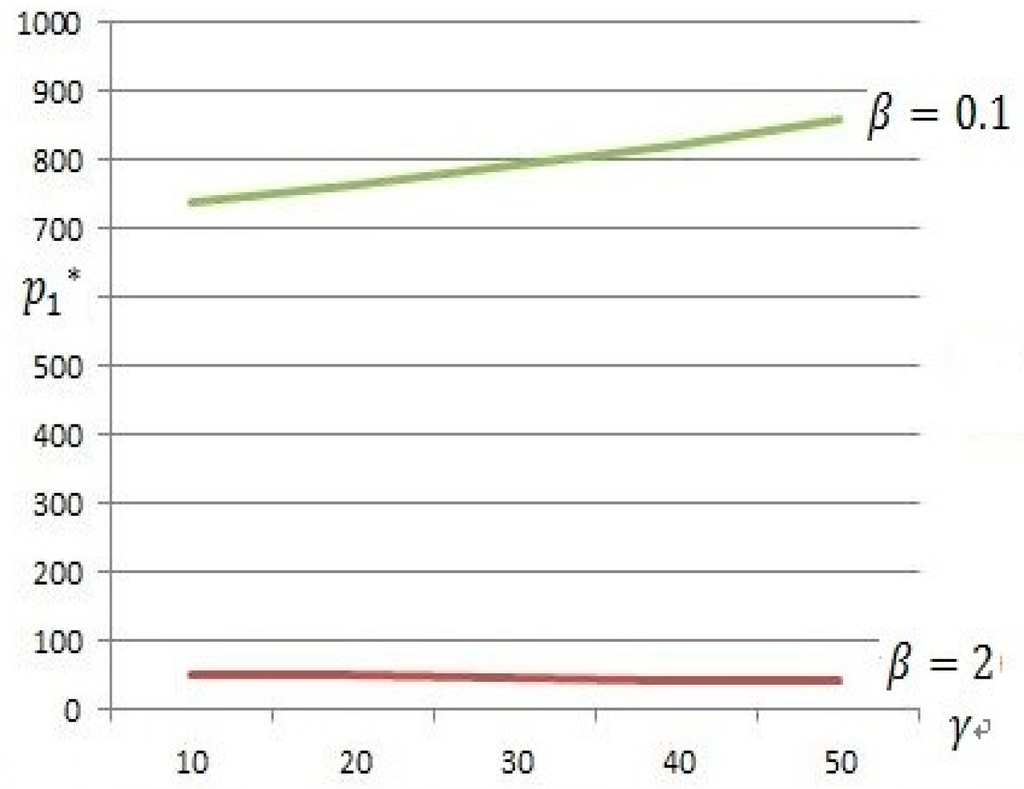
Figure 7. Variation of retail price with consumer sensitivity to carbon emissions.

Figure 7. Variation of retail price with consumer sensitivity to carbon emissions.

Figure 8. Variation of order quantity with consumer sensitivity to carbon emissions.

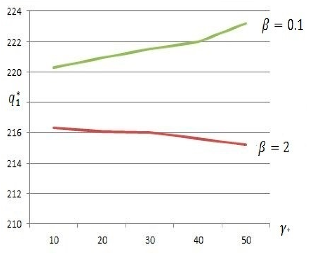
Figure 8. Variation of order quantity with consumer sensitivity to carbon emissions.

It can be deduced from Figure 7 and Figure 8 that when $\beta =2$, as consumers’ sensitivity to carbon emissions intensifies, the optimum retail price decreases slightly, but the optimum order quantity drops significantly. Since consumers are more sensitive to price than carbon emissions, the order quantity drops significantly although the retail price changes only slightly. When $\beta =0.1$, the optimum retail price and the optimum order quantity increase sharply as consumers’ sensitivity to carbon emissions increases.

7. Conclusions and Further Research

Based on uncertain market demand, this paper has investigated transportation mode selection, pricing and order quantity of retailers considering both consumers’ price-sensitive and carbon emission-sensitive demands under the influence of a carbon cap-and-trade policy. Firstly, the optimum transportation, pricing and ordering strategies for the retailer have been determined through modeling and analysis. Secondly, the effects of the initial emissions allowances and the carbon emissions trading price in the carbon cap-and-trade policy, as well as transportation costs and transportation-induced carbon emissions of different transportation modes, and consumer sensitivity to carbon emissions on decision-making and profit of the retailer have been discussed through a sensitivity analysis. The results of this paper have demonstrated that:

(1)

When consumers’ sensitivity to price is lower than the critical value ${\beta }_0$, the optimum retail price and the optimum order quantity are proportional to the transportation cost, the transportation-induced carbon emissions, the carbon emissions trading price, and the consumers’ sensitivity to carbon emissions.

(2)

When consumers’ sensitivity to price is higher than the critical value, the optimum order quantity of the retailer is inversely proportional to the transportation cost, the transportation-induced carbon emissions, the carbon emissions trading price and the consumers’ sensitivity to carbon emissions. The optimum retail price of the product and the retailer profit are inversely proportional to consumer sensitivity to carbon emissions.

(3)

The initial emission allowances are proportional to the expected profit of the retailer. Finally, these conclusions are further verified through a numerical analysis. Meanwhile, it was discovered that the carbon emissions trading price influences the carbon emissions trading volume of the retailer. When the carbon emissions trading price is high, the retailer will choose low-carbon transportation.

The contribution of this paper can be summarized as follows: Firstly, our article is one of few studies that have examined the effect of carbon cap and trade policy on a firm’s pricing, ordering and transportation mode selection considering consumer carbon-sensitive demand. Secondly, our research findings provide interesting managerial insights that will support retailers in making important operational and strategic decisions such as optimal pricing, optimal ordering quantity and transportation mode under a carbon cap and trade policy. Thirdly, our findings have indicated that it is wise for the government to develop effective carbon emissions reduction polices as part of their strategies to achieve sustainable development of the economy.

The research conclusions of this paper provide valuable insights in enterprise management. They not only address the economic benefits and environmental responsibilities of retailers, but also offer low-carbon retailers support in making important strategic and operational decisions. Future research will be conducted incorporating multiple research perspectives, multiple products and competition between retailers. The research findings of this paper can be expanded from the decision-making of a single retailer to the whole supply chain. Moreover, we can discuss different carbon emission policies and draw attention to carbon caps and taxes.

References

- Pan, S.; Ballot, E.; Fontane, F. The reduction of greenhouse gas emissions from freight transport by pooling supply chains. Int. J. Prod. Econ. 2013, 143, 86–94. [Google Scholar] [CrossRef]
- Cristea, A.; Hummels, D.; Puzzello, L.; Avetisyan, M. Trade and the greenhouse gas emissions from international freight transport. J. Environ. Econ. Manag. 2013, 65, 153–173. [Google Scholar] [CrossRef]
- Gaker, D.; Walker, J.L. Revealing the value of “green” and the small group with a big heart in transportation mode choice. Sustainability 2013, 5, 2913–2927. [Google Scholar] [CrossRef]
- Yildirim, M.B.; Mouzon, G. Single-machine sustainable production planning to minimize total energy consumption and total completion time using a multiple objective genetic algorithm. IEEE Trans. Eng. Manag. 2013, 59, 585–597. [Google Scholar] [CrossRef]
- Ouyang, B.; Li, Z.K.; Feng, Z.H. The current situation, problems and prospect of research on low-carbon transport planning. China Bus. Mark. 2014, 240, 13–20. [Google Scholar]
- Bansal, S.; Gangopadhyay, S. Tax/subsidy policies in the presence of environmental aware consumers. J. Environ. Econ. Manag. 2003, 45, 333–355. [Google Scholar] [CrossRef]
- Innes, R. A theory of consumer boycotts under symmetric information and imperfect competition. Econ. J. 2006, 116, 355–381. [Google Scholar] [CrossRef]
- Chen, J. Study on supply chain management in a low-carbon Era. J. Syst. Manag. 2012, 21, 721–728. [Google Scholar]
- Congress of the United States. Policy Options for Reducing CO2 Emissions: A CBO Study; Congressional Budget Office (CBO): Washington, DC, USA, 2008. [Google Scholar]
- Zhang, B.; Xu, L. Multi-item production planning with carbon cap and trade mechanism. Int. J. Prod. Econ. 2013, 144, 118–127. [Google Scholar] [CrossRef]
- Benjaafar, S.; Li, Y.; Daskin, M. Carbon footprint and the management of supply chains: Insights from simple models. IEEE Trans. Autom. Sci. Eng. 2013, 10, 99–116. [Google Scholar] [CrossRef]
- Song, J.; Leng, M. Analysis of the single-period problem under carbon emissions policies. In Handbook of Newsvendor Problems; Springer: Berlin, Germany, 2012; pp. 297–313. [Google Scholar]
- Zhao, D.Z.; Wang, C.G. A research on emission reduction decisions in supply chain with low-carbon policy considered. Ind. Eng. J. 2014, 17, 105–111. [Google Scholar]
- Diabat, A.; Abdallah, T.; Al-Refaie, A.; Svetinovic, D.; Govindan, K. Strategic closed-loop facility location problem with carbon market trading. IEEE Trans. Eng. Manag. 2013, 60, 398–408. [Google Scholar] [CrossRef]
- Du, S.; Ma, F.; Fu, Z.; Zhu, L.; Zhang, J. Game-theoretic analysis for an emission-dependent supply chain in a ‘cap-and-trade’ system. Ann. Oper. Res. 2015, 228, 135–149. [Google Scholar] [CrossRef]
- Wahab, M.I.M.; Mamun, S.M.H.; Ongkunaruk, P. EOQ models for a coordinated two-level international supply chain considering imperfect items and environmental impact. Int. J. Prod. Econ. 2011, 134, 151–158. [Google Scholar] [CrossRef]
- Yang, H.; Chung, C.Y.; Wong, K.P. Optimal fuel, power and load-based emissions trades for electric power supply chain equilibrium. IEEE Trans. Power Syst. 2012, 27, 1147–1157. [Google Scholar] [CrossRef]
- Purohit, A.K.; Choudhay, D.; Shankar, R. Inventory lot-sizing under dynamic stochastic demand with carbon emission constraints. Procedia Soc. Behav. Sci. Eng. 2015, 189, 193–197. [Google Scholar] [CrossRef]
- Purohit, A.K.; Shankar, R.; Dey, P.K.; Choudhary, D. Non-stationary stochastic inventory lot-sizing with emission and service level constraints in a carbon cap-and-trade system. J. Clean. Prod. 2015. [Google Scholar] [CrossRef]
- Conrad, K. Price competition and product differentiation when consumers care for the environment. Environ. Resour. Econ. 2005, 31, 1–19. [Google Scholar] [CrossRef]
- Liu, Z.L.; Anderson, T.D.; Cruz, J.M. Consumer environmental awareness and competition in two-stage supply chains. Eur. J. Oper. Res. 2012, 218, 602–613. [Google Scholar] [CrossRef]
- Nouira, I.; Frein, Y.; Hadj-Alouane, A.B. Optimization of manufacturing systems under environmental considerations for a greenness-dependent demand. Int. J. Prod. Econ. 2014, 150, 188–198. [Google Scholar] [CrossRef]
- Chang, T.S. Best routes selection in international intermodal networks. Comput. Oper. Res. 2013, 39, 111–114. [Google Scholar] [CrossRef]
- Liao, C.H.; Tseng, P.H.; Lu, C.S. Comparing carbon dioxide emissions of trucking and intermodal container transport in Taiwan. Transp. Res. D 2009, 14, 493–496. [Google Scholar] [CrossRef]
- Liao, C.H.; Lu, C.S.; Tseng, P.H. Carbon dioxide emissions and inland container transport in Taiwan. J. Transp. Geogr. 2011, 19, 722–728. [Google Scholar] [CrossRef]
- Goel, A. The value of in-transit visibility for supply chains with multiple modes of transport. Int. J. Logist. Res. Appl. 2010, 13, 475–492. [Google Scholar] [CrossRef]
- Janic, M. Assessing some social and environmental effects of transforming an airport into a real multimodal transport node. Transp. Res. D 2011, 16, 137–149. [Google Scholar] [CrossRef]
- McKinnon, A.C.; Woodburn, A. Logistical restructuring and road freight traffic growth: An empirical assessment. Transportation 1996, 23, 141–161. [Google Scholar] [CrossRef]
- Leal, I.C., Jr.; D’Agosto, M.A. Modal choice evaluation of transport alternatives for exporting bio-ethanol from Brazil. Transp. Res. D 2011, 16, 201–207. [Google Scholar] [CrossRef]
- Cholette, S.; Venkat, K. The energy and carbon intensity of wine distribution: A study of logistical options for delivering wine to consumers. J. Clean. Prod. 2009, 17, 1401–1413. [Google Scholar] [CrossRef]
- Hoen, K.M.R.; Tan, T.; Fransoo, J.C.; van Houtum, G.J. Switching transport modes to meet voluntary carbon emission targets. Transp. Sci. 2013, 48, 592–608. [Google Scholar] [CrossRef]
- Hoen, K.M.R.; Tan, T.; Fransoo, J.C.; van Houtum, G.J. Effect of carbon emission regulations on transport mode selection under stochastic demand. Flex. Serv. Manuf. J. 2014, 26, 170–195. [Google Scholar] [CrossRef]
- Chen, X.; Wang, X.J. Effects of carbon emission reduction policies on transportation mode selections with stochastic demand. Transp. Res. E 2015. [Google Scholar] [CrossRef]
- Wang, X.; Chan, H.K.; Li, D. A case study of integrated fuzzy methodology for green product development. Eur. J. Oper. Res. 2015, 241, 212–223. [Google Scholar] [CrossRef]
- Petruzi, N.C.; Dada, M. Pricing and the newsvendor problem: A review with extensions. Oper. Res. 1999, 47, 183–194. [Google Scholar] [CrossRef]
© 2016 by the authors; licensee MDPI, Basel, Switzerland. This article is an open access article distributed under the terms and conditions of the Creative Commons by Attribution (CC-BY) license (http://creativecommons.org/licenses/by/4.0/).