
Optimal Path for Controlling Sectoral CO2 Emissions Among China’s Regions: A Centralized DEA Approach

Abstract
:1. Introduction
2. Literature Review
3. Methodology
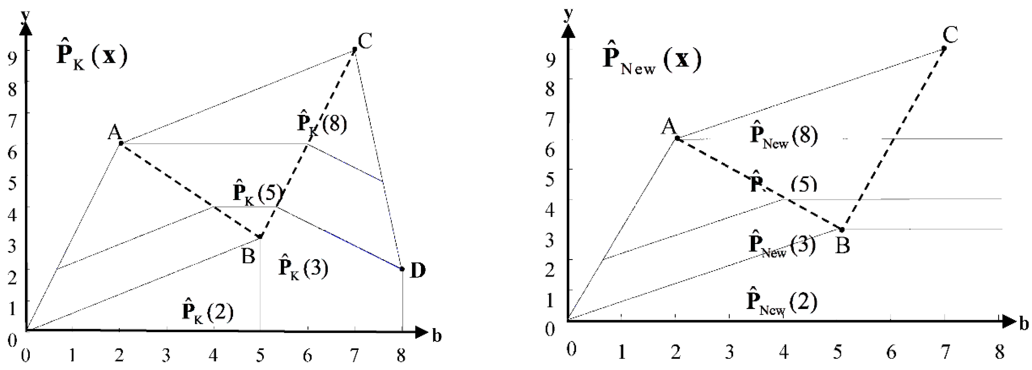
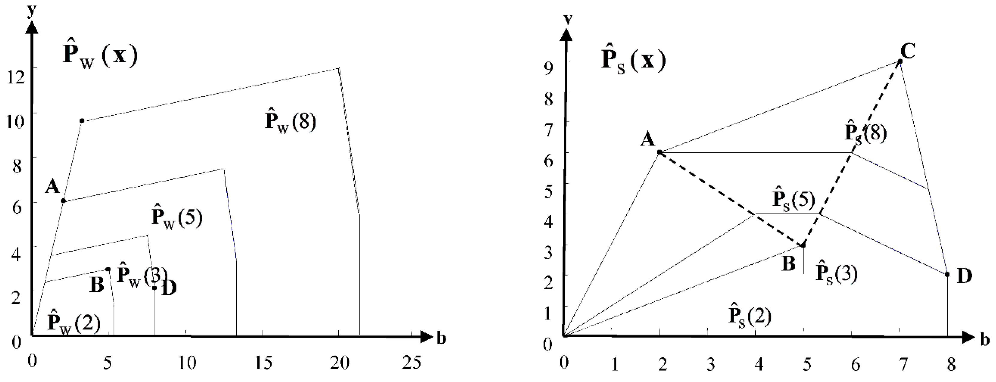
3.1. Environmental DEA Technology
- (1)
- If and , then (weak disposability for desirable and undesirable outputs).
- (2)
- If and , then (null-jointness of desirable and undesirable outputs).


| DMU | A | B | C | D |
|---|---|---|---|---|
| b | 2 | 5 | 7 | 8 |
| x | 5 | 2 | 8 | 3 |
| y | 6 | 3 | 9 | 2 |
3.2. Centralized Model for New Environmental DEA Technology
- (1)
- , can be defined as total control strategy, which implies that the total undesirable outputs permitted is equal to multiplied by the aggregate baseline undesirable outputs from all DMU.
- (2)
- , we define it as sectoral control strategy, which denotes the optimized sum of aggregated undesirable outputs produced by activities refer to environmental production technology s, which will be equal to times from observed aggregated undesirable outputs produced by activities.
4. Empirical Study
4.1. Data
| Index | Sector | Unit | Dimension | Quantity | Mean | Standard Deviation | Minimum | Maximum |
|---|---|---|---|---|---|---|---|---|
| Capital Stock (2000 constant price) | Agriculture | 100 million RMB | provincial sector | 29×17 | 379.46 | 417.68 | 25.61 | 2843.24 |
| Manufacturing | 100 million RMB | provincial sector | 29×17 | 6182.51 | 6558.73 | 274.76 | 48,577.60 | |
| Construction | 100 million RMB | provincial sector | 29×17 | 186.14 | 219.64 | 9.30 | 2134.61 | |
| Transportation | 100 million RMB | provincial sector | 29×17 | 1905.75 | 1687.42 | 61.25 | 9526.33 | |
| Service | 100 million RMB | provincial sector | 29×17 | 6370.96 | 7042.74 | 145.72 | 39,632.95 | |
| Labor Force | Agriculture | 10 thousand persons | provincial sector | 29×17 | 1099.34 | 853.02 | 37.09 | 3996.00 |
| Manufacturing | 10 thousand persons | provincial sector | 29×17 | 426.05 | 399.76 | 19.60 | 2283.46 | |
| Construction | 10 thousand persons | provincial sector | 29×17 | 146.53 | 141.98 | 9.80 | 715.10 | |
| Transportation | 10 thousand persons | provincial sector | 29×17 | 87.86 | 84.37 | 8.40 | 792.02 | |
| Service | 10 thousand persons | provincial sector | 29×17 | 594.30 | 396.37 | 40.70 | 1915.42 | |
| Energy (standard coal equivalent) | Agriculture | 10 thousand tons | provincial sector | 29×17 | 179.18 | 122.51 | 7.96 | 691.64 |
| Manufacturing | 10 thousand tons | provincial sector | 29×17 | 3702.02 | 3135.19 | 76.72 | 17,649.98 | |
| Construction | 10 thousand tons | provincial sector | 29×17 | 74.77 | 82.01 | 1.12 | 605.01 | |
| Transportation | 10 thousand tons | provincial sector | 29×17 | 493.44 | 477.83 | 13.73 | 2716.30 | |
| Service | 10 thousand tons | provincial sector | 29×17 | 318.02 | 297.73 | 3.13 | 1969.78 | |
| Value Added (2000 constant price) | Agriculture | 100 million RMB | provincial sector | 29×17 | 600.36 | 450.00 | 33.51 | 2065.31 |
| Manufacturing | 100 million RMB | provincial sector | 29×17 | 2567.06 | 3115.48 | 42.99 | 19,950.01 | |
| Construction | 100 million RMB | provincial sector | 29×17 | 343.27 | 299.55 | 14.45 | 1760.92 | |
| Transportation | 100 million RMB | provincial sector | 29×17 | 399.12 | 409.84 | 8.44 | 2916.87 | |
| Service | 100 million RMB | provincial sector | 29×17 | 1671.10 | 1735.37 | 50.31 | 10,590.03 | |
| CO2 | Agriculture | 10 thousand tons | provincial sector | 29×17 | 565.88 | 374.80 | 22.43 | 1948.69 |
| Manufacturing | 10 thousand tons | provincial sector | 29×17 | 12,408.36 | 10,493.94 | 265.52 | 58,033.89 | |
| Construction | 10 thousand tons | provincial sector | 29×17 | 220.54 | 220.70 | 8.03 | 1598.10 | |
| Transportation | 10 thousand tons | provincial sector | 29×17 | 1148.49 | 1064.41 | 33.30 | 6123.26 | |
| Service | 10 thousand tons | provincial sector | 29×17 | 1082.89 | 1004.35 | 17.84 | 6034.86 |
| Area | Economic Region | Provinces |
|---|---|---|
| East | Northern Coastal | Beijing, Tianjin, Hebei, Shandong |
| Eastern Coastal | Shanghai, Jiangsu, Zhejiang | |
| Southern Coastal | Fujian, Guangdong, Hainan | |
| Central | Middle Yellow River | Shanxi, Inner Mongolia, Henan, Shaanxi |
| Middle Yangtze River | Anhui, Jiangxi, Hubei, Hunan | |
| West | Southwest | Guangxi, Chongqing+Sichuan, Guizhou, Yunan |
| Northwest | Gansu, Qinghai, Ningxia, Xinjiang | |
| Northeast | Northeast | Liaoning, Jilin, Heilongjiang |
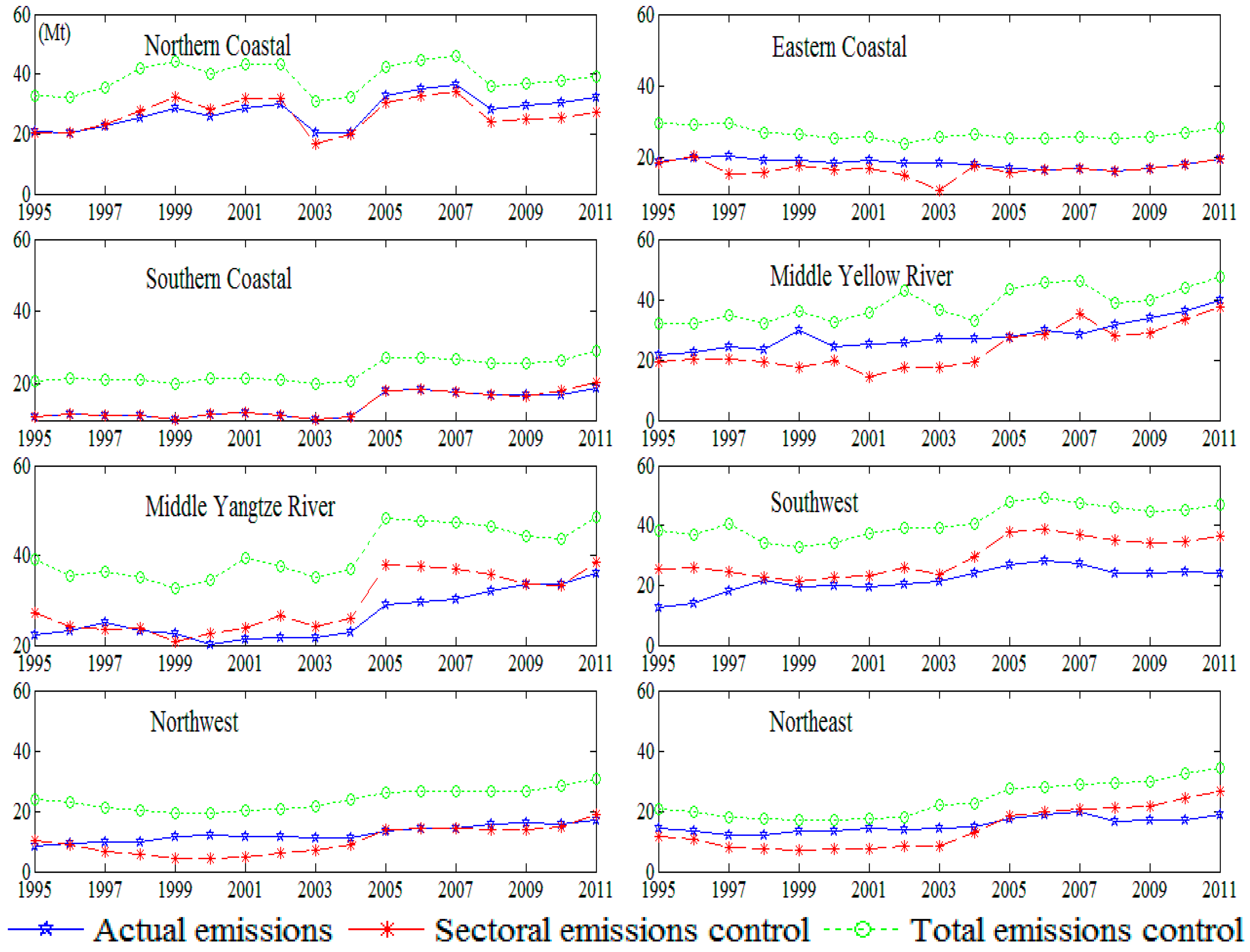
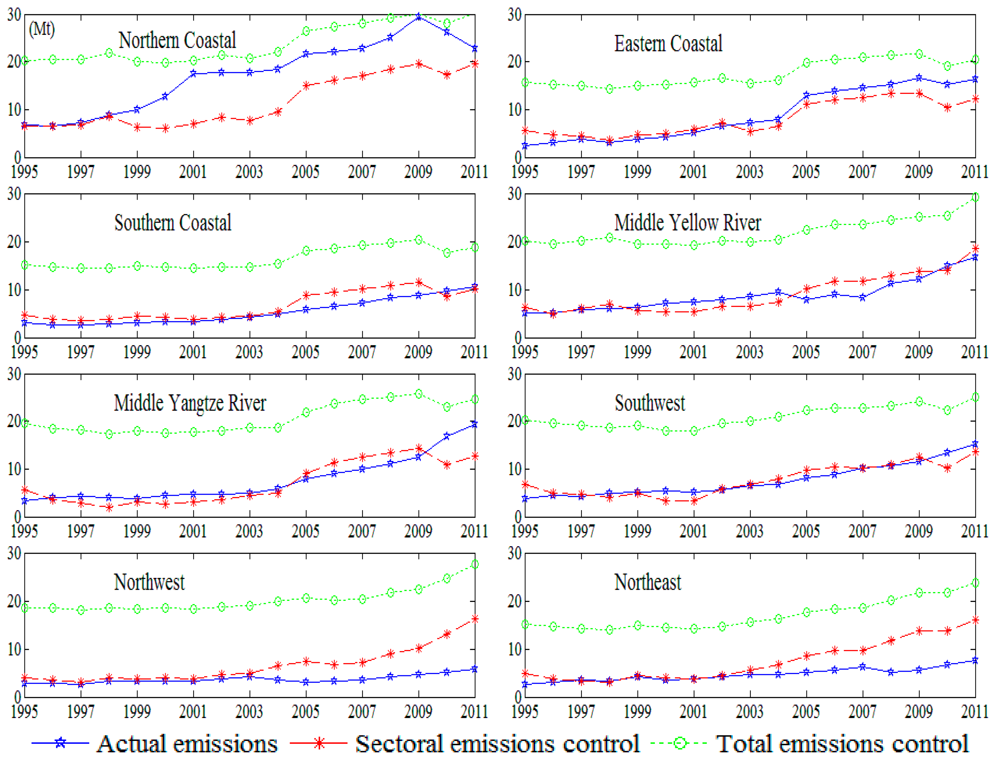
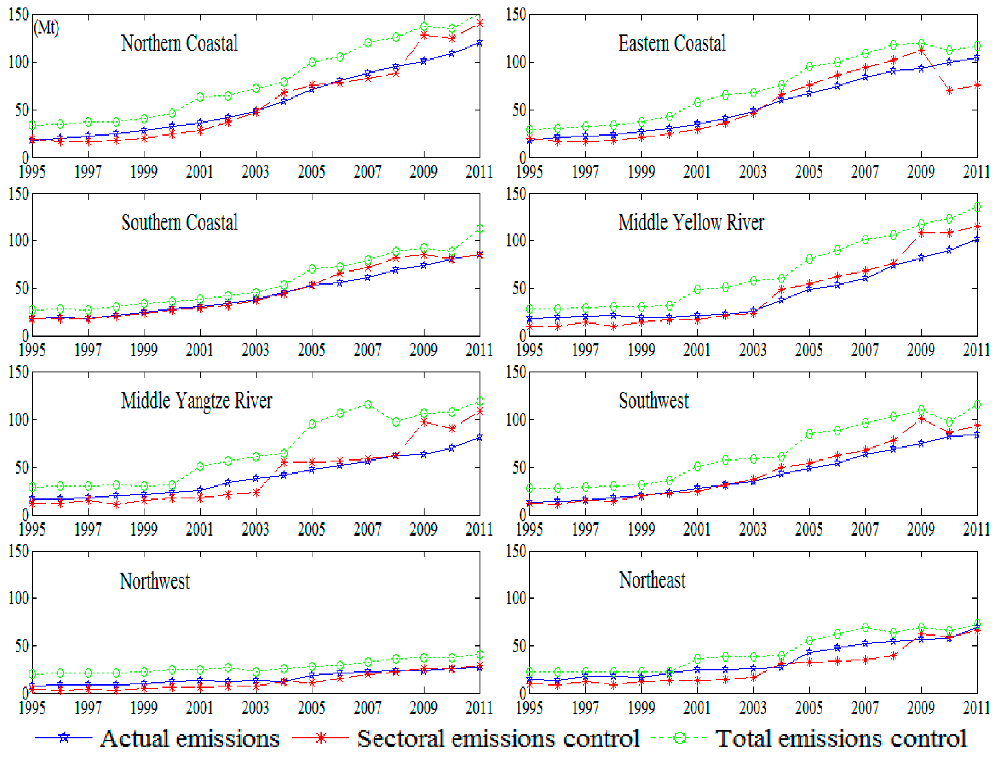
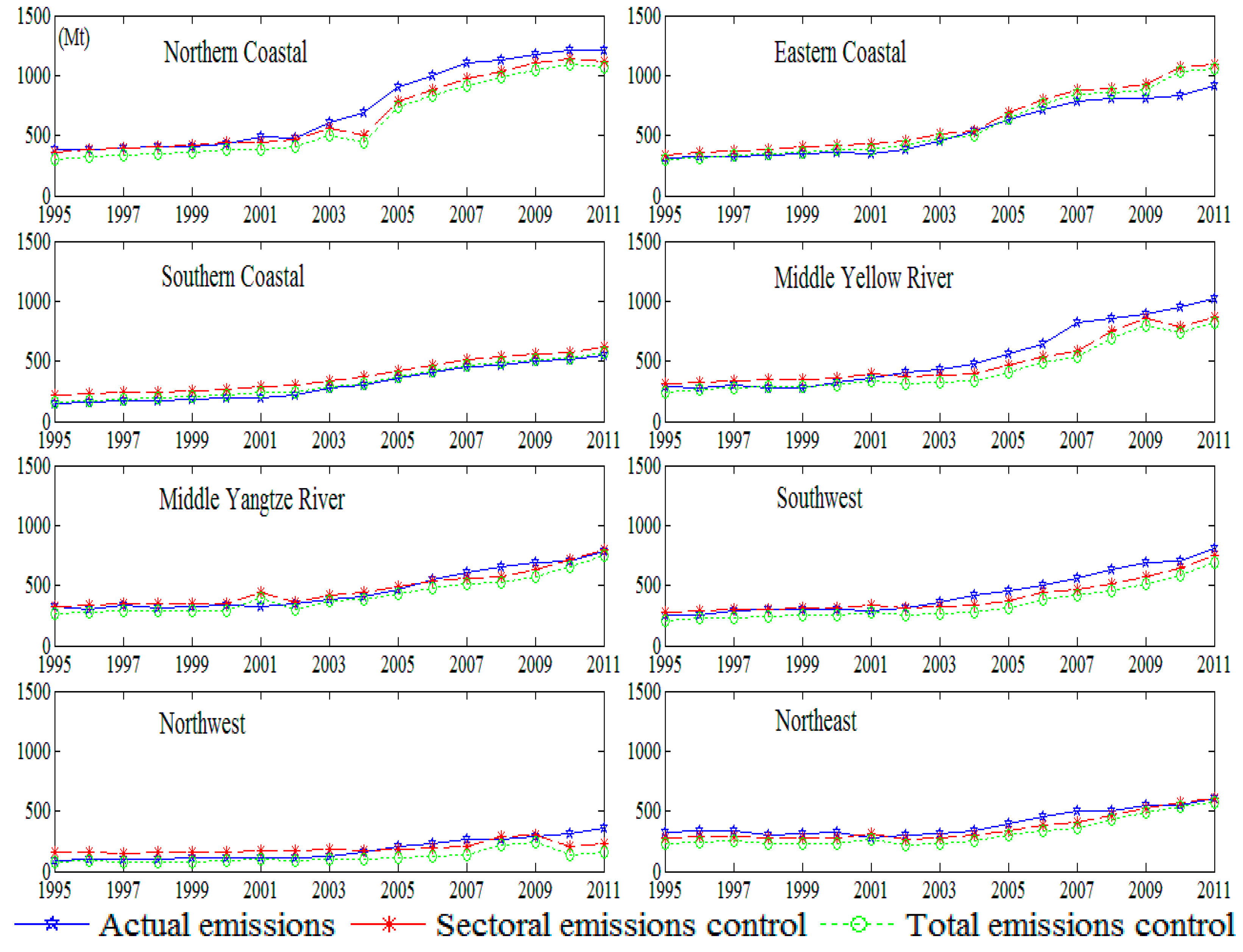
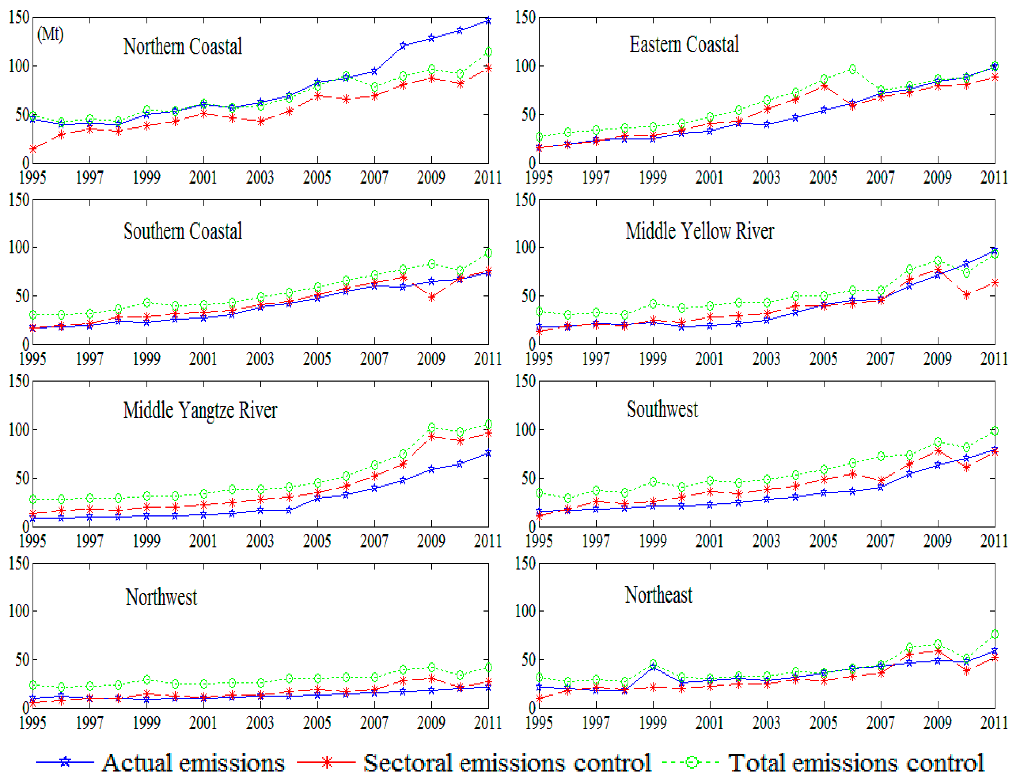
4.2. Main Results


| Sector | Deviation Under Sectoral Emissions Control | Deviation Under Total Emissions Control | ||
|---|---|---|---|---|
| Degree | Quantity (Unit: 10 Thousand Tons) | Degree | Quantity (Unit: 10 Thousand Tons) | |
| Agriculture | 0.635 | 0 | 0.091 | 173655 |
| Manufacturing | 0.128 | 0 | 0.072 | -784174 |
| Construction | 1.984 | 0 | 0.141 | 173426 |
| Transportation | 0.539 | 0 | 0.183 | 259380 |
| Service | 0.439 | 0 | 0.081 | 177712 |
| Area | Deviation Under Sectoral Emissions Control | Deviation Under Total Emissions control | ||
|---|---|---|---|---|
| Degree | Quantity (Unit: 10 Thousand Tons) | Degree | Quantity (Unit: 10 Thousand Tons) | |
| East | 0.951 | 117,672 | 0.908 | 123,870.9 |
| Central | 1.146 | −47,519.2 | 1.123 | −28,893.7 |
| West | 1.758 | 1932.418 | 1.939 | −28,708.4 |
| Northeast | 1.794 | −72,085.3 | 1.905 | −66,268.8 |
| Year (1995–2011) | Agriculture | Manufacturing | Construction | Transportation | Service | ||||||||||
|---|---|---|---|---|---|---|---|---|---|---|---|---|---|---|---|
| DDF | SEC | TEC | DDF | SEC | TEC | DDF | SEC | TEC | DDF | SEC | TEC | DDF | SEC | TEC | |
| Average | −0.504 | −0.050 | 0 | −0.090 | 0 | 0 | −1.471 | 0 | 0 | −0.152 | −0.109 | 0 | −0.921 | −0.057 | 0 |
5. Conclusions
Acknowledgments
Author Contributions
Conflicts of Interest
References
- Stern, N. The Economics of Climate Change: The Stern Review; Cambridge University Press: Cambrige, UK, 2007. [Google Scholar]
- Liu, Z. China’s Carbon Emissions Report 2015; Harvard Kennedy School: Cambridge, UK, 2015. [Google Scholar]
- Färe, R.; Grosskopf, S.; Kokkelenberg, E.C. Measuring plant capacity, utilization and technical change: A nonparametric approach. Int. Econ. Rev. 1989, 41, 655–666. [Google Scholar] [CrossRef]
- Färe, R.; Grosskopf, S.; Margaritis, D.; Weber, W. Technological change and timing reductions in greenhouse gas emissions. J. Product. Anal. 2012, 37, 205–216. [Google Scholar] [CrossRef]
- Färe, R.; Grosskopf, S.; Pasurka, C.A., Jr. Potential gains from trading bad outputs: The case of US electric power plants. Resour. Energy Econ. 2014, 36, 99–112. [Google Scholar] [CrossRef]
- Zhou, P.; Sun, Z.R.; Zhou, D.Q. Optimal path for controlling CO2 emissions in China: A perspective of efficiency analysis. Energy. Econ. 2014, 45, 99–110. [Google Scholar] [CrossRef]
- Aparicio, J.; Pastor, J.T.; Zofio, J.L. On the inconsistency of the Malmquist–Luenberger index. Eur. J. Oper. Res. 2013, 229, 738–742. [Google Scholar] [CrossRef]
- Färe, R.; Grosskopf, S.; Pasurka, C. Technical change and pollution abatement costs. Eur. J. Oper. Res. 2016, 248, 715–724. [Google Scholar] [CrossRef]
- Charnes, A.; Cooper, W.W.; Rhodes, E. Measuring the efficiency of decision making units. Eur. J. Oper. Res. 1978, 2, 429–444. [Google Scholar] [CrossRef]
- Kuosmanen, T.; Cherchye, L.; Sipiläinen, T. The law of one price in data envelopment analysis: Restricting weight flexibility across firms. Eur. J. Oper. Res. 2006, 170, 735–757. [Google Scholar] [CrossRef]
- Dantzig, G.B. Programming of interdependent activities: II mathematical model. Econometrica 1949, 17, 200–211. [Google Scholar] [CrossRef]
- Debreu, G. The coefficient of resource utilization. Econometrica 1951, 3, 273–292. [Google Scholar] [CrossRef]
- Koopmans, T.C. Analysis of production as an efficient combination of activities. Act. Anal. Prod. All. 1951, 13, 33–37. [Google Scholar]
- Koopmans, T.C. Efficient allocation of resources. Econometrica 1951, 19, 455–465. [Google Scholar] [CrossRef]
- Koopmans, T.C. Three Essays on the State of Economic Science; McGraw-Hill: New York, NY, USA, 1957. [Google Scholar]
- Afriat, S.N. Efficiency estimation of production functions. Int. Econ. Rev. 1972, 13, 568–598. [Google Scholar] [CrossRef]
- Banker, R.D.; Maindiratta, A. Nonparametric analysis of technical and allocative efficiencies in production. Econometrica 1988, 56, 1315–1332. [Google Scholar] [CrossRef]
- Färe, R.; Grosskopf, S. Nonparametric tests of regularity, Farrell efficiency, and goodness-of-fit. J. Econom. 1995, 69, 415–425. [Google Scholar] [CrossRef]
- Hanoch, G.; Rothschild, M. Testing the assumptions of production theory: A nonparametric approach. J. Polit. Econ. 1972, 80, 256–275. [Google Scholar] [CrossRef]
- Varian, H.R. The nonparametric approach to production analysis. Econometrica 1984, 52, 579–598. [Google Scholar] [CrossRef]
- Golany, B.; Tamir, E. Evaluating efficiency-effectiveness-equality trade-offs: A data envelopment analysis approach. Manag. Sci. 1995, 41, 1172–1184. [Google Scholar] [CrossRef]
- Lozano, S.; Villa, G. Centralised target setting for regional recycling operations using DEA. Omega 2004, 32, 101–110. [Google Scholar] [CrossRef]
- Li, S.K.; Ng, Y.C. Measuring the productive efficiency of a group of firms. Int. Adv. Econ. Res. 1995, 1, 377–390. [Google Scholar] [CrossRef]
- Asmild, M.; Paradi, J.C.; Pastor, J.T. Centralized resource allocation BCC models. Omega 2009, 37, 40–49. [Google Scholar] [CrossRef]
- Mar-Molinero, C.; Prior, D.; Segovia, M.-M.; Portillo, F. On centralized resource utilization and its reallocation by using DEA. Ann. Oper. Res. 2014, 221, 273–283. [Google Scholar] [CrossRef]
- Fang, L. A generalized DEA model for centralized resource allocation. Eur. J. Oper. Res. 2013, 228, 405–412. [Google Scholar] [CrossRef]
- Korhonen, P.; Syrjänen, M. Resource allocation based on efficiency analysis. Manag. Sci. 2004, 50, 1134–1144. [Google Scholar] [CrossRef]
- Hadi-Vencheh, A.; Foroughi, A.A.; Soleimani-damaneh, M. A DEA model for resource allocation. Econ. Model. 2008, 25, 983–993. [Google Scholar] [CrossRef]
- Amirteimoori, A.; Tabar, M.M. Resource allocation and target setting in data envelopment analysis. Expert. Syst. Appl. 2010, 37, 3036–3039. [Google Scholar] [CrossRef]
- Athanassopoulos, A.D. Goal programming & data envelopment analysis (GoDEA) for target-based multi-level planning: Allocating central grants to the Greek local authorities. Eur. J. Oper. Res. 1995, 87, 535–550. [Google Scholar]
- Gomes, E.G. Modelling undesirable outputs with zero sum gains data envelopment analysis models. J. Oper. Res. Soc. 2007, 59, 616–623. [Google Scholar] [CrossRef]
- Serro, A. Reallocating Agricultural Greenhouse Gas Emission in EU 15 Countries. In Proceeding of the Agricultural & Applied Economics Association 2010 AAEA, CAES, & WAEA Joint Annual Meeting, Denver, CO, USA, 25–27 July 2010.
- Wang, K.; Zhang, X.; Wei, Y.-M.; Yu, S. Regional allocation of CO2 emissions allowance over provinces in China by 2020. Energy Policy 2012, 54, 214–229. [Google Scholar] [CrossRef]
- Pang, R.-Z.; Deng, Z.-Q.; Chiu, Y.-H. Pareto improvement through a reallocation of carbon emission quotas. Renew. Sustain. Energy Rev. 2015, 50, 419–430. [Google Scholar] [CrossRef]
- Chiu, Y.-H.; Lin, J.-C.; Su, W.-N.; Liu, J.-K. An efficiency evaluation of the EU’s allocation of carbon emission allowances. Energy Sour. Part B Econ. Plan. Policy 2015, 10, 192–200. [Google Scholar] [CrossRef]
- Lozano, S.; Villa, G.; Brännlund, R. Centralised reallocation of emission permits using DEA. Eur. J. Oper. Res. 2009, 193, 752–760. [Google Scholar] [CrossRef]
- Wu, H.; Du, S.; Liang, L.; Zhou, Y. A DEA-based approach for fair reduction and reallocation of emission permits. Math. Comput. Model. 2013, 58, 1095–1101. [Google Scholar] [CrossRef]
- Singh, S.; Majumdar, S.S. Efficiency improvement strategy under constant sum of inputs. J. Math. Model. Algorithms Oper. Res. 2014, 13, 579–596. [Google Scholar] [CrossRef]
- Sun, J.; Wu, J.; Liang, L.; Zhong, R.Y.; Huang, G.Q. Allocation of emission permits using DEA: Centralised and individual points of view. Int. J. Prod. Res. 2014, 52, 419–435. [Google Scholar] [CrossRef]
- Homayounfar, M.; Amirteimoori, A.; Toloie-Eshlaghy, A. Production planning considering undesirable outputs-A DEA based approach. Int. J. Appl.Oper.Res. 2014, 4, 1–11. [Google Scholar]
- Feng, C.; Chu, F.; Ding, J.; Bi, G.; Liang, L. Carbon emissions abatement (CEA) allocation and compensation schemes based on DEA. Omega 2015, 53, 78–89. [Google Scholar] [CrossRef]
- Zhu, J. Data envelopment analysis with preference structure. J. Oper. Res. Soc. 1996, 47, 136–150. [Google Scholar] [CrossRef]
- Halme, M.; Joro, T.; Korhonen, P.; Salo, S.; Wallenius, J. A value efficiency approach to incorporating preference information in data envelopment analysis. Manag. Sci. 1999, 45, 103–115. [Google Scholar] [CrossRef]
- Zhou, P.; Fan, L. An extension to data envelopment analysis with preference structure for estimating overall inefficiency. Appl. Math. Comput. 2010, 216, 812–818. [Google Scholar] [CrossRef]
- Allen, R.; Athanassopoulos, A.; Dyson, R.G.; Thanassoulis, E. Weights restrictions and value judgements in data envelopment analysis: Evolution, development and future directions. Ann. Oper. Res. 1997, 73, 13–34. [Google Scholar] [CrossRef]
- Roll, Y.; Cook, W.D.; Golany, B. Controlling factor weights in data envelopment analysis. IIE Trans. 1991, 23, 2–9. [Google Scholar] [CrossRef]
- Podinovski, V. Production trade-offs and weight restrictions in data envelopment analysis. J. Oper. Res. Soc. 2004, 55, 1311–1322. [Google Scholar] [CrossRef]
- Førsund, F.R. Weight restrictions in DEA: Misplaced emphasis? J. Prod. Anal. 2013, 40, 271–283. [Google Scholar] [CrossRef]
- Färe, R.; Grosskopf, S.; Noh, D.-W.; Weber, W. Characteristics of a polluting technology: Theory and practice. J. Econom. 2005, 126, 469–492. [Google Scholar] [CrossRef]
- Zhou, P.; Ang, B.W.; Poh, K.L. Measuring environmental performance under different environmental DEA technologies. Energy Econ. 2008, 30, 1–14. [Google Scholar] [CrossRef]
- Färe, R.; Grosskopf, S. Nonparametric productivity analysis with undesirable outputs: Comment. Am. J. Agric. Econ. 2003, 85, 1070–1074. [Google Scholar] [CrossRef]
- Kuosmanen, T. Weak disposability in nonparametric production analysis with undesirable outputs. Am. J. Agric. Econ. 2005, 87, 1077–1082. [Google Scholar] [CrossRef]
- Kuosmanen, T.; Podinovski, V. Weak disposability in nonparametric production analysis: Reply to Färe and Grosskopf. Am. J. Agric. Econ. 2009, 91, 539–545. [Google Scholar] [CrossRef]
- Kuosmanen, T.; Kazemi Matin, R. Duality of weakly disposable technology. Omega 2011, 39, 504–512. [Google Scholar] [CrossRef]
- Leleu, H. Shadow pricing of undesirable outputs in nonparametric analysis. Eur. J. Oper. Res. 2013, 231, 474–480. [Google Scholar] [CrossRef]
- United Nations Framework Convention on Climate Change (UNFCCC). Kyoto Protocol to the United Nations Framework Convention on Climate Change; Kyoto Protocol: Kyoto, Japan, 1997. [Google Scholar]
- International Energy Agency (IEA). CO2 emissions from fuel combustion (2012 Edition); OECD Publishing: Paris, France, 2012. [Google Scholar]
- Färe, R.; Grosskopf, S.; Pasurka, C.A., Jr. Accounting for air pollution emissions in measures of state manufacturing productivity growth. J. Reg. Sci. 2001, 41, 381–409. [Google Scholar] [CrossRef]
- Zhang, J. Estimation of China’s provincial capital stock (1952–2004) with applications. J. Chin. Econ. Bus. Stud. 2008, 6, 177–196. [Google Scholar] [CrossRef]
- Guo, K.S. The driving factors to value added growth and the characteristics of changing for three industries. Jingji Yanjiu (Econ.Res. J.) 1992, 27, 51–61. (In Chinese) [Google Scholar]
- Gan, C.; Zheng, R. An empirical study on change of industrial structure and productivity growth since the reform and opening-up—A test for the structure-bonus hypotheses from 1978 to 2007 in China. Zhongguo Gongye Jingji (China Ind.Econ.) 2009, 251, 55–65. (In Chinese) [Google Scholar]
- Lv, T.; Zhou, S. Upgrading of an industrial structure and transformation of economic growth pattern in China. Guanli Shijie (Manag. World) 1999, 1999, 113–125. (In Chinese) [Google Scholar]
- National Bureau of Statistics of China. Statistical Yearbook of China’s Fixed Asset Investment 1982–1986, 1997–1999, and 2003–2012; China Planning Press: Beijing, China, 2012.
- National Bureau of Statistics of China. China Statistical Yearbook 1987-1996 and 2000–2002; China Statistics Press: Beijing, China, 2002.
- National Bureau of Statistics of China. China Labor Statistical Yearbook 1996–2012; China Statistics Press: Beijing, China, 2012.
- National Bureau of Statistics of China. China Statistical Yearbook 1996–2012; China Statistics Press: Beijing, China, 2012.
- National Bureau of Statistics of China. China Energy Statistical Yearbook 1996–2012; China Statistics Press: Beijing, China, 2012.
- Chung, Y.H.; Färe, R.; Grosskopf, S. Productivity and undesirable outputs: A directional distance function approach. J. Environ. Manag. 1997, 51, 229–240. [Google Scholar] [CrossRef]
© 2015 by the authors; licensee MDPI, Basel, Switzerland. This article is an open access article distributed under the terms and conditions of the Creative Commons by Attribution (CC-BY) license (http://creativecommons.org/licenses/by/4.0/).
Share and Cite
Sun, Z.; Luo, R.; Zhou, D. Optimal Path for Controlling Sectoral CO2 Emissions Among China’s Regions: A Centralized DEA Approach. Sustainability 2016, 8, 28. https://doi.org/10.3390/su8010028
Sun Z, Luo R, Zhou D. Optimal Path for Controlling Sectoral CO2 Emissions Among China’s Regions: A Centralized DEA Approach. Sustainability. 2016; 8(1):28. https://doi.org/10.3390/su8010028
Chicago/Turabian StyleSun, Zuoren, Rundong Luo, and Dequn Zhou. 2016. "Optimal Path for Controlling Sectoral CO2 Emissions Among China’s Regions: A Centralized DEA Approach" Sustainability 8, no. 1: 28. https://doi.org/10.3390/su8010028
APA StyleSun, Z., Luo, R., & Zhou, D. (2016). Optimal Path for Controlling Sectoral CO2 Emissions Among China’s Regions: A Centralized DEA Approach. Sustainability, 8(1), 28. https://doi.org/10.3390/su8010028